DESY 01–171
KANAZAWA 01-15
On the dynamics of color magnetic monopoles in full QCD

Abstract

We present first results on the dynamics of monopoles in full QCD with $N_{f}=2$ flavors of dynamical quarks. Among the quantities being studied are the monopole density and the monopole screening length, the static potential as well as the profile of the color electric flux tube. Furthermore, we derive the low-energy effective monopole action.

1 INTRODUCTION

In the dual superconductor picture of confinement the crucial degrees of freedom are the color magnetic monopoles revealed after abelian projection. In the maximally abelian gauge [1] one finds that the string tension is almost entirely due to monopole currents [2, 3], and that the low-energy effective monopole action reproduces the string tension and the low-lying glueball masses quite well [4]. Furthermore, the monopole currents show non-trivial correlations with gauge invariant excitations of the vacuum, such as the action and topological charge density [5, 6, 7]. The analysis of the monopole degrees of freedom may thus provide important information about the confinement mechanism. Past studies have mainly been restricted to the quenched approximation. It will be interesting now to see how the vacuum reacts to the presence of dynamical color electric charges.

Our studies will be done on $N_{f}=2$ dynamical gauge field configurations generated by the QCDSF and UKQCD collaborations using non-perturbatively $O(a)$ improved Wilson fermions [8]:

$$S_{F}=S^{(0)}_{F}-\frac{\rm i}{2}\kappa\,g\,c_{SW}a^{5}\sum_{x}\bar{\psi}(x)\sigma_{\mu\nu}F_{\mu\nu}\psi(x),$$

where $S^{(0)}_{F}$ is the original Wilson action.

The link variables $U(s,\mu)$ are brought into the maximally abelian gauge by maximizing the quantity [9]

$$R=\sum_{s,\mu}\,\sum_{i=1}^{3}|\widetilde{U}_{ii}(s,\mu)|^{2}$$ (1)

with respect to gauge transformations $g$:

$$\widetilde{U}(s,\mu)=g(s)U(s,\mu)g(s+\hat{\mu})^{-1},$$ (2)

using an $SU(3)$ update of the simulated annealing algorithm first introduced in [10] for $SU(2)$. The abelian link variables are defined by

$$u_{i}(s,\mu)\equiv e^{i\theta_{i}(s,\mu)}$$ (3)

with

$$\theta_{i}(s,\mu) = \arg\widetilde{U}_{ii}(s,\mu)$$ (4)

$$- \frac{1}{3}\sum_{j=1}^{3}\arg\widetilde{U}_{jj}(s,\mu)|_{{\rm mod}\,2\pi}.$$

2 MONOPOLE DENSITY

The first quantity we looked at is the monopole density. This is defined by

$$\rho=\frac{1}{12V}\sum_{s,\mu}\sum_{i=1}^{3}|k_{i}(s,\mu)|$$ (5)

where $k_{i}(s,\mu)$ are the monopole currents, which are obtained from the angles $\theta_{i}(s,\mu)$ [11], and $V$ is the lattice volume. The currents are subjected to the constraint $\sum_{i}k_{i}(s,\mu)=0$.

Figure 1: The monopole density for all clusters $(\times)$ and for large clusters $(\square)$.

The monopole currents fall into clusters of different lengths: large clusters are responsible for quark confinement, while short clusters are mainly due to ultraviolet fluctuations and have no effect on the confining forces [12]. As large clusters we count the largest cluster of the system and all clusters that wind around the lattice at least once. It was shown [13] (in pure $SU(2)$ gauge theory) that the density of monopoles belonging to the large clusters is finite in the continuum limit.

In Fig. 1 we show the monopole density for all clusters, and separately for the large clusters, as a function of $(m_{\pi}/m_{\rho})^{2}$. Also shown is the quenched result ($m_{\pi}/m_{\rho}=1$). The quenched data set, $\beta=6.0$, was chosen to match the lattice spacing of the dynamical configurations, $a\approx 0.1$ fm. The lattice volume varies between $16^{3}32$ and $24^{3}48$. We see that the monopole density is strongly affected by the presence of dynamical quarks. On the dynamical configurations the density is twice as large as on the quenched configurations with increasing tendency towards smaller quark masses.

3 STATIC POTENTIAL

Figure 2: The static potential $(\times)$ and the abelian static potential $(\square)$, with the self-energy subtracted. The upper figure is for $\beta=5.29,\kappa=0.135$, the lower figure for $\beta=6.0$ in the quenched theory.

The next quantity we have looked at is the static potential $V(r)$. This is computed from smeared Wilson loops. We parameterize the potential by

$$V(r)=V_{0}-\frac{e}{r}+\sigma\,r.$$ (6)

We also have looked at the abelian potential built from abelian link variables (3). This defines an abelian string tension $\sigma^{\rm ab}$. In Fig. 2 we show $V(r)$ and its abelian counterpart, and compare it with the quenched result. A fit gives $\sigma^{\rm ab}/\sigma=0.94(8)$ for the dynamical configuration shown and $\sigma^{\rm ab}/\sigma=1.03(15)$ for the quenched case.

Figure 3: The abelian static potential $(\times)$ divided into monopole $(\square)$ and photon $($$\circ$$)$ contributions. The upper figure is for $\beta=5.29,\kappa=0.135$, the lower figure for $\beta=6.0$ in the quenched theory.

It is instructive to separate the abelian gauge potential into a monopole and ‘photon’ part, $\theta(s,\mu)=\theta^{\rm mon}(s,\mu)+\theta^{\rm ph}(s,\mu)$ where

$$\theta^{\rm mon}(s,\mu)=-2\pi\sum_{s^{\prime}}D(s-s^{\prime})\nabla_{\mu}^{-}m_{\mu\nu}(s^{\prime}).$$ (7)

Here $D(s)$ is the Coulomb propagator and $m_{\mu\nu}(s)$ is the number of Dirac strings piercing the abelian plaquette $u(s,\mu,\nu)$. In Fig. 3 we show the abelian potential constructed from the monopole and ‘photon’ part of the abelian gauge potential, respectively. We see that most of the string tension is due to the monopole currents, while the ‘photon’ part of the potential is Coulomb-like, exactly as in the quenched theory.

Figure 4: The abelian string tension versus the number of gauge copies $(\times)$, and for iterative gauge fixing $(\square)$.

The quantity $R$ may have many local maxima. Numerically it is difficult to get to the absolute maximum, which constitutes a problem, the Gribov problem. In this study we considered a single gauge copy per configuration. To estimate the error arising from incomplete gauge fixing we created a sequence of random gauge copies on each of our configurations at $\beta=5.29,\kappa=0.135$, following [3]. In Fig. 4 we show the abelian string tension as a function of the number of gauge copies considered (thereby always computing $\sigma^{\rm ab}$ on the copy with the largest value of $R$). We also show the result for iterative gauge fixing. We see that the bias induced by incomplete gauge fixing is about 6%, while iterative gauge fixing may give results that are wrong by $O(20\%)$. Therefore careful gauge fixing is necessary. Similar results hold for other observables.

4 SCREENING LENGTH

The screening length $\xi$ of a plasma of monopoles is defined by the exponential decrease of the magnetic flux through a sphere of radius $r$ around the monopole:

$$\Phi(r)=\Phi_{0}e^{-r/\xi}.$$ (8)

A screened plasma of static monopoles is known to generate a string tension [6]

$$\sigma\propto\rho\,\xi.$$ (9)

If this is true for dynamical monopoles as well, we would expect the screening length to be significantly smaller on dynamical configurations. Considering the monopoles in the large clusters only, we find

$$m_{\pi}/m_{\rho}$$

0.602 0.484(19) 0.49(4)

0.709 0.466(26) 0.38(4)

0.757 0.521(17) 0.43(3)

0.831 0.482(17) 0.40(3)

1 0.662(34) 0.31(3)

We see that the screening length is indeed $O(40\%)$ lower in the dynamical case. We interprete this, as well as the increase in the monopole density, as pairing effect [14].

5 ABELIAN FLUX TUBE

The chromoelectric flux tube between static color electric charges forms an interface between the superconducting (confining) phase and the conducting phase, and in this capacity bears valuable information about the properties of the QCD vacuum. Because we are primarily interested in the dynamics of monopoles, we may restrict ourselves to abelian flux tubes being excited by abelian Wilson loops. The abelian Wilson loop is defined by

$$W(R,T)=\frac{1}{3}\,\mbox{Tr}\,\prod_{s\in{\mathcal{C}}}u(s,\mu)=\frac{1}{3}\,\mbox{Tr}\,e^{{\rm i}\theta_{\mathcal{C}}},$$ (10)

where ${\mathcal{C}}$ is a rectangular loop of extension $R\times T$, $\theta_{\mathcal{C}}=\mbox{diag}[\theta_{1},\theta_{2},\theta_{3}]_{\mathcal{C}}$. In this section we shall study the spatial profile of the flux tube. This is done by looking at correlations of appropriate operators ${\mathcal{O}}=\mbox{diag}[{\mathcal{O}}_{1},{\mathcal{O}}_{2},{\mathcal{O}}_{3}]$ with the abelian Wilson loop operator:

$$\frac{1}{3}\frac{\langle\mbox{Tr}\,{\mathcal{O}}(s)\,\mbox{Tr}\,e^{{\rm i}\theta_{\mathcal{C}}}\rangle}{\langle\mbox{Tr}\,e^{{\rm i}\theta_{\mathcal{C}}}\rangle}-\frac{1}{3}\langle\mbox{Tr}{\mathcal{O}}\rangle$$ (11)

for C-parity even operators, and

$$\frac{\langle\mbox{Tr}\,({\mathcal{O}}(s)\,e^{{\rm i}\theta_{\mathcal{C}}})\rangle}{\langle\mbox{Tr}\,e^{{\rm i}\theta_{\mathcal{C}}}\rangle}$$ (12)

   

Figure 5: The action density $\rho_{A}(s)r_{0}^{4}$ of the abelian flux tube in full QCD ($m_{\pi}/m_{\rho}\approx 0.6$) and quenched QCD.

         

Figure 6: Distribution of the color electric field.

for C-parity odd operators, where $s$ is taken to lie on the $R\times T$ plane at $T/2$.

The first quantities we looked at are the action density

$$\mbox{Tr}{\mathcal{O}}(s)=\frac{\beta}{3}\sum_{\mu>\nu,i}\cos\theta_{i}(s,\mu,\nu).$$ (13)

and the color electric field

$${\mathcal{O}}_{i}(s)=E_{j}^{i}(s)=\mbox{i}\bar{\theta}_{i}(s,4,j),$$ (14)

where

$$\bar{\theta}_{i}(s,\mu,\nu)=-\mbox{i}\ln(e^{i\theta_{i}(s,\mu,\nu)}).$$ (15)

In Figs. 5 and 6 we show our results on a $16^{3}32$ lattice, where we took $R=10$, which corresponds to a separation of $\approx 1$ fm, and $T=6$. The action density is somewhat larger in the dynamical case, while we see little difference in the distribution of the electric field between full and quenched QCD. A fit of $E^{i}_{\|}=\mbox{const.}\,\exp(-r_{\perp}/\lambda)$, restricting $r_{\perp}$ to $r_{\perp}>0.25$ fm, gives the penetration length $\lambda=0.15(2)$ fm in full QCD and $0.17(1)$ fm in the quenched theory.

   

Figure 7: The local monopole density $\rho(s)\,r_{0}^{3}$ in the vicinity of the abelian flux tube.

Figure 8: The solenoidal monopole current in a plane perpendicular to the abelian flux-tube, positioned at $R/2$.

Next we looked at the local monopole density

$$\mbox{Tr}{\mathcal{O}}(s)=\frac{1}{12}\sum_{\mu,i}|k_{i}(s,\mu)|.$$ (16)

The result is shown in Fig. 7. In this case $(1/3)\langle\mbox{Tr}\,\mathcal{O}\rangle$ was not subtracted in eq. (11). This figure shows again that the monopole density, outside the flux tube, is more than twice as high on the dynamical configurations as in the quenched case. Inside the flux tube the monopole currents are strongly suppressed, as expected. Due to the high monopole density outside the flux tube, the interface appears to be much ‘harder’ in full QCD.

We expect the monopole current to form a solenoidal supercurrent which, similar to a coil in electrodynamics, constricts the color electric fields into flux tubes. This is expressed by the dual Ampère law

$${\mathbf{k}}={\mathbf{\nabla}}\times{\mathbf{E}}.$$ (17)

We find that the monopole current is indeed azimuthal, as can be seen in Fig. 8. In Fig. 9 we compare the l.h.s of eq. (17) with the r.h.s. and find that Ampère’s law is very well satisfied on our dynamical configurations. Ampère’s law was already verified in pure $SU(2)$ gauge theory in [15].

Figure 9: Comparing ${\mathbf{k}}$ and ${\mathbf{\nabla}}\times{\mathbf{E}}$.

We expect the flux tube (string) to break eventually if the static charges are pulled apart beyond a certain distance. That distance is expected to be between 1.5 and 2 fm, depending on the mass of the quark. In Fig. 10 we show the distribution of the color electric field in the vicinity of the flux tube on the $24^{3}48$ lattice at $\beta=5.29,\kappa=0.1355$, corresponding to an $m_{\pi}/m_{\rho}$ ratio of $\approx 0.7$, for $R=22$ which amounts to a separation of $\approx 2$ fm. We see no sign of string breaking yet. We notice though that the electric field vectors show some level of noise half way between the charges.

Figure 10: Distribution of the color electric field on the $24^{3}48$ lattice for $R=22,T=5$ in full QCD.

The penetration length and half width of the flux tube turn out to be $\approx 0.16$ fm and $\approx 0.3$ fm, respectively. It is striking that the abelian flux tube does not show any broadening towards larger distances from the static charges, as one would expect if the fluctuations of the string were described effectively by the Nambu-Goto action [16]. (This effect has also been observed in pure $SU(2)$ gauge theory [17].) This could mean that the abelian string is described by the Ramond string action instead, which, for example, does not show such a broadening effect [18].

6 EFFECTIVE MONOPOLE ACTION

We have seen that the vacuum undergoes several changes if dynamical color electric charges are introduced. We shall study now how this will affect the effective monopole action.

There are three types of monopole currents, of which two are independent. For simplicity we take into account only one of them, thus integrating out the other two [19]. For the time being, we assume the form of the effective monopole action in full QCD to be the same as in the quenched theory [20]. This is composed of 27 types of two-point interactions, one four-point interaction and one six-point interaction:

$$S(k)=\sum_{i=1}^{29}G_{i}S_{i}(k),$$ (18)

where $G_{i}$ are the coupling constants which need to be determined. This we will do by employing an extended Swendsen method [21]. Explicitly, we have:

Two-point interaction ($i=1,\dots,27$)

$$S_{1}(k) = \sum_{s}\sum_{\mu=1}^{4}k(s,\mu)^{2},$$

$$S_{2}(k) = \sum_{s}\sum_{\mu=1}^{4}k(s,\mu)\,k(s+\hat{\mu},\mu),$$

$$S_{3}(k) = \sum_{s}\sum_{\mu\neq\nu}k(s,\mu)k(s+\hat{\nu},\mu);$$

$$\vdots$$

Four-point interaction

$$S_{28}(k)=\sum_{s}\left(\sum_{\mu=-4}^{4}k(s,\mu)^{2}\right)^{2};$$ (20)

Six-point interaction

$$S_{29}(k)=\sum_{s}\left(\sum_{\mu=-4}^{4}k(s,\mu)^{2}\right)^{3}.$$ (21)

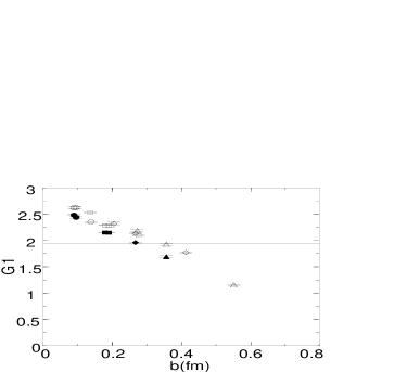
Figure 11: The coupling constant of the monopole self-interaction, $G_{1}$, as a function of the physical length scale $b$. The symbols are: $n=1$ $($$\bullet$$)$, $n=2$ $(\blacksquare)$, $n=3$ $(\blacklozenge)$, $n=4$ $(\blacktriangle)$ for full QCD, and $n=1$ $($$\circ$$)$, $n=2$ $(\square)$, $n=3$ $(\lozenge)$, $n=4$ $(\triangle)$ for quenched QCD.

Our calculations are done on $O(50)$ gauge fixed configurations each on the $24^{3}48$ lattice at $\beta=5.29,\kappa=0.1355$ and on the $16^{3}32$ lattice at $\beta=5.29,\kappa=0.1350$ [8]. For comparison, we have also done calculations in the quenched theory on $24^{3}48$ lattices at $\beta=5.8,6.0$ and $6.2$, and on a $16^{3}32$ lattice at $\beta=6.0$.

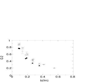
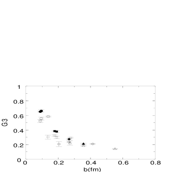
Figure 12: The coupling constants $G_{2}$ and $G_{3}$ as a function of $b$. The symbols are as in Fig. 11.

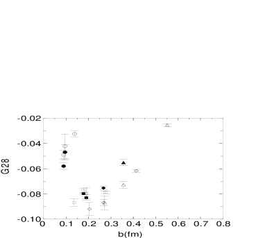
Figure 13: The coupling constants $G_{28}$ and $G_{29}$ of the four-point and six-point interactions, respectively, as a function of $b$. The symbols are as in Fig. 11.

We have employed a type-II block spin transformation [22] with up to $n-1=3$ blocking steps. In Fig. 11 we show the self-coupling $G_{1}$ as a function of the physical length scale $b=na$ for both full and quenched QCD. We see that $G_{1}^{\rm full}$ is systematically smaller than $G_{1}^{\rm quenched}$ for all $b$, in agreement with the higher monopole density in full QCD. A necessary condition for monopole condensation is $G_{1}\leq\ln 7$. This is achieved for $b\gtrapprox 0.27$ fm in full QCD and for $b\gtrapprox 0.35$ fm in the quenched theory. In Fig. 12 we show the coupling constants $G_{2}$ and $G_{3}$. We see that $G_{2}^{\rm full}<G_{2}^{\rm quenched}$ as in the previous case, while $G_{3}$ shows the opposite behavior: $G_{3}^{\rm full}>G(3)^{\rm quenched}$. For the other coupling constants we find little difference between full QCD and the quenched theory. In Fig. 13 we show, as an example, $G_{28}$ and $G_{29}$. Note that the self-coupling is the dominant coupling.

Figure 14: The two-point coupling of monopole currents $k(s,\mu)$ and $k(s^{\prime},\mu)$ as a function of distance $d=\sqrt{\sum_{\mu}(s_{\mu}-s^{\prime}_{\mu})^{2}}$ in full and quenched QCD. The symbols are: full QCD $($$\bullet$$)$, quenched QCD $(\blacksquare)$ and Coulomb propagator $(\lozenge)$.

To shed some more light on the dynamics of the monopoles we have looked at the coupling $G$ of two ($n=1$) parallel monopole currents, $k(s,\mu)$ and $k(s^{\prime},\mu)$, as a function of their distance $d=\sqrt{\sum_{\mu}(s_{\mu}-s^{\prime}_{\mu})^{2}}$. In Fig. 14 we show $G$ together with the Coulomb propagator. We see that at distances $d\gtrapprox 2$ the interaction becomes weaker than Coulomb in both full and quenched QCD. This is a result of the screening effect discussed earlier on. It comes as a surprise though that we see no difference between full QCD and the quenched theory. We would have expected the screening effect to be considerably stronger in full QCD.

Our task for the future is to check for scaling of the effective monopole action, as this has already successfully been done in the quenched theory.

Furthermore, it would be useful to cast the action into the form

$$S(k)=S_{\rm Coulomb}+S_{\rm self}+S_{\rm 4-point}+S_{\rm 6-point},$$

to make contact with the dual Ginzburg-Landau theory, and the string model, and determine their parameters. This would allow us to do truly quantitative, analytic calculations [23].

7 CONCLUSIONS

We have had a first look at the dynamics of color magnetic monopoles in full QCD. We found striking differences between full QCD and the quenched theory.

How can this be understood? Monopoles are at least partly induced by instantons [6, 7]. The fermion determinant causes instantons and anti-instantons to attract each other, with a force that increases with decreasing quark mass. The effect is that isolated instantons are suppressed, and instantons and anti-instantons are forced to form (overlapping) pairs. This will increase the density of (anti-)instantons, and consequently the density of monopoles.

8 ACKNOWLEDGMENTS

This work is partially supported by INTAS grant 00-00111. H.I. is supported by a postdoctoral fellowship of the Japan Society for the Promotion of Science JSPS. She acknowledges the hospitality of the Humboldt-Universität zu Berlin. T.S. acknowledges financial support from a JSPS Grant-in-aid for Scientific Research (B) (No. 11695029).

References

- [1] A.S. Kronfeld, M.L. Laursen, G. Schierholz, U.-J. Wiese, Phys. Lett. B198 (1987) 516.
- [2] H. Shiba, T. Suzuki, Phys. Lett. B333 (1994) 461; J. Stack, S. Neiman, R. Wensley, Phys. Rev. D50 (1994) 3399.
- [3] G.S. Bali, V. Bornyakov, M. Müller-Preussker, K. Schilling, Phys. Rev. D54 (1996) 2863.
- [4] T. Suzuki, in Confinement 2000, p. 120, eds. H. Suganuma, M. Fukushima, H. Toki (World Scientific, Singapore, 2001).
- [5] B. Bakker, M. Chernodub, M. Polikarpov, Phys. Rev. Lett. 80 (1998) 30.
- [6] A. Hart, M. Teper, Phys. Lett. B371 (1996) 261.
- [7] V. Bornyakov, G. Schierholz, Phys. Lett. B384 (1996) 190.
- [8] S. Booth et al, Phys. Lett. B519 (2001) 229.
- [9] F. Brandstaeter, G. Schierholz, U.-J. Wiese, Phys. Lett. B272 (1991) 319.
- [10] G. Bali, V. Bornyakov, M. Müller-Preussker, F. Pahl, Nucl. Phys. B (Proc.Suppl.) 42 (1995) 852.
- [11] T. DeGrand, D. Toussaint, Phys. Rev. D22 (1980) 2478.
- [12] A. Hart, M. Teper, Phys. Rev. D58 (1998) 14504.
- [13] V. Bornyakov, M. Müller-Preussker, these proceedings.
- [14] A. Hasenfratz, Phys. Lett. B476 (2000) 188.
- [15] G.S. Bali, C. Schlichter, K. Schilling, Prog. Theor. Phys. Suppl. 122 (1996) 67.
- [16] M. Lüscher, G. Münster, P. Weisz, Nucl. Phys. B180 (1981) 1.
- [17] G. Bali, hep-ph/9809351.
- [18] P. Olesen, Phys. Lett. B160 (1985) 144.
- [19] N. Arasaki, S. Ejiri, S. Kitahara, Y. Matsubara, T. Suzuki, Phys. Lett. B395 (1997) 275.
- [20] K. Yamagishi, T. Suzuki, S. Kitahara, JHEP 2 (2000) 12.
- [21] H. Shiba, T. Suzuki, Phys. Lett. B343 (1995) 315; ibid. B351 (1995) 519.
- [22] T.L. Ivanenko, A.V. Pochinski, M.I. Polikarpov, Phys. Lett. B252 (1990) 631.
- [23] S. Kato, S. Kitahara, N. Nakamura, T. Suzuki, Nucl. Phys. B 520 (1998) 323; T. Suzuki, these proceedings.