From Spin Ladders to the 2-d $O(3)$ Model at Non-Zero Density

Abstract

The numerical simulation of various field theories at non-zero chemical potential suffers from severe complex action problems. In particular, QCD at non-zero quark density can presently not be simulated for that reason. A similar complex action problem arises in the 2-d $O(3)$ model — a toy model for QCD. Here we construct the 2-d $O(3)$ model at non-zero density via dimensional reduction of an antiferromagnetic quantum spin ladder in a magnetic field. The complex action problem of the 2-d $O(3)$ model manifests itself as a sign problem of the ladder system. This sign problem is solved completely with a meron-cluster algorithm.

1 Introduction

Numerical simulations of numerous quantum systems suffer from notorious sign and complex action problems. For such systems the Boltzmann factor of a configuration in the path integral is in general complex and can hence not be interpreted as a probability. When the complex phase of the Boltzmann factor is incorporated in measured observables, the fluctuations in the phase give rise to dramatic cancellations. In particular, for large systems at low temperatures this leads to relative statistical errors that are exponentially large in both the volume and the inverse temperature. As a consequence, it is impossible in practice to study such systems with standard importance sampling Monte Carlo methods.

Recently, some severe sign problems have been solved with meron-cluster algorithms [1, 2, 3, 4, 5]. Meron-clusters are used to identify canceling pairs of configurations with the same weight but opposite signs. Configurations with merons exactly cancel in the path integral. The Monte Carlo simulation can thus be restricted to the zero-meron sector with positive weights for which standard importance sampling works efficiently.

It is natural to ask if the meron-concept can be applied to the complex action problem in dense QCD. This is indeed the case in the limit of infinitely heavy quarks in the Potts model approximation to QCD [6]. For dynamical light quarks, on the other hand, it is not obvious if the meron concept can be applied to QCD. This seems most likely in the D-theory formulation of field theory in which 4-d QCD arises via dimensional reduction from a $(4+1)$-d quantum link model [7, 8]. Physical gluons emerge as collective excitations of discrete variables [7] — so-called quantum links — which are gauge covariant generalizations of quantum spins. In this paper we study the D-theory formulation of the 2-d $O(3)$ model — a toy model for QCD — which arises via dimensional reduction from an antiferromagnetic spin ladder. In this case, the discrete variables are ordinary quantum spins. At the level of the quantum spin system, the chemical potential of the $O(3)$ model manifests itself as an external magnetic field.

2 Spin Ladders in a Magnetic Field and the 2-d $O(3)$ Model at Non-Zero Density

We consider a ladder system of quantum spins $1/2$ on a square lattice of size $L\times L^{\prime}$ ($L^{\prime}$ even, $L\gg L^{\prime}$) with periodic boundary conditions in both directions. The spins located at the sites $x$ are described by operators ${\bf S}_{x}$ with the usual commutation relations

$$[S_{x}^{i},S_{y}^{j}]=i\delta_{xy}\epsilon_{ijk}S_{x}^{k}.$$ (1)

The antiferromagnetic Hamilton operator ($J>0$)

$$H=J\sum_{x,i}{\bf S}_{x}\cdot{\bf S}_{x+\hat{i}}-{\bf B}\cdot\sum_{x}{\bf S}_{x},$$ (2)

couples the spins at the lattice sites $x$ and $x+\hat{i}$, where $\hat{i}$ is a unit-vector in the $i$-direction.

Chakravarty, Halperin and Nelson used a $(2+1)$-d effective field theory to describe the low-energy dynamics of spatially 2-d quantum antiferromagnets [9]. Chakravarty has applied this theory to quantum spin ladders with a large even number of coupled spin $1/2$ chains [10]. These systems are described by the effective action

$$S[{\bf e}] = \int_{0}^{\beta}dt\int_{0}^{L}dx\int_{0}^{L^{\prime}}dy\ \frac{\rho_{s}}{2}[\partial_{x}{\bf e}\cdot\partial_{x}{\bf e}+\partial_{y}{\bf e}\cdot\partial_{y}{\bf e}$$ (3)

$$+ \frac{1}{c^{2}}\partial_{t}{\bf e}\cdot\partial_{t}{\bf e}],$$

where $\rho_{s}$ is the spin stiffness and $c$ is the spinwave velocity.

When the spin ladder is placed in a uniform external magnetic field ${\bf B}$, the field couples to a conserved quantity — the total spin. Hence, on the level of the effective theory, the magnetic field plays the role of a chemical potential, i.e. it appears as the time-component of an imaginary constant vector potential. As a consequence, the ordinary derivative $\partial_{t}{\bf e}$ is replaced by the covariant derivative $\partial_{t}{\bf e}+i{\bf B}\times{\bf e}$ and the action takes the form

$$S[{\bf e}] = \int_{0}^{\beta}dt\int_{0}^{L}dx\int_{0}^{L^{\prime}}dy\ \frac{\rho_{s}}{2}[\partial_{x}{\bf e}\cdot\partial_{x}{\bf e}+\partial_{y}{\bf e}\cdot\partial_{y}{\bf e}$$ (4)

$$+ \frac{1}{c^{2}}(\partial_{t}{\bf e}+i{\bf B}\times{\bf e})\cdot(\partial_{t}{\bf e}+i{\bf B}\times{\bf e})].$$

For a sufficiently large number of coupled chains ($L^{\prime}\gg c/\rho_{s}$) the system undergoes dimensional reduction to the 2-d $O(3)$ model with the action

$$S[{\bf e}] = \int_{0}^{\beta}dt\int_{0}^{L}dx\ \frac{\rho_{s}L^{\prime}}{2}[\partial_{x}{\bf e}\cdot\partial_{x}{\bf e}$$ (5)

$$+ \frac{1}{c^{2}}(\partial_{t}{\bf e}+i{\bf B}\times{\bf e})\cdot(\partial_{t}{\bf e}+i{\bf B}\times{\bf e})]$$

$$= \int_{0}^{\beta c}d(ct)\int_{0}^{L}dx\ \frac{1}{2g^{2}}[\partial_{x}{\bf e}\cdot\partial_{x}{\bf e}$$

$$+ (\partial_{ct}{\bf e}+i{\bf\mu}\times{\bf e})\cdot(\partial_{ct}{\bf e}+i{\bf\mu}\times{\bf e})].$$

The effective coupling constant is given by $1/g^{2}=\rho_{s}L^{\prime}/c$ and the magnetic field appears as a chemical potential of magnitude $\mu=B/c$.

3 Path Integral for Quantum Magnets

To derive a path integral representation of the partition function we decompose the Hamilton operator of eq.(2) into five terms

$$H=H_{1}+H_{2}+...+H_{5}.$$ (6)

The various terms take the form

$$H_{i}=\!\!\!\sum_{\stackrel{{\scriptstyle x=(x_{1},x_{2})}}{{x_{i}even}}}\!\!\!h_{x,i},\,H_{i+2}=\!\!\!\sum_{\stackrel{{\scriptstyle x=(x_{1},x_{2})}}{{x_{i}odd}}}\!\!\!h_{x,i},$$ (7)

with $h_{x,i}=J{\bf S}_{x}\cdot{\bf S}_{x+\hat{i}}$ and

$$H_{5}=\!\!\!\sum_{\stackrel{{\scriptstyle x=(x_{1},x_{2})}}{{}}}\!\!\!h_{x},$$ (8)

with $h_{x}=-BS_{x}^{1}$. The individual contributions to a given $H_{i}$ commute with each other, but two different $H_{i}$ do not commute. Using the Trotter-Suzuki formula we express the partition function as

$$Z = \mbox{Tr}[\exp(-\beta H)]=\lim_{M\rightarrow\infty}\!\!\!\mbox{Tr}[\exp(-\epsilon H_{1})$$ (9)

$$\times \exp(-\epsilon H_{2})...\exp(-\epsilon H_{5})]^{M}.$$

We have introduced $5M$ Euclidean time slices with $\epsilon=\beta/M$ as the lattice spacing in the Euclidean time direction. We insert complete sets of eigenstates $|\uparrow\rangle$ and $|\downarrow\rangle$ with eigenvalues $S_{x}^{3}=\pm 1/2$ between the factors $\exp(-\epsilon H_{i})$.

The partition function is now expressed as a path integral

$$Z=\sum_{s}\mbox{Sign}[s]\exp(-S[s]),$$ (10)

over configurations of spins $s(x,t)=\uparrow,\downarrow$ on a $(2+1)$-dimensional space-time lattice of points $(x,t)$. The Boltzmann factor $\exp(-S[s])$ is a product of space-time plaquette contributions $\exp\{-S[s(x,t),s(y,t),s(x,t+1),s(y,t+1)]\}$ with

$$\exp(-S[\uparrow,\uparrow,\uparrow,\uparrow]) = \exp(-S[\downarrow,\downarrow,\downarrow,\downarrow])=$$

$$= \exp(-\epsilon J/2),$$

$$\exp(-S[\uparrow,\downarrow,\uparrow,\downarrow]) = \exp(-S[\downarrow,\uparrow,\downarrow,\uparrow])=$$

$$= \cosh(\epsilon J/2),$$

$$\exp(-S[\uparrow,\downarrow,\downarrow,\uparrow]) = \exp(-S[\downarrow,\uparrow,\uparrow,\downarrow])=$$ (11)

$$= \sinh(\epsilon J/2),$$

as well as the time-like bond contributions $\exp\{-S[s(x,t),s(x,t+1)]\}$ with

$$\exp(-S[\uparrow,\uparrow])=\exp(-S[\downarrow,\downarrow])=\cosh(\epsilon B/2),$$

$$\exp(-S[\uparrow,\downarrow])=\exp(-S[\downarrow,\uparrow])=\sinh(\epsilon B/2).$$ (12)

The sign of a configuration, $\mbox{Sign}[s]$, also is a product of space-time plaquette contributions $\mbox{Sign}[s(x,t),s(y,t),s(x,t+1),s(y,t+1)]$ with

$$\mbox{Sign}[\uparrow,\uparrow,\uparrow,\uparrow])=\mbox{Sign}[\downarrow,\downarrow,\downarrow,\downarrow])=1,$$

$$\mbox{Sign}[\uparrow,\downarrow,\uparrow,\downarrow])=\mbox{Sign}[\downarrow,\uparrow,\downarrow,\uparrow])=1,$$

$$\mbox{Sign}[\uparrow,\downarrow,\downarrow,\uparrow])=\mbox{Sign}[\downarrow,\uparrow,\uparrow,\downarrow])=-1.$$ (13)

Figure 1 shows two spin configurations in $(1+1)$ dimensions. The first configuration is completely antiferromagnetically ordered and has $\mbox{Sign}[s]=1$. The second configuration contains one interaction plaquette with configuration $[\downarrow,\uparrow,\uparrow,\downarrow]$ which contributes $\mbox{Sign}[\downarrow,\uparrow,\uparrow,\downarrow]=-1$, such that the whole configuration has $\mbox{Sign}[s]=-1$.

The central observable of our study is the uniform magnetization ${\bf M}=\sum_{x}{\bf S}_{x}$.

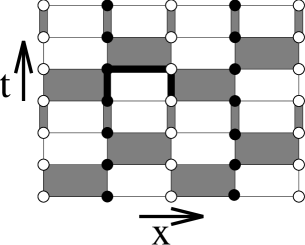
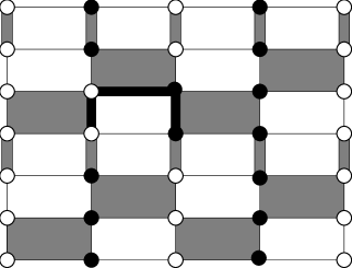
Figure 1: Two spin configurations in $(1+1)$ dimensions. The shaded plaquettes and time-like bonds carry the interaction. Filled dots represent spin up and open circles represent spin down. The first configuration has $\mbox{Sign}[s]=1$ and the second configuration has $\mbox{Sign}[s]=-1$. The fat black line represents a meron-cluster. The other clusters are not shown. Flipping the meron-cluster changes one configuration into the other and changes $\mbox{Sign}[s]$.

4 Meron-Cluster Algorithm

The meron-cluster algorithm is based on a cluster algorithm for a modified model without the sign factor. Quantum spin systems without a sign problem can be simulated very efficiently with the loop-cluster algorithm [11, 12, 13, 14]. The idea behind the algorithm is to decompose a configuration into clusters which can be flipped independently. Each lattice site belongs to exactly one cluster. When the cluster is flipped, the spins at all the sites on the cluster are changed from up to down and vice versa. The decomposition of the lattice into clusters results from connecting neighboring sites on each space-time interaction plaquette or time-like interaction bond according to probabilistic cluster rules. A set of connected sites defines a cluster. In this case the clusters are open or closed strings. The cluster rules are constructed so as to obey detailed balance. To show this property we first write the space-time plaquette Boltzmann factors as

$$\exp(-S[s(x,t),s(y,t),s(x,t+1),s(y,t+1)])=$$

$$A\delta_{s(x,t),s(x,t+1)}\delta_{s(y,t),s(y,t+1)}+$$

$$B\delta_{s(x,t),-s(y,t)}\delta_{s(x,t+1),-s(y,t+1)}.$$ (14)

The $\delta$-functions specify which sites are connected and thus belong to the same cluster. The coefficients $A$ and $B$ determine the relative probabilities for different cluster break-ups of an interaction plaquette. For example, $A$ determines the probability with which sites are connected with their time-like neighbors and $B$ determines the probability for connections with space-like neighbors. Inserting the expressions from eq.(3) one finds

$$\exp(-S[\uparrow,\uparrow,\uparrow,\uparrow]) = \exp(-S[\downarrow,\downarrow,\downarrow,\downarrow])=$$

$$= \exp(-\epsilon J/2)=A,$$

$$\exp(-S[\uparrow,\downarrow,\uparrow,\downarrow]) = \exp(-S[\downarrow,\uparrow,\downarrow,\uparrow])=$$

$$= \cosh(\epsilon J/2)=A+B,$$

$$\exp(-S[\uparrow,\downarrow,\downarrow,\uparrow]) = \exp(-S[\downarrow,\uparrow,\uparrow,\downarrow])=$$ (15)

$$= \sinh(\epsilon J/2)=B.$$

Similarly, the time-like bond Boltzmann factors are expressed as

$$\exp(-S[s(x,t),s(x,t+1)])=$$

$$C\delta_{s(x,t),s(x,t+1)}+D.$$ (16)

The probability to connect spins with their time-like neighbors is $C/(C+D)$. The spins remain disconnected with probability $D/(C+D)$. Inserting the expressions from eq.(3) one obtains

$$\exp(-S[\uparrow,\uparrow]) = \exp(-S[\downarrow,\downarrow])=$$

$$= \cosh(\epsilon B/2)=C+D,$$

$$\exp(-S[\uparrow,\downarrow]) = \exp(-S[\downarrow,\uparrow])=$$ (17)

$$= \sinh(\epsilon B/2)=D.$$

The cluster rules are illustrated in table 1.

configuration	break-ups
	A
	$\begin{array}[]{c}\hskip 11.38092pt\begin{minipage}[c]{71.13188pt} \vbox{\begin{center} \psfig{width=42.67912pt,angle=270,bbllx=-20,bblly=0,bburx=55,bbury=85} \par\vspace{0.1cm}A \end{center}} \end{minipage}\\ \hskip 11.38092pt\begin{minipage}[c]{71.13188pt} \vbox{\begin{center} \psfig{width=42.67912pt,angle=270,bbllx=-20,bblly=0,bburx=55,bbury=85} \par\vspace{0.1cm}B \end{center}} \end{minipage}\end{array}$
	B
	C                       D
	D

Table 1: Cluster break-ups of various plaquette and time-like bond configurations together with their relative probabilities $A,B,C,D$. Filled dots represent spin up, open circles represent spin down, and the fat lines are the cluster connections.

Eqs.(4,4) can be viewed as a representation of the original model as a random cluster model. The cluster algorithm operates in two steps. First, a cluster break-up is chosen for each space-time interaction plaquette or time-like interaction bond according to the above probabilities. This effectively replaces the original Boltzmann weight of a configuration with a set of constraints represented by the $\delta$-functions associated with the chosen break-ups. The constraints imply that the spins in one cluster can only be flipped together. Second, every cluster is flipped with probability $1/2$. When a cluster is flipped, the spins on all sites that belong to the cluster are flipped from up to down and vice versa. Eqs.(4,4) ensure that the cluster algorithm obeys detailed balance.

The above cluster rules were first used in a simulation of the Heisenberg antiferromagnet [12] in the absence of a magnetic field. In that case there is no sign problem. Then the corresponding loop-cluster algorithm is extremely efficient and has almost no detectable autocorrelations. When a magnetic field is switched on the situation changes. When the magnetic field points in the direction of the spin quantization axis (the $3$-direction in our case) there is no sign problem. However, the magnetic field then explicitly breaks the ${\sf Z\!\!\!Z}(2)$ flip symmetry on which the cluster algorithm is based, and the clusters can no longer be flipped with probability $1/2$. Instead the flip probability is determined by the value of the magnetic field and by the magnetization of the cluster. When the field is strong, flips of magnetized clusters are rarely possible and the algorithm becomes inefficient. To avoid this, we have chosen the magnetic field to point in the $1$-direction, i.e. perpendicular to the spin quantization axis. In that case, the cluster flip symmetry is not affected by the magnetic field, and the clusters can still be flipped with probability $1/2$. However, one now faces a sign problem and the cluster algorithm becomes extremely inefficient again. Fortunately, using the meron concept the sign problem can be eliminated completely and the efficiency of the original cluster algorithm can be maintained even in the presence of a magnetic field.

5 Meron-Clusters and the Sign Problem

Let us consider the effect of a cluster flip on the sign. The flip of a meron-cluster changes $\mbox{Sign}[s]$, while the flip of a non-meron-cluster leaves $\mbox{Sign}[s]$ unchanged. An example of a meron-cluster is shown in figure 1. When the meron cluster is flipped, the first configuration with $\mbox{Sign}[s]=1$ turns into the second configuration with $\mbox{Sign}[s]=-1$. This property of the cluster is independent of the orientation of any other cluster. Since flipping all spins leaves $\mbox{Sign}[s]$ unchanged, the total number of meron-clusters is always even.

The meron concept allows us to gain an exponential factor in statistics. Since all clusters can be flipped independently with probability $1/2$, one can construct an improved estimator for $\langle\mbox{Sign}\rangle$ by averaging analytically over the $2^{N_{C}}$ configurations obtained by flipping the $N_{C}$ clusters in a configuration in all possible ways. For configurations that contain merons, the average $\mbox{Sign}[s]$ is zero because flipping a single meron-cluster leads to a cancellation of contributions $\pm 1$. Hence only the configurations without merons contribute to $\langle\mbox{Sign}\rangle$. The probability for having a configuration without merons is equal to $\langle\mbox{Sign}\rangle$ and is exponentially suppressed with the space-time volume. The vast majority of configurations contains merons and contributes an exact $0$ to $\langle\mbox{Sign}\rangle$ instead of a statistical average of contributions $\pm 1$. In this way the improved estimator leads to an exponential gain in statistics. One can show that the contributions from the zero-meron sector are always positive.

One can also find a simple expression for the improved estimator for the magnetization $\langle M^{1}\rangle$ in terms of a winding number $W_{l}$ of closed loops which result from joining open string clusters. One can define $W_{l}$ for each loop to be its temporal winding number. If a particular loop is not composed of open string clusters then $W_{l}=0$. With this definition of $W_{l}$ it is easy to show that

$$\langle M^{1}\rangle=\frac{\langle\delta_{N,0}\sum_{l}W_{l}\rangle}{2\langle\delta_{N,0}\rangle},$$ (18)

where $N$ is the number of meron-clusters.

Since the magnetization gets non-vanishing contributions only from the zero-meron sector, it is unnecessary to generate any configuration that contains meron-clusters. This observation is the key to the solution of the sign problem. In fact, one can gain an exponential factor in statistics by restricting the simulation to the zero-meron sector, which represents an exponentially small fraction of the whole configuration space. We visit all plaquette and time-like bond interactions one after the other and choose new pair connections between the sites according to the above cluster rules. A newly proposed pair connection that takes us out of the zero-meron sector is rejected. After visiting all plaquette and time-like bond interactions, each cluster is flipped with probability $1/2$ which completes one update sweep. In practice, it is advantageous to occasionally generate configurations containing merons even though they do not contribute to our observable, because this reduces the autocorrelation times.

Figure 2 shows the magnetization density of antiferromagnetic quantum spin ladders with $L^{\prime}=4$ compared to analytic results (valid for large $L^{\prime}$) obtained with the Bethe ansatz [15] using the massgap $m=0.141(2)/a$ [16] and the spinwave velocity $c=1.657(2)Ja$ [17]. The agreement is remarkable and involves no adjustable free parameters.

Figure 2: Magnetization density $\langle M^{1}\rangle/L$ of quantum spin ladders consisting of $L^{\prime}=4$ coupled chains as a function of the magnetic field $B$. The numerical data are for two systems: one of size $L=20$ at inverse temperature $\beta J=15$ (circles) and the other for $L=40$ at $\beta J=24$ (diamonds). The solid curve is the infinite volume, zero temperature analytic result, while the two dashed curves are finite volume, non-zero temperature analytic results for the two simulated systems in the intermediate $B$ region. The dotted curve represents saturation of the magnetization per spin at $1/2$.

6 Conclusions

Using D-theory, the 2-d $O(3)$ model at non-zero chemical potential has been obtained from dimensional reduction of a $(2+1)$-d quantum spin ladder in a magnetic field. The resulting sign problem has been solved completely with a meron-cluster algorithm. This is the first time that this toy model for QCD has been simulated efficiently at non-zero chemical potential. The next challenge is to address the complex action problem of dense QCD. In D-theory quarks arise as domain wall fermions and gluons emerge as collective excitations of quantum links. Hence, one needs to generalize the meron-concept to quantum link models as well as to domain wall fermions.

References

- [1] W. Bietenholz, A. Pochinsky and U.-J. Wiese, Phys. Rev. Lett. 75 (1995) 4524.
- [2] S. Chandrasekharan and U.-J. Wiese, Phys. Rev. Lett. 83 (1999) 3116.
- [3] S. Chandrasekharan, J. Cox, K. Holland and U.-J. Wiese, Nucl. Phys. B576 (2000) 481.
- [4] J. Cox, C. Gattringer, K. Holland, B. Scarlet and U.-J. Wiese, Nucl. Phys. (Proc. Suppl.) 83 (2000) 777.
- [5] S. Chandrasekharan and J. Osborn, cond-mat/0109424.
- [6] M. Alford, S. Chandrasekharan, J. Cox and U.-J. Wiese, Nucl. Phys. B602 (2001) 61.
- [7] S. Chandrasekharan and U.-J. Wiese, Nucl. Phys. B492 (1997) 455.
- [8] R. Brower, S. Chandrasekharan and U.-J. Wiese, Phys. Rev. D60 (1999) 094502.
- [9] S. Chakravarty, B. I. Halperin and D. R. Nelson, Phys. Rev. Lett. 60 (1988) 1057; Phys. Rev. B39 (1989) 2344.
- [10] S. Chakravarty, Phys. Rev. Lett. 77 (1996) 4446.
- [11] H. G. Evertz, G. Lana and M. Marcu, Phys. Rev. Lett. 70 (1993) 875.
- [12] U.-J. Wiese and H.-P. Ying, Z. Phys. B93 (1994) 147.
- [13] H. G. Evertz, The loop algorithm, in Numerical Methods for Lattice Quantum Many-Body Problems, ed. D. J. Scalapino, Addison-Wesley Longman, Frontiers in Physics.
- [14] B. B. Beard and U.-J. Wiese, Phys. Rev. Lett. 77 (1996) 5130.
- [15] P. B. Wiegmann, Phys. Lett. B152 (1985) 209.
- [16] O. F. Syljuasen, S. Chakravarty and M. Greven, Phys. Rev. Lett. 78 (1997) 4115.
- [17] B. B. Beard, R. J. Birgeneau, M. Greven and U.-J. Wiese, Phys. Rev. Lett. 80 (1998) 1742.