Generalized ensemble algorithm for U(1) gauge theory

Abstract

Hybrid Monte Carlo simulations of the pure compact U(1) gauge theory are performed with the Tsallis weight. The simulations show that the use of the Tsallis weight enhances the tunneling rate between metastable states.

1 INTRODUCTION

The four dimensional pure compact U(1) gauge theory is known to posses a phase transition (PT) separating a confined phase and a Coulomb one and the determination of the order of PT is of great importance. In the pure compact U(1) gauge theory, however, the determination of the order of PT is very difficult since on large lattices the standard updating algorithms like Metropolis, heat-bath, hybrid Monte Carlo (HMC)[1], fail to generate enough tunneling between metastable states. Many efforts have been done to clarify the order of the PT[2]. In spite of such efforts the order of the PT is still controversial.

A promising algorithm to overcome this difficulty is the multicanonical algorithm[3] which uses a multicanonical weight in stead of the Boltzmann one and can enhance the tunneling rate between metastable states. Although the multicanonical algorithm works effectively, one disadvantage of the multicanonical algorithm might be that a multicanonical weight used in the simulations is not known a priori and it must be determined before the simulations. Usually the weight is estimated from a short run of the standard updating algorithm. However this estimation is more difficult as a lattice size becomes larger.

Recently in several fields where the usual Monte Carlo technique does not work effectively, simulations were performed with the Tsallis weight[4, 5], first introduced by Tsallis[6]. The Tsallis weight controlled by a parameter $q$ can be easily defined, and the usual Boltzmann weight is given by taking the limit $q\rightarrow 1$. The results have showed that the use of the Tsallis weight might be more advantageous than that of the Boltzmann one.

Inspired by such studies, here we apply the Tsallis weight for the hybrid Monte Carlo simulation of the pure compact U(1) lattice gauge theory and investigate whether the Tsallis weight solves the difficulty in determining the order of the PT.

2 GENERALIZED ENSEMBLE AND TSALLIS WEIGHT

The partition function of a system with the action $S$ is given by

$$Z=\int\exp(-\beta S[U])dU.$$ (1)

Introducing a function $G$, the partition function can be rewritten as

$$Z = \int\exp(-\beta S[U])/G\cdot GdU$$ (2)

$$= <\frac{\exp(-\beta S)}{G}>_{G}Z_{G},$$

where $Z_{G}$ is a generalized partition function:

$$Z_{G}=\int GdU,$$ (3)

and $<O>_{G}$ stands for the expectation value of an observable $O$ in the ensemble generated with $Z_{G}$. The expectation value of $O$ in the canonical ensemble generated with eq.(1) can be obtained in terms of the generalized ensemble as

$$<O> = \int O\exp(-\beta S[U])dU/Z$$ (4)

$$= <O\frac{e^{-\beta S}}{G}>_{G}/<\frac{e^{-\beta S}}{G}>_{G}.$$

Previously it was suggested that in some cases Tsallis weight works better than the Boltzmann one[4, 5]. In the Tsallis formulation,

$$G=[1-(1-q)\beta\bar{S}]^{\frac{1}{(1-q)}},$$ (5)

or in the familiar exponential form,

$$G=\exp(-\beta S_{T})\equiv W_{T},$$ (6)

with

$$S_{T}=\frac{1}{\beta(q-1)}\ln[1-(1-q)\beta\bar{S}],$$ (7)

where $\bar{S}=S-S_{0}$. $S_{0}$ is a certain constant shifting the origin of the action. Here we call $W_{T}$ ”Tsallis weight”. The Boltzmann weight can be obtained by taking the limit $q\rightarrow 1$ in the Tsallis weight $W_{T}$.

3 Hybrid Monte Carlo with Tsallis weight

The action of pure compact U(1) lattice gauge theory is given by

$$S=\sum_{x,\mu>\nu}[1-\cos(\theta_{\mu\nu}(x))],$$ (8)

where $\theta_{\mu\nu}(x)$ is the sum of link angles contributing a plaquette at a site $x$ on the $\mu\nu$ plane. The Hamiltonian with the Tsallis weight, used for HMC simulations, is defined by

$$H_{T}=\sum\frac{1}{2}p^{2}_{i}+\beta S_{T}.$$ (9)

Here note that $S_{T}$ is not always well-defined. Namely $1-(1-q)\beta\bar{S}$ can be negative. However, provided that $q$ is close to one, $1-(1-q)\beta\bar{S}$ is made positive.

4 RESULTS

As an exploratory study we tested the above algorithm varying $q$ on an $8^{4}$ lattice in the vicinity of the PT ( at $\beta=1.00737$ ). We performed HMC simulations[1] with eq.(9). $S_{0}$ ( = 0.37 ) was taken to be the average value of the action $S$. In order to make comparisons, we also performed HMC simulations with the Boltzmann weight. Typically we simulated $10^{6}$ trajectories for each $q$.

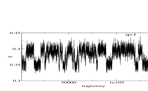
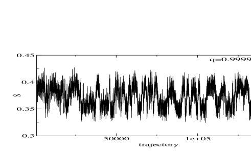
Figure 1: (top): Typical history of action $S$ for $q=1$ ( Boltzmann weight ). (bottom): $S_{T}$ for q=0.99997.

We observed more tunneling for $q<1$ than for $q=1$ (the Boltzmann weight). Fig.1 shows representative history of actions of q=1 and 0.999997 and we see more tunneling for the case of q=0.999997.

Fig.2 shows action densities of q=1, 0.999997, 0.999995 and 0.99999. The height of the valley between two peaks increases as $q$ decreases which indicates that the tunneling rate increases as $q$ decreases. For too small $q$, however, values of the action will locate near $S_{0}$ and in this case there may be a difficulty in reweighting. Fig.3 and 4 show that the action densities reweighted to q=1 and compare those with the Boltzmann action density ( $q=1$ ). The reweight densities reproduce well the Boltzmann action density. However, for $q=0.99999$ ( the smallest $q$ here ) the reweighted action density has large fluctuations at $S$ far from $S_{0}$, which may indicate that one needs caution when using the Tsallis weight.

It is also possible to take $q>1$ in the simulations. For $q>1$, however, the desired behavior, i.e. more tunneling, was never observed for our case.

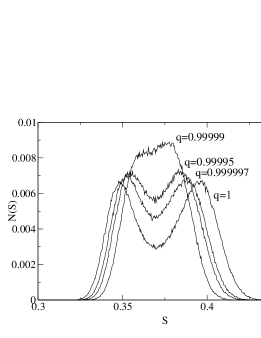
Figure 2: The action densities $N(S)$ for q=1, 0.99997,0.999995 and 0.99999

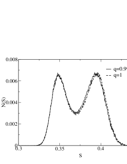
Figure 3: Comparison between the action density of $q=1$ and the reweighted action density of $q=0.999997$.

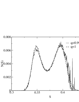
Figure 4: Comparison between the action density of $q=1$ and the reweighted action density of $q=0.99999$.

5 DISCUSSION

The exploratory study on an $8^{4}$ lattice showed that the Tsallis weight enhances the tunneling rate. The lattice size used here is small. For precise determination of the order of the PT, larger lattices are needed. Therefore it is important to confirm that this preferred feature of the Tsallis weight is preserved for larger lattices, possibly up to $18^{4}$ lattice size or so. Simulations on larger lattices are in progress.

References

- [1] S.Duane et. al, Phys. Lett. B195 (1987) 216
- [2] B.Lautrup and M.Nauenberg, Phys. Lett. B95 (1980) 63; G.Bhanot, Phys. Rev. D24 (1981) 461; K.-H.Mëtter and K.Schilling, Nucl. Phys. B200 (1982) 362; R.Gupta, A.Movotny and P.M.Zerwas, Phys. Lett. B133 (1983) 103; V.Azcoiti, G. di Carlo and A.Grillo, Phys. Lett. B268 (1991) 101; G.Bhanot, Th.Lippert, K.Schilling and P.Ueberholz, Nucl. Phys. B378 (1992) 633; B.Klaus and C.Roiesnel, Phys. Rev. D58 (1997) 114509
- [3] B.A.Berg and T.Neuhaus, Phys. Lett. B267 (1991) 249; G.Arnold, K.Schilling and Th. Lippert, Phys. Rev. D 59 (1999) 054509
- [4] U.H.E.Hansmann, F.Eisenmenger and Y.Okamoto, physics/9810052
- [5] M.Iwamatsu and Y.Okabe, cond-mat/0001220
- [6] C.Tsallis, J. Stat. Phys. 52 (1988) 479