Dynamical Fermions in Hamiltonian Lattice Gauge Theory

Abstract

We describe a first attempt to understand dynamical fermions within a Hamiltonian framework.  As a testing ground we study compact QED₃, which shares some important features of QCD₄ such as confinement, glueballs, mesons, and chiral symmetry breaking.  We discuss the methods used and show data for the chiral condensate.

1 Introduction

Nearly all lattice studies with dynamical fermions rely on pseudofermion techniques.  This includes the standard Hybrid Monte Carlo method for non-local boson actions [1] and more recently multiboson methods proposed by Lüscher [2] and extended to odd flavors by Boriçi and de Forcrand [3]. While these methods are presently the most efficient available for dynamical fermion calculations, much improvement is still needed to combat algorithmic slowdown at light quark masses and large volumes.  On the more theoretical side, one would also like to understand the microscopic dynamics of quarks in lattice simulations.  Ideally one hopes to see the effects of confinement on quark-antiquark pair separation and the effects of chiral symmetry breaking on light quark mobility.  These questions are most easily answered in a framework which does not integrate out the fermionic degrees of freedom.  With these goals in mind we investigate the possibility of simulating dynamical fermions in a confining gauge theory with explicit fermion dynamics.

In this proceedings article we describe the beginning of a research program at NC State to understand dynamical fermions within a Hamiltonian framework.  As a testing ground we study compact QED₃, which exhibits confinement, glueballs, mesons, and chiral symmetry breaking.  We discuss the methods that are being used and show preliminary data for the chiral condensate and compare with strong and weak coupling results.

2 Compact QED₃

We follow the notation used in [4] and [5].  The Hamiltonian is

$$H=\tfrac{1}{2a\sqrt{x}}W\text{,}$$ (1)

where $a$ is the lattice spacing and $x$ the dimensionless strong coupling constant,

$$x=e^{-4}a^{-2}\text{.}$$ (2)

$W$ has three pieces,

$$W=W_{0}+\sqrt{x}W_{1}+xW_{2}\text{,}$$ (3)

where

$$W_{0} =\sum_{l}E_{l}^{2}-\mu\sum_{\vec{r}}(-1)^{r_{1}+r_{2}}\chi^{\dagger}(\vec{r})\chi(\vec{r})$$ (4)

$$W_{1} =\sum_{\vec{r},j}\eta_{j}(\vec{r})\left[\chi^{\dagger}(\vec{r})U_{j}(\vec{r})\chi(\vec{r}+\hat{\jmath})+\text{h.c.}\right]$$

$$W_{2} =-\sum_{p}\left(U_{p}+U_{p}^{\dagger}\right)$$

and $\eta_{1}(\vec{r})=(-1)^{r_{2}+1}$, $\eta_{2}(\vec{r})=1$. We use four component staggered fermions, which in the three-dimensional Hamiltonian formalism gives one flavor of fermion.  The dimensionless mass parameter $\mu$ is given by

$$\mu=2me^{-2}\text{.}$$ (5)

3 Methods

We start with a set of trial states $\left|\Psi_{j}\right\rangle$ and evaulate the quantities

$$M_{ij} =\left\langle\Psi_{i}\right|\exp\left[-HT\right]\left|\Psi_{j}\right\rangle,$$ (6)

$$M_{ij}^{\Delta} =\left\langle\Psi_{i}\right|\exp\left[-H(T+\Delta T)\right]\left|\Psi_{j}\right\rangle.$$

Improved trial states are given by

$$\left|\Psi_{j}^{\prime}\right\rangle=\exp[-\tfrac{1}{2}HT]\left|\Psi_{j}\right\rangle.$$ (7)

It is easy to see that

$$M_{ij} =\left\langle\Psi_{j}^{\prime}\right.\left|\Psi_{j}^{\prime}\right\rangle,$$ (8)

$$M_{ij}^{\Delta} =\left\langle\Psi_{j}^{\prime}\right|\exp\left[-H\Delta T\right]\left|\Psi_{j}^{\prime}\right\rangle.$$ (9)

We now find a matrix $T$ and unitary matrix $U$ such that

$$T_{ij}^{\dagger}M_{jk}T_{kl} =\delta_{il},$$ (10)

$$U_{ij}^{\dagger}T_{jk}^{\dagger}M_{kl}^{\Delta}T_{lm}U_{mn} =\lambda_{i}\delta_{in}.$$

From these we can read off approximate eigenvectors

$$\left|E_{l}\right\rangle=T_{lm}U_{mj}\left|\Psi_{j}^{\prime}\right\rangle$$ (11)

and eigenvalues

$$\left|E_{l}\right\rangle=-\tfrac{1}{\Delta T}\log\lambda_{l}\text{.}$$ (12)

The matrices $M$ and $M^{\Delta}$ are evaluated by dividing into time slices,

$$M_{ij}=\left\langle\Psi_{j}^{\prime}\right|\exp\left[-\tfrac{HT}{N}\right]\cdots\exp\left[-\tfrac{HT}{N}\right]\left|\Psi_{j}^{\prime}\right\rangle\text{.}$$ (13)

Between the time slices we insert a complete set of states, and the basis we choose is the tensor product basis of gauge and fermion states.  For the gauge states we use coherent states of the link fields,

$$U_{j}(\vec{x}){\textstyle\bigotimes_{l,\vec{r}}}\left|A_{l}(\vec{r})\right\rangle =e^{iA_{j}(\vec{x})}{\textstyle\bigotimes_{l,\vec{r}}}\left|A_{l}(\vec{r})\right\rangle$$ (14)

$$U_{j}^{\dagger}(\vec{x}){\textstyle\bigotimes_{l,\vec{r}}}\left|A_{l}(\vec{r})\right\rangle =e^{-iA_{j}(\vec{x})}{\textstyle\bigotimes_{l,\vec{r}}}\left|A_{l}(\vec{r})\right\rangle.$$

For the fermion states we use the usual position-space basis.  For fixed coherent states of the gauge field between time slices, the fermion dynamics are generated a classical background field,

$$\chi^{\dagger}(\vec{r})U_{j}(\vec{r})\chi(\vec{r}+\hat{\jmath})\rightarrow e^{iA_{j}(\vec{r})}\chi^{\dagger}(\vec{r})\chi(\vec{r}+\hat{\jmath}).$$ (15)

4 Simulations

In our calculations we keep the lowest few energy fermionic states in computer memory and calculate their dynamics exactly by matrix multiplication.  We use a simple heat bath algorithm to propose new gauge updates.  These updates are performed by sweeps through the spatial lattice, taking each time slice in succession.  We use a Metropolis accept/reject decision based upon an estimator that includes the contribution of the low energy fermion states.  In comparison with quenched simulations, the use of this estimator is slower by a constant factor proportional to the number of low energy fermion states.  After each sweep through all time slices, the contribution of other fermionic states are calculated using diffusion Monte Carlo sampling.

In our initial studies of small to mid-sized lattices we store in memory the nine lowest energy fermion states in memory, the strong coupling ground state and the eight translationally invariant states connected to the ground state by a single hop.  In Figure 1 we show results for $\mu=2$.  The data is extrapolated from spatial lattice sizes $4\times 4$, $8\times 8$, and $10\times 10$, and number of time slices $11$, $15$, and $19$.  The curves $s_{0},s_{1},s_{2},s_{3}$ give the first few orders in the strong coupling expansion, and $w$ is the leading behavior in the weak coupling expansion.  We find behavior consistent with strong coupling estimates at small $x$ and weak coupling estimate at large $x$.

5 Conclusions

We have described a first attempt to treat dynamical fermions within a Hamiltonian framework.  We considered compact QED₃, which shares some important features of QCD₄.  At this time it is too early to say whether this approach would be viable for QCD₄ with relatively light quarks.  We are currently making accuracy and efficiency comparisons with pseudofermion methods in QED₃ [6] for exactly massless fermions.

On the theoretical side there is clearly much potential in this approach to better understand the microscopic dynamics of quarks in lattice simulations.  In future work we plan to study the effects of confinement and chiral symmetry breaking on quark dynamics.

The author thanks Pieter Maris and Nathan Salwen for discussions.

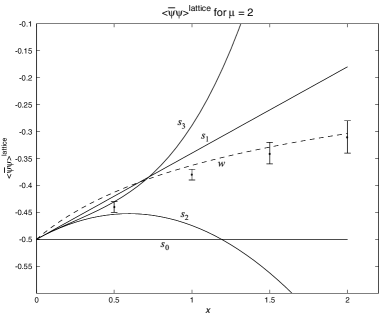
Figure 1: Chiral condensate for $\mu=2$. $s_{0,}s_{1},s_{2},s_{3}$ represent the lowest order estimates in the strong coupling expansion, and $w$ is the leading result in the weak coupling expansion.

References

- [1] S. Duane, A. Kennedy, B. Pendleton, D. Roweth, Phys. Lett. B195 (1987) 216.
- [2] M. Lüscher, Nucl. Phys. B418 (1994) 637.
- [3] A. Boriçi, P. de Forcrand, Nucl. Phys. B454 (1995) 645.
- [4] C. Burden, C. Hamer, Phys. Rev. D37 (1998) 479.
- [5] C. Hamer, J. Oitmaa, Z. Weihong, Phys. Rev. D57 (1998) 2523.
- [6] A. Burkitt, A. Irving, Nucl. Phys. B295 (1988) 525