Quenched Results for Light Quark Physics with Overlap Fermions

Abstract

We present results of a quenched QCD simulation with overlap fermions on a lattice of volume $V=16^{3}\times 32$ at $\beta=6.0$, which corresponds to a lattice cutoff of $\simeq 2$ GeV and an extension of $\simeq 1.4$ fm. From the two-point correlation functions of bilinear operators we extract the pseudoscalar meson masses and the corresponding decay constants. From the GMOR relation we determine the chiral condensate and, by using the $K$-meson mass as experimental input, we compute the sum of the strange and average up-down quark masses $(m_{s}+\hat{m})$. The needed logarithmic divergent renormalization constant $Z_{S}$ is computed with the RI/MOM non-perturbative renormalization technique. Since the overlap preserves chiral symmetry at finite cutoff and volume, no divergent quark mass and chiral condensate additive renormalizations are required and the results are ${\cal O}(a)$ improved.

1 Introduction

In the last few years a major breakthrough in the lattice regularization of Fermi fields was achieved through the closely related domain wall [1] and overlap [2] formulations. Neuberger found a lattice Dirac operator $D$ [3] which avoids doubling and, most notably, satisfies the Ginsparg-Wilson (GW) relation [4]. Thus the corresponding action in the massless limit preserves a lattice form of chiral symmetry at finite lattice spacing and volume [3, 5]. As a result the use of the overlap action entails many theoretical advantages (see ref. [6] and references therein for recent reviews); in particular it forbids mixing among operators of different chirality and therefore it can be very helpful (if not crucial) for computing weak amplitudes. No power-divergent subtractions are needed to calculate the matrix elements relevant for the $\Delta I=1/2$ rule in $K\rightarrow\pi\pi$ decays [7].

The theoretical advantages of overlap fermions come at the cost of an increased computational burden in numerical simulations. The main question we wish to answer in the work presented here is whether the overlap formalism can be effectively used for large scale QCD calculations, with known algorithms and the current generation of computers. The calculation of light quark masses is an ideal test since it uses many of the ingredients needed for a generic phenomenological computation.

We have performed a fully non-perturbative calculation of $(m_{s}+\hat{m})$ in the quenched approximation following the procedure proposed in [8]. We also report results for the chiral condensate computed using the Gell-Mann–Oakes–Renner (GMOR) relation and for the pseudoscalar meson masses and decay constants.

2 Quark Masses and Chiral Condensate

The fermionic action in the overlap regularization reads

$$S=\bar{\psi}\left[\Big{(}1-\frac{1}{2\rho}aM\Big{)}D+M\right]\,\psi$$ (1)

where $M$ is the matrix of bare masses $(m_{1},m_{2},\dots)$ in flavor space. The Neuberger-Dirac operator is defined as [3]

$$D = \frac{\rho}{a}\left(1+V\right)=\frac{\rho}{a}\left(1+X\frac{1}{\sqrt{X^{\dagger}X}}\right)$$ (2)

$$X = D_{W}-\frac{1}{a}\rho\,$$ (3)

where $D_{W}$ is the Wilson-Dirac operator (definitions and conventions used here are fully described in ref. [9]). The renormalized quark mass is defined as

$$\hat{m}(\mu)=\lim_{a\rightarrow 0}Z_{m}(a\mu)m(a)$$ (4)

where $Z_{m}(a\mu)$ is a logarithmically divergent renormalization constant and $m(a)$ is the bare mass parameter which appears in the action of eq. (1) and in the corresponding axial and vector Ward identities. The non-singlet “local” bilinear quark operators we are interested in are defined as

$$O_{\Gamma}(x)=\bar{\psi}_{1}(x)\Gamma\left[(1-\frac{a}{2\rho}D)\psi_{2}\right](x)$$ (5)

where $O_{\Gamma}\equiv\{V_{\mu},A_{\mu},S,P\}$ correspond to $\Gamma\equiv\{\gamma_{\mu},\gamma_{\mu}\gamma_{5},\hbox{1$\!\!$1},\gamma_{5}\}$. They are subject to multiplicative renormalization only, i.e. the corresponding renormalized operators are

$$\hat{O}_{\Gamma}(x,\mu)=\lim_{a\rightarrow 0}\,Z_{\Gamma}(a\mu)O_{\Gamma}(x,a)$$ (6)

where $Z_{\Gamma}(\mu)$ are the appropriate renormalization constants. Since $V_{\mu}$, $A_{\mu}$ and $S$, $P$ belong to the same chiral multiplets $Z_{V}=Z_{A}$ and $Z_{S}=Z_{P}$. Flavor symmetry imposes $Z_{S}=1/Z_{m}$.

The bare chiral condensate is defined as

$$\chi(a)\equiv\lim_{m\rightarrow 0}\frac{1}{N_{f}}\langle\bar{\psi}(0)[(1-\frac{a}{2\rho}D)\psi](0)\rangle$$ (7)

where $m$ in this case is a common mass given to the light quarks. For non-zero quark mass

$$\frac{1}{N_{f}}\langle\bar{\psi}(0)[(1-\frac{a}{2\rho}D)\psi](0)\rangle=\chi(a)+\beta_{\chi}\frac{m(a)}{a^{2}}$$ (8)

since chiral symmetry forces the coefficient of the linear divergence to be zero. The condensate satisfies the integrated non-singlet chiral Ward identity

$$\frac{1}{N_{f}}\langle\bar{\psi}(0)[(1-\frac{a}{2\rho}D)\psi](0)\rangle=$$ (9)

$$-\,m\sum_{x}\langle P(x)\overline{P}(0)\rangle$$

Therefore by writing the correlation function $\langle P(x)\overline{P}(0)\rangle$ as a time-ordered product and by inserting a complete set of states in standard fashion we can also write

$$\chi(a)=-\,\lim_{m\rightarrow 0}{\displaystyle{m\over M_{P}^{2}}}\Big{|}\langle 0|P|P\rangle\Big{|}^{2}$$ (10)

where $M_{P}$ is the mass of the pseudoscalar state $|P\rangle$. If we use

$$2m|\langle 0|P|\pi\rangle|=f_{P}M^{2}_{P}$$ (11)

where $f_{P}$ is the corresponding pseudoscalar decay constant, we arrive to the familiar GMOR relation

$$\chi(a)=-\lim_{m\rightarrow 0}\frac{f^{2}_{P}M^{2}_{P}}{4m}$$ (12)

To preserve eq. (9), the renormalized chiral condensate is defined as

$$\frac{1}{N_{f}}\langle\bar{\psi}\psi\rangle(\mu)=\lim_{a\rightarrow 0}Z_{S}(a\mu)\chi(a)$$ (13)

3 Non-perturbative Renormalization

The bilinear renormalization constants $Z_{\Gamma}(a\mu)$ have been be computed at one loop in perturbation theory [10, 7]. Nevertheless, to avoid large uncertainties due to higher order terms, we prefer to compute them non-perturbatively.

The exact chiral symmetry implies a conserved axial current [11, 12] which enters the corresponding Ward identities. Therefore the scheme and scale independent renormalization constant $Z_{A}$ can be computed from the axial Ward identity

$$Z_{A}\langle\bar{\nabla}_{\mu}A_{\mu}(x)P(0)\rangle=2\,m\langle P(x)P(0)\rangle+{\cal O}(a^{2})$$ (14)

where $\bar{\nabla}_{\mu}$ is the symmetric lattice derivative. To compute the logarithmic divergent renormalization constant $Z_{S}(\mu)$ we implemented the RI/MOM non-perturbative renormalization technique proposed in ref. [13]. The amputated off-shell Green’s functions are defined as

$$\Lambda_{\Gamma}(p)={\cal S}^{-1}(p)G_{\Gamma}(p){\cal S}^{-1}(p)$$ (15)

where $G_{\Gamma}(p)$ are the improved quark correlation functions and ${\cal S}^{-1}(p)$ is the improved (external) quark propagator in the Fourier space. The projected amputated Green’s functions $\Gamma_{\Gamma}(p)$ are defined as

$$\Gamma_{\Gamma}(p)=\frac{1}{12}\mbox{Tr}\;\left[P_{\Gamma}\Lambda_{\Gamma}(p)\right]$$ (16)

where the trace is over spin and color indices and $P_{\Gamma}$ are the Dirac matrices which renders the tree-level values of $\Gamma_{\Gamma}(p)$ equal to unity (see [9] for more details). $Z_{S}^{\mbox{\scriptsize RI}}(a\mu)$ can be determined, up to ${\cal O}(a^{2})$, by imposing the renormalization condition

$$Z^{\mbox{\scriptsize RI}}_{S}(a\mu)=\left.\lim_{m\rightarrow 0}Z_{A}\frac{\Gamma_{A}(p,m)}{\Gamma_{S}(p,m)}\right|_{p^{2}=\mu^{2}}$$ (17)

To compare the running of $Z^{\mbox{\scriptsize RI}}_{S}(a\mu)$ with the evolution predicted by the renormalization group equations, it is useful to define the renormalization group invariant (RGI) renormalization constant [15]

$$Z_{S}^{\mbox{\scriptsize RGI}}(a)=\frac{Z^{\mbox{\scriptsize RI}}_{S}(a\mu)}{c_{S}^{\mbox{\scriptsize RI}}(\mu)}$$ (18)

where $c_{S}^{\mbox{RI}}(\mu)$ at the next-to-next-to-leading-order (NNLO) is given in [15]. Up to higher order terms in continuum perturbation theory $Z_{S}^{\mbox{\scriptsize RGI}}(a)$ is independent of the renormalization scheme, of the external states and is gauge invariant. It is interesting to note the the non-degenerate scalar and pseudoscalar Green’s functions satisfy the WI [14]

$$(m_{1}-m_{2})\Gamma_{S}\left(p,m_{1},m_{2}\right)=$$ (19)

$$m_{1}\Gamma_{P}\left(p,m_{1},m_{1}\right)-m_{2}\Gamma_{P}\left(p,m_{2},m_{2}\right)$$

Equation (19) gives an exact relation among bare correlation functions of “local” scalar and pseudoscalar operators at non-zero quark masses, without any reference to the conserved axial or vector currents.

4 Numerical Results

The numerical results we present are based on a set of 54 quenched gauge configurations produced with the standard Wilson gauge action, with $V=16^{3}\times 32$ and $\beta=6.0$, which we retrieved from the “Gauge Connection” repository [16]. For each configuration we fixed the Landau gauge by requiring a quality factor of $\theta<10^{-6}$ and calculated the quark propagators for $5$ different bare quark masses $m_{i}=\{0.040,0.055,0.070,0.085,0.0100\}$, as described in appendix A. We computed then the two-point correlation functions

$$G_{SS}(t) = \sum_{x}\langle S(x,t)\overline{S}(0,0)\rangle$$ (20)

$$G_{PP}(t) = \sum_{x}\langle P(x,t)\overline{P}(0,0)\rangle$$ (21)

$$G_{\nabla AP}(t) = \sum_{x}\langle\bar{\nabla}_{0}A_{0}(x,t)\overline{P}(0,0)\rangle$$ (22)

We estimated the errors by a jackknife procedure, blocking the data in groups of three configurations, and we checked that blocking in groups of different size did not produce relevant changes in the error estimates.

4.1 Bare Quark Masses

In the quenched approximation the contributions from chiral zero modes is not suppressed by the fermionic determinant. In particular $G_{PP}(t)$ receives unsuppressed contributions proportional to $1/m^{2}$ and $1/m$, which should vanish in the infinite volume limit but can be quite sizeable at finite volume [17]. These quenching artifacts cancel in the difference of pseudoscalar and scalar meson propagators [17]

$$G_{P-S}(t)=G_{PP}(t)-G_{SS}(t)$$ (23)

The drawback is, of course, that the plateau in the effective mass and, correspondingly, the range that can be used for the $\cosh$ fit become shorter (See [9] for more details).

$am$	$G_{P-S}$
	$Z_{P-S}$	$aM_{P}$	$af_{P}$
0.100	0.0040(4)	0.379(6)	0.089(2)
0.085	0.0036(4)	0.348(6)	0.085(2)
0.070	0.0033(4)	0.315(7)	0.081(2)
0.055	0.0030(5)	0.280(9)	0.076(2)
0.040	0.0026(5)	0.239(11)	0.071(2)

Table 1: Meson masses and pseudoscalar matrix elements for all the bare quark masses considered in the simulations, as obtained from $G_{P-S}(t)$.

We fitted $G_{PP}(t)$ and $G_{P-S}(t)$ to a single particle propagator in the time intervals $t_{1}-t_{2}=12-16$ and $10-16$ respectively. The two correlation functions give values for the pseudoscalar masses compatible within the statistical errors. One does not notice any sign of the singular contributions from zero modes in the masses obtained from the pseudoscalar correlation function. These are expected to show up at some point, but one would probably need much higher statistical accuracy and lower values of $m$ to bring them into evidence. The results for the matrix elements, parameterised by the factors $Z_{S-P}$ and $Z_{PP}$ for $G_{S-P}(t)$ and $G_{PP}(t)$, respectively, show more significant differences. Within the large statistical errors, $Z_{S-P}$ and $Z_{PP}$ are still compatible. However the central values are quite different and the fact that a curvature (see [9] for more details) shows up only in the results for $Z_{PP}$ points to the fact that what we are seeing is the effect of the unsuppressed zero modes, and not of chiral logarithms which would affect both sets of results (and would most likely become noticeable at much smaller values of $am$). On account of the above, we report in table 1 the results obtained from $G_{S-P}(t)$ which we will use to derive our further results. It must also be said that most of the observables will be calculated directly at $m\simeq m_{s}/2$ (see below), and for these the difference between $Z_{PP}$ and $Z_{S-P}$ is irrelevant within statistical errors.

Figure 1: $(aM_{P})^{2}$ vs. $am$ as obtained from $G_{P-S}(t)$. The dashed lines represent the results of a linear fit.

We illustrate in fig. 1 the values for $(aM_{P})^{2}$, obtained from $G_{P-S}(t)$, as a function of the bare quark mass $am$. A linear behaviour

$$(aM_{P})^{2}={\cal A}_{M_{P}}+{\cal B}_{M_{P}}(am)$$ (24)

fits very well the data with

$${\cal A}_{M_{P}}=-0.0005(68)\qquad{\cal B}_{M_{P}}=1.43(7)$$ (25)

The vanishing of the intercept within statistical errors signals the absence of additive quark mass renormalization.

Figure 2: Left: $G_{\nabla AP}/G_{PP}$ vs. $t$ for all simulated masses. Right: $(a\rho)$ as a function of the bare quark mass. The dashed line represents the result of a quadratic fit.

In order to fix the lattice spacing, we used the method of “lattice physical planes” [18], in which the ratio $f_{K}/M_{K}$ is fixed to its experimental value. This avoids recourse to a chiral extrapolation for observables except when it is really needed. For more details we refer the reader to [9] and only quote here the result

$$aM_{K}=0.216(8)\qquad af_{K}=0.0698(26)$$ (26)

To fix the lattice spacing we compared the value of $af_{K}$ with its experimental value and we obtained $a^{-1}_{f_{K}}=2.29(9)$ We also computed the chiral condensate by using the GMOR relation. The quantity

$$a^{3}\chi_{m}=-\,(am)\frac{Z_{P-S}}{(aM_{P})^{2}}$$ (27)

exhibits a very good linear behaviour in the bare quark mass and a linear fit leads to

$$a^{3}\chi=-\,0.00117(27)$$ (28)

The chiral condensate can also be computed directly from its definition in eq. (7). Using again a computational strategy similar to that used in eq. (23) in order to take care of the infrared divergent contributions (in $m$) from unsuppressed zero modes, we obtain

$$a^{3}\chi(a)=-\,0.00117(42)$$ (29)

which is in remarkable agreement with eq. (28).

4.2 Renormalization of the Axial Current

We implemented eq. (14) numerically by computing the ratio

$$R_{\rho}(t)=\frac{G_{\nabla AP}(t)}{G_{PP}(t)}$$ (30)

The results obtained for each mass are reported in the first plot of fig. 2. The flatness of the data highlights the improvement achieved with the overlap regularization. We fitted $R_{\rho}(t)$ to a constant $\rho(m)$ in the range $5<t<27$ and then performed a quadratic fit (second plot in fig. 2)

$$\rho(m)=A_{\rho}+B_{\rho}m+C_{\rho}m^{2}$$ (31)

obtaining

$$A_{\rho} = -0.00002(7)\qquad B_{\rho}=1.286(3)$$ (32)

$$C_{\rho} = 0.277(12)$$

Note that the intercept is compatible with zero: this should not come as a surprise since $A_{\mu}(x)$ has the correct behaviour under global non-singlet chiral transformations.

The axial current renormalization constant $Z_{A}$ is given by $Z_{A}=\frac{2}{B_{\rho}}$. We also fitted $\rho(m)$ linearly in the quark mass and we take the difference of the quadratic and linear results as a rough estimate of the systematic error. Our final result is $Z_{A}=1.55(4)$ [9]. This value is larger than the one obtained in refs. [10, 7] using standard lattice perturbation theory at one-loop.

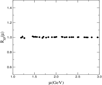
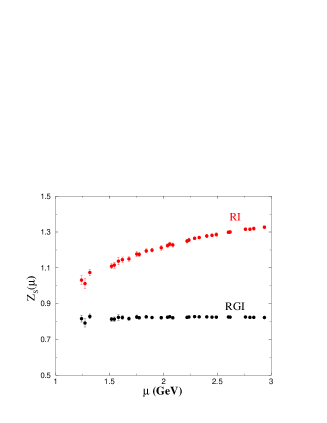
Figure 3: $R_{PS}$ (left) and $Z_{S}(a\mu)$ (right) as a function of the renormalization scale.

4.3 Renormalization of the Scalar Density

To implement the RI/MOM non-perturbative renormalization technique we computed the projected, amputated Green’s functions of the quark bilinears defined in eq. (16). In the first plot of fig. 3 we show the ratio

$$R_{PS}=\frac{(m_{1}-m_{2})\Gamma_{S}\left(p,m_{1},m_{2}\right)}{m_{1}\Gamma_{P}\left(p,m_{1},m_{1}\right)-m_{2}\Gamma_{P}\left(p,m_{2},m_{2}\right)}$$ (33)

for a given combination of masses. As expected from (19) its value is always compatible with one. The ratio of the vector and axial Green’s functions produces analogous results which we do not report here for lack of space. On the other hand the ratio $\Gamma_{P}/\Gamma_{S}$ with degenerate masses is expected to be sensitive to non-perturbative Goldstone pole contributions [19, 13]. A detailed analysis will be presented in a forthcoming paper.

To calculate $Z_{S}$ in the RI/MOM scheme, we computed the ratio [9]

$$R_{AS}(m)=Z_{A}\frac{\Gamma_{A}(p,m)}{\Gamma_{S}(p,m)}$$ (34)

which we extrapolated to the chiral limit as

$$R_{AS}(m)=Z_{S}^{RI}+Am^{2}+Bm^{-2}$$ (35)

to take into account the effect of unsuppressed zero modes. The results we thus obtained, shown in the second plot of fig. 3, lead to

$$Z_{S}^{\mbox{\scriptsize RI}}(2\,\mbox{GeV})=1.24(5)$$ (36)

where the error is mainly systematics and is due to the uncertainty in the value of the renormalization scale and to the chiral extrapolation (the latter estimated by using different forms of the extrapolating function). Using known results from NNLO continuum perturbation theory[15], we convert eq. (36) to the $\overline{\mbox{MS}}$ scheme, obtaining

$$Z_{S}^{\overline{\mbox{\scriptsize MS}}}(2\mbox{GeV})=1.41(6)$$ (37)

This result is in good agreement with the one in [20] which was determined by fixing the renormalized quark mass value. Invoking again NNLO continuum perturbation theory, we calculate $Z_{S}^{RGI}$ from eq. (18). We use $N_{f}=0$ and $\Lambda_{QCD}=0.238(19)$ [21]. The result, displayed in the second plot of fig. 3 shows the remarkable flatness of $Z_{S}^{RGI}$ for $\mu>1.5$ GeV which confirms the high level of improvement reached by the overlap regularization. Averaging over the region $(1.5-3)$ GeV, we find

$$Z_{S}^{RGI}=0.82(3)$$ (38)

5 Physical Results

In this section we will use our lattice results to infer the renormalized values of the sum of the strange and average up-down quark masses and of the chiral condensate. From eq. (26) we obtain

$$m_{s}(a)+\hat{m}(a)=149(9)\,\mbox{MeV}$$ (39)

where the error is statistical only. Since our volume is fairly large, we expect our main sources of systematic errors to come from discretization effects and from the quenched approximation. For a rough estimate of the systematic error due to quenching approximation we can use the results in [22], from which one sees that, within the quenched approximation, the use of alternative observables to calculate the lattice spacing can produce differences of approximately $10\%$. Had we used $r_{0}$ [23] to fix our lattice spacing we would have obtained a number $\sim 7\%$ higher than the one in eq. (39). Combining this fact with the results in [24], we infer that discretization uncertainties are below $10\%$. If we had used the experimental NNLO results from $\alpha_{s}(M_{Z})=0.118$ in the matching of the renormalization constants in eq. (37), we would have obtained a value of the scalar renormalization constant $\sim 10\%$ higher than the one given above. The difference can be taken as an indication of the systematic error introduced by the quenched approximation. In order to be conservative, we will take $15\%$ as the estimate of our overall systematic error in the renormalized quark masses due to quenching and discretization effects. A more precise estimate of the systematic errors will need much more extensive simulations, which would go beyond the capability of our current computer resources and the exploratory nature of the our work. Combining the results in eqs. (36) and (39) we obtain

$$(m_{s}+\hat{m})^{\mbox{\scriptsize RI}}(\mbox{2 GeV})=120\pm 7\pm 21\,\mbox{MeV}$$ (40)

which represent one of the main results of this work. By using the quark mass ratio $m_{s}/\hat{m}=24.4\pm 1.5$ from chiral perturbation theory [25] the above translates to

$$m_{s}^{\overline{\mbox{\scriptsize MS}}}(\mbox{2 GeV})=102\pm 6\pm 18\,\mbox{MeV}$$ (41)

This result agrees very well with the current lattice world average [26].

Insofar as the value of the condensate is concerned, if we used the standard two-step approach, i.e. first measure the dimensionless condensate, see eqs. (28) or (29), and then multiply it by the cubic power of the lattice spacing, the result would be affected by a very large systematic error due to the uncertainty in the determination of the lattice spacing in quenched simulations. Instead, we will use an alternative method [27]. We write the GMOR relation (12) for the renormalized condensate as follows

$$\chi(a)=-{\displaystyle{1\over 4}}f_{\chi}^{2}{\cal B}_{M_{P}}a^{-1}$$ (42)

where ${\cal B}_{M_{P}}$ is defined in eq. (25) and $f_{\chi}=0.1282$ GeV is the “experimental” value, in physical units, of the pseudoscalar decay constant extrapolated to the chiral limit. While computing the condensate from the above formula relies on an additional element of experimental information, it has several advantages. The most important is that, by expressing the condensate in terms of $f_{\chi}$, we are left with only one power of the UV cutoff $a^{-1}$. With this method we obtain

$$\langle\bar{\psi}\psi\rangle^{\mbox{\scriptsize RI}}(\mbox{2 GeV})=$$ (43)

$$-\,0.0167\pm 0.0010\pm 0.0029\,\mbox{GeV}^{3}$$

where the estimate of the systematic error has been made using the same criteria we used to compute the error for the quark masses. This is our best value for the chiral condensate. It is interesting to note that, if we had used the standard technique, starting from eq. (28), we would have obtained a result with a central value very close to the value in eq. (43), but with a much higher error. Finally, from eq. (43) and NNLO matching, we get

$$\langle\bar{\psi}\psi\rangle^{\overline{\mbox{\scriptsize MS}}}(\mbox{2 GeV})=-\,\left(267\pm 5\pm 15\,\mbox{MeV}\right)^{3}$$ (44)

This result is in very good agreement with the result obtained by the authors of refs. [28, 29], while it is smaller than the result in [30], even if still compatible within errors. Our result is also compatible within errors with the number obtained few years ago in [27] with Wilson-type fermions. We expect, though, the systematics due to the discretization effects to be smaller (${\cal O}(a^{2})$) in the result reported in eq. (44) than the error (${\cal O}(a)$) which affects the determination in [27].

6 Conclusions

At this conference we presented results for the pseudoscalar meson masses and decay constants together with the first fully non-perturbative computation of $(m_{s}+\hat{m})$ with overlap fermions in the quenched approximation. We also computed the chiral condensate $\langle\bar{\psi}\psi\rangle$ from the GMOR relation and directly. To avoid uncertainties due to lattice perturbation theory, we computed the multiplicative renormalization constant $Z_{S}(\mu a)$ non-perturbatively in the RI/MOM scheme. While the systematics errors due to quenching are common to previous calculations, the other systematic errors (mostly discretization effects) are different than in other lattice regularizations and likely to be smaller, because of chiral symmetry. Our results have indeed produced a remarkable verification of “good chiral behavior” of the overlap fermions both in the axial Ward identity and for the pseudoscalar masses.

The calculation of light quark masses uses many of the ingredients needed for a lattice calculation of weak matrix elements, although the latter is computationally more demanding. From this point of view, the very good agreement between our results for the quark masses and the current lattice world average bodes well for the use of the overlap formalism also in matrix element calculations. Our investigation has been mostly of exploratory nature. One would need to extend it to larger volumes and better statistics. Nevertheless, we believe that it demonstrated that the overlap formalism can be used effectively, with known algorithms and the present generation of computers, for large scale QCD calculations, at least in the quenched approximation. Thus we would conclude that it represents a very promising non-perturbative regularization for solving long standing problems, such as the proof of the $\Delta I=1/2$ rule and the calculation of $\epsilon^{\prime}/\epsilon$.

Appendix A Implementation of the Overlap Operator

The complicated form of Neuberger operator renders its numerical implementation more involved and expensive than those of the most common regularizations. The crucial point is to implement the sign function

$$\epsilon(H)=\mbox{sign}(H)$$ (45)

over the whole spectrum of eigenvalues of $H=\gamma_{5}X$. Exact diagonalization is feasible [31] for two dimensional models, but becomes prohibitive for larger systems such as QCD. Many algorithms have been proposed in the literature [32, 33, 34]. We opted for the optimal rational function approximation suggested in refs. [32, 34]. Starting from the observation [32] that the sign function can be written as

$$\varepsilon(x) = \lim_{N\rightarrow\infty}\varepsilon_{N}(x)$$

$$\varepsilon_{N}(x) = x\left(c_{0}+\sum_{k=1}^{N}\frac{c_{k}}{x^{2}+q_{k}}\right)$$ (46)

a good approximation can be obtained at finite $N$ by fixing the coefficients $c_{k}$ and $q_{k}$ with the Remez algorithm [34, 35].

The numerical procedure we have followed to obtain a quark propagator from a fixed source vector $|\eta\rangle$, i.e. solving the equation

$$\left[(1-\frac{1}{2\rho}m_{i})D+m_{i}\right]|\chi_{i}\rangle=|\eta\rangle$$ (47)

is the following:

• We have extracted the $15$ smallest eigenvalues of $H^{2}$ and the corresponding eigenvectors minimizing the Ritz functional [36], projected them out and treated the action of $\epsilon(H)$ on this subspace exactly. The minimum precision required for each eigenvalue $\lambda^{2}_{i}$ is

  $$r_{ritz}\equiv\sqrt{\frac{|H^{2}|\lambda_{i}\rangle-\lambda^{2}_{i}|\lambda_{i}\rangle|^{2}}{\langle\lambda_{i}|\lambda_{i}\rangle}}<10^{-6}$$ (48)

  where $|\lambda_{i}\rangle$ is the corresponding eigenvector. We checked on all the configurations that the largest eigenvalue extracted is always $|\lambda_{max}|>0.15$.

• We have rescaled the reduced matrix $\tilde{H}=H/r$ by a factor $r=3.7$ and we have approximated $\epsilon(\tilde{H})$ as in eq. (46) with $N=14$ and $c_{k},q_{k}$ fixed with the Remez algorithm [34, 35] which guarantees a precision

  $$|\epsilon(\tilde{H})-\epsilon_{N}(\tilde{H})|\leq 3.6\times 10^{-6}$$ (49)

  in the range $\tilde{H}\in[0.040,1.8]$. In order to invert all the equations

  $$\left(\tilde{H}^{2}+q_{k}\right)|\psi_{k}\rangle=|s\rangle\qquad N=1,\dots 14$$ (50)

  in one stroke we use an (inner) multi conjugate gradient (MCG) solver [37]. Note, that during the inner MCG it is necessary to store only $N+2$ large vectors since we are only interested in

  $$|\psi\rangle=\sum_{k=1}^{N}c_{k}|\psi_{k}\rangle\$$ (51)

  The convergence is governed by the inversion corresponding to the smallest $q_{k}$ for which we require a residual

  $$r_{in}\equiv\sqrt{\frac{|(\tilde{H}^{2}+q_{14})|\psi_{14}\rangle-|s\rangle|^{2}}{\langle s|s\rangle}}<10^{-6}$$ (52)

  Notice that having extracted the lowest eigenvectors of $H^{2}$ improves the approximation used for $\varepsilon(H)$ and reduces the condition number of $H^{2}$, which results in a speed up of the inversion in eq. (50).

• From eq. (47) and using the GWR we can write

  $$|\chi_{i}\rangle=\frac{\rho\left((1-\frac{m_{i}}{2\rho})D^{\dagger}+m_{i}\right)}{\left(\rho^{2}-m_{i}^{2}/4\right)\left(D+D^{\dagger}\right)+\rho m_{i}^{2}}|\eta\rangle$$ (53)

  and therefore we are left to invert

  $$\left(D+D^{\dagger}+\frac{\rho m_{i}^{2}}{\rho^{2}-m_{i}^{2}/4}\right)|\tilde{\chi}_{i}\rangle=|\eta\rangle$$ (54)

  $D+D^{\dagger}$ is an Hermitian matrix and therefore a MCG can be applied also in this case. Moreover $[D+D^{+},\gamma_{5}]=0$ implies that we can always use sources $|\eta\rangle$ and solutions $|\chi_{i}\rangle$ restricted to one chiral sector, saving one application of $\varepsilon(H)$ per iteration [34]. The convergence is governed by the inversion corresponding to the smallest quark mass, for which we require a residual of $r_{out}<10^{-5}$

We did not attempt to use any preconditioning for the inner and the outer MCG. At the $i$-th step of the outer MCG, the difference $|d_{i}\rangle$ of two consecutive source vectors $|s_{i}\rangle$ and $|s_{i-1}\rangle$ on which $\varepsilon_{N}(H)$ has to be applied gets smaller and smaller when $r_{out}$ decreases. Therefore at the $i+1$ step we have applied $\varepsilon_{N}(H)$ directly on $|d_{i}\rangle$ with an increased $r_{in}$ (every $40$ outer MCG step we required always the full precision to avoid rounding accumulation). After convergence, we always checked that the true residual associated with the eq. (47) for each mass is $<10^{-5}$. In our simulations the average numbers of inner and outer iterations is ${\cal O}(150)$ and ${\cal O}(250)$ respectively.

References

- [1] D. B. Kaplan, Phys. Lett. B288 (1992) 342.
- [2] R. Narayanan, H. Neuberger, Phys. Lett. B302 (1993) 62, Nucl. Phys. B443 (1995) 305.
- [3] H. Neuberger, Phys. Lett. B417 (1998) 141, Phys. Lett. B427 (1998) 353.
- [4] P. H. Ginsparg, K. G. Wilson, Phys. Rev. D25 (1982) 2649.
- [5] M. Lüscher, Phys. Lett. B428 (1998) 342.
-
[6]
H. Neuberger,
Nucl. Phys. (Proc. Suppl.) 83 (2000) 67;
P. Hernandez, these proceedings;
Y. Kikukawa, these proceedings;
P. Hasenfratz, these proceedings. - [7] S. Capitani, L. Giusti, Phys. Rev. D62 (2000) 114506, Phys. Rev. D64 (2001) 014506.
- [8] V. Gimenez, L. Giusti, F. Rapuano, M. Talevi, Nucl. Phys. B540 (1999) 472.
- [9] L. Giusti, C. Hoelbling, C. Rebbi, hep-lat/0108007 and in preparation.
- [10] C. Alexandrou, E. Follana, H. Panagopoulos, E. Vicari, Nucl. Phys. B580 (2000) 394.
- [11] P. Hasenfratz, Nucl. Phys. B525 (1998) 401.
- [12] Y. Kikukawa, A. Yamada, Nucl. Phys. B547 (1999) 413.
- [13] G. Martinelli et al., Nucl. Phys. B445 (1995) 81.
- [14] L. Giusti, A. Vladikas, Phys. Lett. B488 (2000) 303.
- [15] V. Gimenez, L. Giusti, F. Rapuano, M. Talevi, Nucl. Phys. B531 (1998) 429.
- [16] G. Kilcup, D. Pekurovsky, L. Venkataraman, Nucl. Phys. (Proc. Suppl.) 53 (1997) 345. Repository at the “Gauge Connection” (http://qcd.nersc.gov/).
- [17] T. Blum et al., hep-lat/0007038.
- [18] C. R. Allton, V. Gimenez, L. Giusti, F. Rapuano, Nucl. Phys. B489 (1997) 427.
-
[19]
H.D. Politzer, Nucl.Phys. B117 (1976) 397;
P. Pasqual, E. de Rafael, Z. Phys. C12 (1982) 127. - [20] H. Wittig, these proceedings.
- [21] S. Capitani, M. Luscher, R. Sommer, H. Wittig, Nucl. Phys. B544 (1999) 669.
- [22] S. Aoki et al., Phys. Rev. D60 (1999) 114508.
- [23] M. Guagnelli, R. Sommer, H. Wittig, Nucl. Phys. B535 (1998) 389.
- [24] J. Garden, J. Heitger, R. Sommer, H. Wittig, Nucl. Phys. B571 (2000) 237.
- [25] H. Leutwyler, Phys. Lett. B378 (1996) 313.
-
[26]
V. Lubicz,
Nucl. Phys. (Proc. Suppl.) 94 (2001) 116;
T. Kaneko, these proceedings. - [27] L. Giusti, F. Rapuano, M. Talevi A. Vladikas, Nucl. Phys. B538 (1999) 249.
- [28] P. Hernandez, K. Jansen, L. Lellouch H. Wittig, JHEP 0107 (2001) 018.
- [29] P. Hasenfratz et al., hep-lat/0109007.
- [30] T. DeGrand, Phys. Rev. D63 (2001) 034503.
- [31] L. Giusti, C. Hoelbling, C. Rebbi, hep-lat/0101015 and references therein.
- [32] H. Neuberger, Phys. Rev. Lett. 81 (1998) 4060.
- [33] P. Hernandez, K. Jansen, M. Luscher, Nucl. Phys. B552 (1999) 363.
- [34] R. G. Edwards, U. M. Heller, R. Narayanan, Nucl. Phys. B540 (1999) 457. R. G. Edwards, U. M. Heller, R. Narayanan, Phys. Rev. D59 (1999) 094510.
- [35] E. Ya. Remez, General Computational Methods of Chebyshev Approximations. The Problems of Linear Real Parameters.
- [36] T. Kalkreuter, H. Simma, Comput. Phys. Commun. 93 (1996) 33.
- [37] B. Jegerlehner, hep-lat/9612014.