Anisotropic Lattice and Its Application to Quark Gluon Plasma

Abstract

We have studied the link-integration method for the improved actions. With this method the $\eta$ parameter in the medium to strong coupling regions is obtained. Effects of the self-energy terms for the $\eta$ parameters are small in the regions of $\beta$ and $\eta$ studied. After these investigations, the anisotropic lattice is used for the calculation of transport coefficients of the quark gluon plasma.

1 Link Integration For Improved Action

If $R$ is an external source field for link variable $U$, the expectation value of $U$ is given by,

$$<U>=\frac{1}{Z}\frac{dZ(R)}{dR^{\dagger}}$$ (1)

$Z(R)$ is expressed by the modified Bessel function $I_{1}$[1],[2].

$$Z(R)=\oint\frac{dx}{2\pi i}e^{xQ}\frac{1}{z}I_{1}(2z)$$ (2)

where

$$z=\left(\frac{P(x)}{x}\right)^{\frac{1}{2}}$$

$$Q=2Re(det(R))$$

$$\begin{array}[]{ll}P(x)=1+xTr(RR^{\dagger})\\ \hskip 28.45274pt+\frac{1}{2}x^{2}\left[(Tr(RR^{\dagger}))^{2}-Tr((RR^{\dagger})^{2})\right]\\ \hskip 28.45274pt+x^{3}det(RR^{\dagger})\end{array}$$ (3)

Similarly $dZ(R)/dR$ is written by the $I_{1}$ and $I_{2}$[1],[2].
The path of the integration is a closed circle on the complex plane $x$. In principle its radius $r$ is arbitrary, but numerical integration requires adequate radius. We apply Simpson method for the numerical integration, and search for the region of $r$ and number of the division $N$ where $<U>$ is stable with the change of $r$ and $N$. It is observed that the $<U>$ depends strongly on $r$ and $N$. For example if we take $N=50$, there appear spurious plateaus, which disappears with increasing $N$. However there is a region of $r$ in which $<U>$ is stable for the change of $r$ and $N$. It becomes a little wider as $N$ is increased. This region of $r$ is called an optimal region of integration;$r^{opt}$. The link integration should be done with $r^{opt}$
The $r^{opt}$ are shown as a function of $\beta$ in Fig.1.

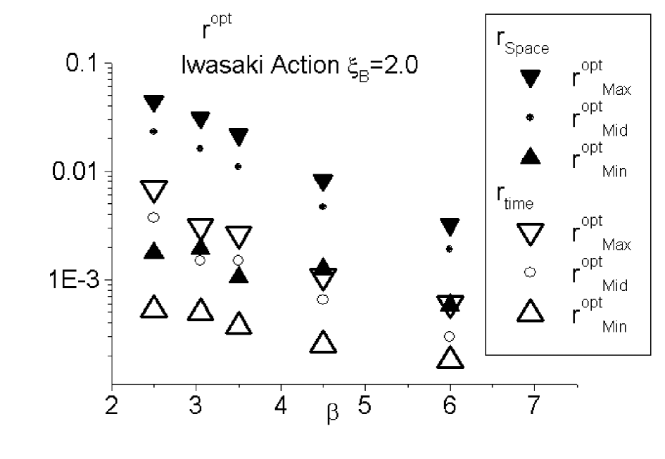
Figure 1: An example of $r^{opt}_{max}$, $r^{opt}_{min}$ and $r^{opt}_{mid}$ on a fully thermalized configuration

Notice that $r^{opt}$ region changes with the position of link variables on a configuration and also with configurations due to the fluctuation of gauge fields. The results shown in Fig.1 are not the average over the fluctuations. But the fluctuation of the $r^{opt}$ region is not large. If we choose,

$$r^{opt}\sim r^{opt}_{mid}=\displaystyle{\frac{r^{opt}_{max}+r^{opt}_{min}}{2}}$$ (4)

it has been in an optimal region of $r$ throughout the link variables and configurations. The $r^{opt}$ for space link $U_{space}$ is larger than that of $U_{time}$ when $\xi>1$; $r^{opt}_{space}>r^{opt}_{time}$, and they become smaller for larger $\beta$.

In the case of improved actions, the number of link $U$ which are simultaneously integrated in a loop becomes much smaller than the case of standard action. Therefore the link integration method is not effective for the calculation of smaller Wilson loops. The suppression of the fluctuation is impressive for $W(6\times 6)$ but not for $W(4\times 4)$ for $\beta=2.5$. However for the calculation of $\eta$ in the smaller $\beta$ region, the use of the link integration method has been indispensable. We have used it for the calculation of $\eta$ at $\beta=3.5,3.05,2.5$ for Iwasaki action.

2 Self-energy Effects on $\eta$

Lattice potential is defined by the ratio of Wilson loops, $V(r)=log(\displaystyle{\frac{W(p,r)}{W(p+1,r)}})$. The $\xi_{R}$ is determined by the matching of the potential in space and temporal direction.

$$V_{s}(\xi_{B},r)=V_{t}(\xi_{B},t=\xi_{R}\times r)$$ (5)

The $\eta$ parameter is defined by $\eta=\xi_{R}/\xi_{B}$ However, $V_{s}$ and $V_{t}$ includes self-energy contributions which may be written as,

$$V_{s}(\xi_{B},r)=V_{s}^{0}(\xi_{B})+V_{s}(\xi_{B},r)$$ (6)

Similarly for $V_{t}(\xi_{B},t)$.
Due to the anisotropy, $V_{s}^{0}(\xi_{B})\neq V_{t}^{0}(\xi_{B})$.
For the standard action, the effect of the self-energy term on $\eta$ has been studied by Bielefeld group[4]. It is reported that the effect on $\eta$ is $\sim 0.01$. In this report we study its effects for Iwasaki’s improved action[3]. In order to get rid of the effect of self-energy term $V^{0}$, we employ a subtraction method,

$$V_{s}^{Sub}(\xi_{B},r)=V_{s}(\xi_{B},r)-V_{s}(\xi_{B},r_{0})$$ (7)

similarly for $V_{t}^{Sub}$. The $t_{0}$ and $r_{0}$ should satisfy $t_{0}=\xi_{R}r_{0}$ and we take $r_{0}=3$. Then we apply the matching for $V^{Sub}$[5].

$$V_{s}^{Sub}(\xi_{B},r)=V_{t}^{Sub}(\xi_{B},t=\xi_{R}\times r)$$ (8)

We denote the $\eta$ determined in this way as $\eta^{Sub}$.

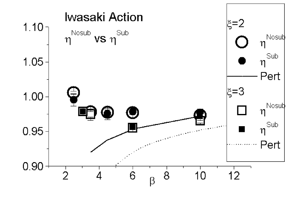
Figure 2: $\eta^{Sub}$(filled circle) and $\eta^{Nosub}$ without subtraction(open Symbols) at $\xi_{R}=2.0$

In Fig.2 we have shown our results. It is found that the differences of the $\eta^{Nosub}$ and $\eta^{Sub}$ are small; $\leq 0.015$.
Combined with the results of Bielefeld group for the standard action, we conclude that the correction to the global dependences of the $\eta$ parameters for the class of improved actions(Symanzik, Iwasaki etc) which we have presented at lattice 99[6] is really small

3 Quark Gluon Plasma on Anisotropic Lattice

As applications of the anisotropic lattice, we have started a simulation of transport coefficients of the quark gluon plasma and a study of the heavy quark spectroscopy[7].

We reported the transport coefficients from lattice simulations on isotropic lattice[8][9]. Our results have been impressive and encouraging for the phenomenological study of the quark gluon plasma, in the sense that they are located close to the simple extrapolation of the perturbative results on the figure at high temperature limit. However they depend on the ansatz for the spectral function of the Matsubara green function($G_{\mu\nu}$) of energy momentum tensor. The aim of this work is to improve the resolution of the $G_{\mu\nu}$ by using the anisotropic lattice, and check the ansatz of the spectral function.
The calculation of the transport coefficients of quark gluon plasma are formulated in the linear response theory. They are calculated by the $G_{\mu\nu}$ of energy momentum tensor. For the pure gauge models it is written as, $T_{\mu\nu}=2\,\mbox{Tr}\,[F_{\mu\sigma}F_{\nu\sigma}-\frac{1}{4}\delta_{\mu\nu}F_{\rho\sigma}F_{\rho\sigma}]$ On an anisotropic lattice, the field strength tensors are written as follows,

$$a_{\sigma}^{3}F_{ij}^{c}F_{ij}^{c}=\frac{\beta_{\xi}}{6a_{\sigma}}\eta(3-TrU_{ij})$$ (9)

$$a_{\sigma}^{3}F_{i4}^{c}F_{i4}^{c}=\frac{\beta_{\xi}}{6a_{\sigma}}\xi_{B}^{2}\eta(3-TrU_{i4})$$ (10)

We have started from test run of calculating $G_{\mu\nu}$ on $8^{3}\times 8$ lattice with Iwasaki action at $\beta=3.3$ and $\xi_{R}=2.0$. As a check of our calculations on the anisotropic lattice, we have compared it with the one from an isotropic lattice $8^{3}\times 4$, for which the scale in temperature direction is changed to $\xi_{R}=2$ lattice. They are shown in Fig.3.

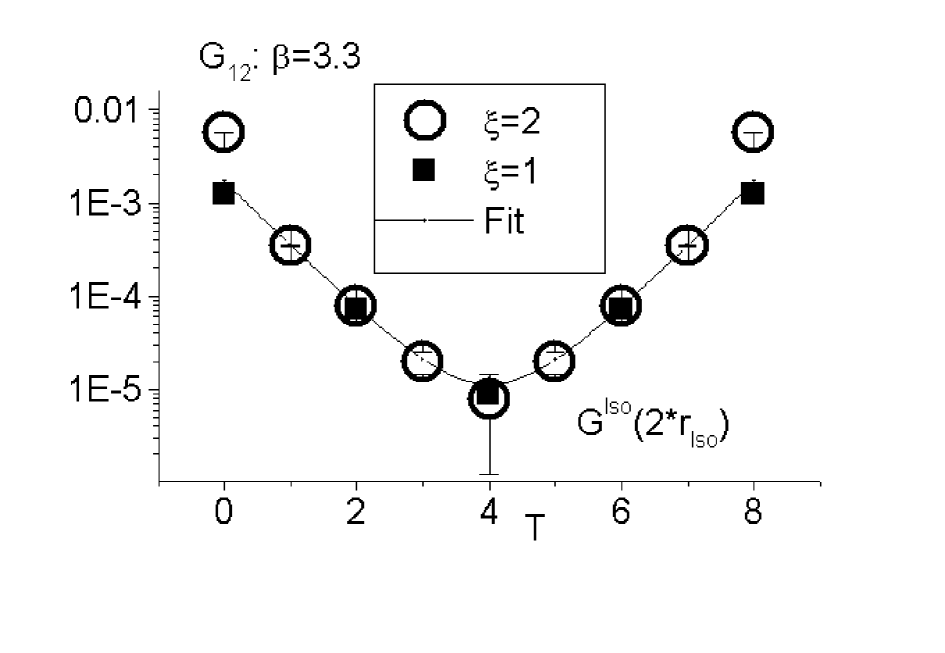
Figure 3: Matsubara green function $G_{12}$ on $8^{3}\times 8$ lattice with $\xi_{B}=2.0$(open circle), and on isotropic $8^{3}\times 4$ lattice(filled square) at $\beta=3.3$

It is seen that the both green functions coincide with each other. The merit of applying an anisotropic lattice is that we could determine the transport coefficients under the ansatz of the spectral function on small lattices.

$$\begin{array}[]{ll}\rho(\vec{p}=0,\omega)\\ \hskip 28.45274pt=\frac{A}{\pi}(\frac{\gamma}{(m-\omega)^{2}+\gamma^{2}}-\frac{\gamma}{(m+\omega)^{2}+\gamma^{2}})\end{array}$$ (11)

Because 3 independent parameters are determined by the 3 independent data points of $G_{12}$ on an anisotropic lattice.
We have proceeded to the calculation of Matsubara green function on $24^{3}\times 16$ lattice with $\xi_{R}=2.0$. At this point, the number of data is not large enough to determine the $G_{\mu\nu}$. But we expect that the check of the ansatz given by Eq.11, could be done on the anisotropic lattice. In addition we are planing to determine spectral functions by the maximum entropy method. They will be reported in the forthcoming publications

ACKNOWLEDGMENTS
This work has been done with SX-5 at RCNP and VX-4 at Yamagata University. We are grateful for the members of RCNP for kind supports.

References

- [1] R.Brower, P.Rossi,and C.I.Tan, Nucl.Phys.B190[FS3](1981) 699
- [2] Ph. deForcrand and C. Roiesnel, Phys. Letters B31(1985),77
- [3] Y. Iwasaki, Nucl. Phys. B258(1985), 141; Univ. of Tsukuba preprint UTHEP-118(1983)
- [4] J.Engels,F.Karsch and T.Scheideler,Nucl.Phys.B564(2000) 303.
- [5] T.R.Klassen hep-lat/9803010
- [6] S.Sakai, A.Nakamura,T.Saito Nucl. Phys.B(Proc Suppl) 83-84(1998), 399
- [7] T.Saito,A.Nakamura and S.Sakai,In this proceedings
- [8] A.Nakamura,T.Saito and S.Sakai, Nucl. Phys.B(Proc Suppl)63(1998),424
- [9] S.Sakai, A. Nakamura and T. Saito Nucl. Phys.A638(1998) 535c-538c