Anisotropic Lattices and Dynamical Fermions

Abstract

We report results from full QCD calculations with two flavors of dynamical staggered fermions on anisotropic lattices. The physical anisotropy as determined from spatial and temporal masses, their corresponding dispersion relations, and spatial and temporal Wilson loops is studied as a function of the bare gauge anisotropy and the bare velocity of light appearing in the Dirac operator. The anisotropy dependence of staggered fermion flavor symmetry breaking is also examined. These results will then be applied to the study of 2-flavor QCD thermodynamics.

1 INTRODUCTION

Anisotropic lattices have been used extensively for $T=0$ calculations[1]. Finite temperature calculations using anisotropic lattices exploit the natural asymmetry of finite temperature field theory to reduce lattice spacing errors associated with the transfer matrix at less cost than is required for the full continuum limit[2].

With a sufficiently small value for the temporal lattice spacing, $a_{t}$, we can vary the temperature in small discrete steps by varying the number of time slices, $N_{t}$. In this study we sweep through the transition by studying different $N_{t}$’s (8–64). Varying the temperature at fixed temporal and spatial lattice spacing separates temperature and lattice spacing effects, allowing a study of the temperature dependence with all other parameters fixed.

The coefficients needed to relate lattice observables to the physical energy and pressure are determined as a by-product of the zero temperature studies needed to choose the bare parameters. Once determined, these “Karsch” coefficients[3] can be used for all temperatures since they depend only on the intrinsic lattice parameters and not on $N_{t}$. This allows a straight-forward determination of the temperature dependence of the energy and pressure, again at fixed lattice spacing. With two or more slightly different values for $a_{t}$, a high-resolution sampling of temperatures can be investigated.

As the temporal lattice spacing, $a_{t}$, approaches the continuum limit $(a_{t}\rightarrow 0)$, the part of the flavor symmetry, which is violated by terms of ${\cal O}(a_{t}^{2})$, is expected to be restored. In this study we are examining our data for evidence of improvement of the flavor symmetry, when $a_{t}$ becomes sufficiently small.

2 THE ANISOTROPIC STAGGERED ACTION

We are simulating full QCD with two dynamical flavors of staggered fermions on an anisotropic lattice. Our calculations are based on the QCD action $S^{\xi}=S_{G}^{\xi}+S_{F}^{\xi}$, where the gauge action is:

$$S_{G}^{\xi}=-\frac{\beta}{N_{c}}\frac{1}{\xi_{o}}\left[\sum_{x,s>s^{\prime}}P_{ss^{\prime}}(x)+\xi_{o}^{2}\sum_{x,s}P_{st}(x)\right],$$

and the fermion action is:

$$S_{F}^{\xi} = \sum_{x}\overline{\psi}(x)\left[m_{f}+\nu_{t}\mathchoice{\ooalign{$\hfil\displaystyle\mkern 1.0mu/\hfil$\crcr$\displaystyle D$}}{\ooalign{$\hfil\textstyle\mkern 1.0mu/\hfil$\crcr$\textstyle D$}}{\ooalign{$\hfil\scriptstyle\mkern 1.0mu/\hfil$\crcr$\scriptstyle D$}}{\ooalign{$\hfil\scriptscriptstyle\mkern 1.0mu/\hfil$\crcr$\scriptscriptstyle D$}}^{\rm Staggered}_{t}\right]\psi(x)$$ (18)

$$+\sum_{x}\overline{\psi}(x)\left[\frac{1}{\xi_{0}}\sum_{s}\mathchoice{\ooalign{$\hfil\displaystyle\mkern 1.0mu/\hfil$\crcr$\displaystyle D$}}{\ooalign{$\hfil\textstyle\mkern 1.0mu/\hfil$\crcr$\textstyle D$}}{\ooalign{$\hfil\scriptstyle\mkern 1.0mu/\hfil$\crcr$\scriptstyle D$}}{\ooalign{$\hfil\scriptscriptstyle\mkern 1.0mu/\hfil$\crcr$\scriptscriptstyle D$}}^{\rm Staggered}_{s}\right]\psi(x).$$

In our simulations we attempt to examine the QCD phase transition for volumes ($16^{3}\times 4$), quark masses ($m_{\pi}/m_{\rho}\approx 0.3$) and a spatial lattice spacing ($a_{s}\approx 0.3$ fm) similar to those used in $N_{t}=4$, 2-flavor thermodynamic studies on isotropic lattices. Thus, we adjust the bare bare anisotropy ($\xi_{0}$) and the renormalization of the speed of light ($\nu_{t}$) to yield the required $a_{s}$ and $m_{\pi}/m_{\rho}$ but work with a much smaller temporal lattice spacing choosen so the critical value of $N_{t}$ is approximately 16.

3 SIMULATIONS

run	volume	traj.	$\beta$	$\xi_{0}$	$m_{f}$
1	$16^{3}$x32	5800	5.425	1.5	0.025
2	$16^{2}$x24x32	5100	5.425	1.5	0.025
3	$16^{2}$x24x64	1300	5.695	2.5	0.025
4	$16^{2}$x24x64	1400	5.725	3.44	0.025
5	$16^{2}$x24x64	3400	5.6	3.75	0.025
6	$16^{2}$x24x64	3200	5.3	3.0	0.008
7	$16^{3}$x24	3500	5.3	3.0	0.008
8	$16^{3}$x20	2800	5.3	3.0	0.008
9	$16^{3}$x16	4500	5.3	3.0	0.008
10	$16^{3}$x12	8200	5.3	3.0	0.008
11	$16^{3}$x8	5500	5.3	3.0	0.008

Table 1: Parameters of all the calculations. All runs have dynamical $\nu_{t}=1.0$ except run 3 which has $\nu_{t}=1.2$.

We have used the zero temperature runs 1-6 for scale-setting and determination of the anisotropy. For all the zero-temperature runs the renormalized anisotropy $\xi_{r}$ is calculated both from the $\rho$ masses in the spatial and temporal directions and from matching the static potentials[4]. Figure 1 shows that both methods provide values for $\xi_{r}$ which are reasonably close.

The idea behind run 7 through 11 is that we keep the spatial lattice spacing, $a_{s}$, and all other run parameters constant and change only the number of lattice points, $N_{t}$, in the temporal direction.

Our simulations implement the R-algorithm[5] with step–size $\Delta t=0.005$ for all jobs from Table 1. Figure 2 shows that our choice of $\Delta t$ is consistent with the requirements for small finite step–size error on the physical quantities.

4 THE VELOCITY OF LIGHT

The velocity of light on a lattice can be defined through the meson dispersion relation:

$$E_{t,phys}^{2}(p_{s}) = \frac{E_{t,lat}^{2}(0)}{a_{t}^{2}}+c_{ts}^{2}(p_{s})P^{2}_{s,lat}\frac{1}{a_{s}^{2}}$$

We tune $\nu_{t}$, so that $c_{ts}(p_{s})\approx 1$. The velocity of light is calculated for the $\pi$ propagating in the temporal direction and having non–zero momentum for three values of $\nu_{t}$: 1.0, 0.8 and 1.2, where the first is a dynamical parameter and the last two are valence parameters. From Figure 3 we see that the choice of $\nu_{t}=1.0$ gives velocity of light closest to 1.0.

5 IMPROVEMENT OF THE FLAVOR SYMMETRY

Table 2 shows the meson masses for run 3 ($a_{s}=0.231(7)$ fm, $a_{t}=0.072(4)$ fm) and run 4 ($a_{s}=0.243(3)$ fm, $a_{t}=0.057(2)$ fm).

We choose $\Delta_{\pi}=(m_{\pi_{2}}-m_{\pi})/m_{\rho}$, where $\pi_{2}$ is the second local staggered pion, as a quantitative measure of the flavor symmetry breaking in the spatial (S) and temporal (T) directions. The data shows that in the temporal direction for both runs $\Delta_{\pi}$ is smaller than its value in the spatial direction, which means that we are seeing improvement of the flavor symmetry as $a_{t}$ becomes finer. Especially for run 4, the $\pi$ and $\pi_{2}$ look virtually degenerate.

am	S, #3	T, #3	S, #4	T, #4
$am_{\pi}$	0.680(3)	0.214(2)	0.771(4)	0.181(2)
$am_{\pi_{2}}$	0.759(12)	0.219(2)	0.836(21)	0.181(2)
$am_{\rho}$	0.902(26)	0.283(4)	0.948(13)	0.222(4)
$\Delta_{\pi}$	0.09(1)	0.017(9)	0.07(2)	0.000(2)

Table 2: Meson masses for run 3 and 4.

6 THE PHASE TRANSITION

The thermodynamics runs 7–11 have volume $16^{3}\times N_{t}$, where $N_{t}=$ 8, 12, 16, 20 and 24. The bare parameters are kept constant for all runs 6–11. Figure 4 shows the sweep through the phase transition as we gradually change the temperature by varying only $N_{t}$. We fit our data to a hyperbolic tangent form and determine $T_{c}\approx 160$ MeV from the inflection point.

7 CONCLUSIONS

We have studied the finite temperature QCD phase transition using staggered fermions on an anisotropic lattice with anisotropy of $\approx 4$. This allows us to explore the temperature dependence of the transition with all other parameters fixed. The results are roughly consistent with earlier, isotropic studies, showing a value of the critical temperature of approximately 160 MeV. While this approach naturally reduces finite lattice spacing errors associated with $a_{t}$, we plan to include improvements to the spatial parts of the staggered fermion action so that the ${\cal O}(a_{s}^{2})$ errors are reduced as well.

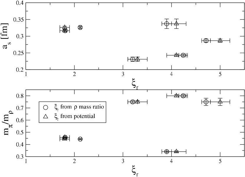
Figure 1: Scatter plots of the zero temperature runs 1–6.

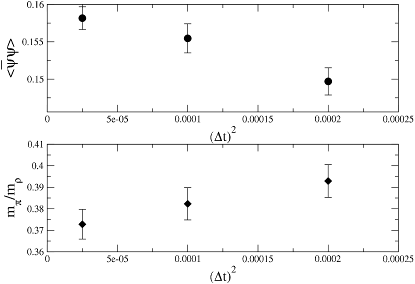
Figure 2: Step–size test. Volume $8^{3}\times 32$, $\beta=5.35$, $\nu_{t}=1.0$, $\xi_{0}=3.5$, $m_{f}=0.006$.

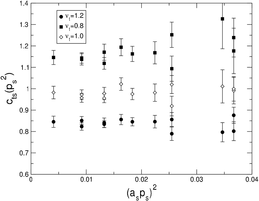
Figure 3: Tuning of the velocity of light using a $16^{2}\times 24\times 64$ volume, $\beta=5.3$, $\xi_{0}=3.0$, $m_{f}=0.008$.

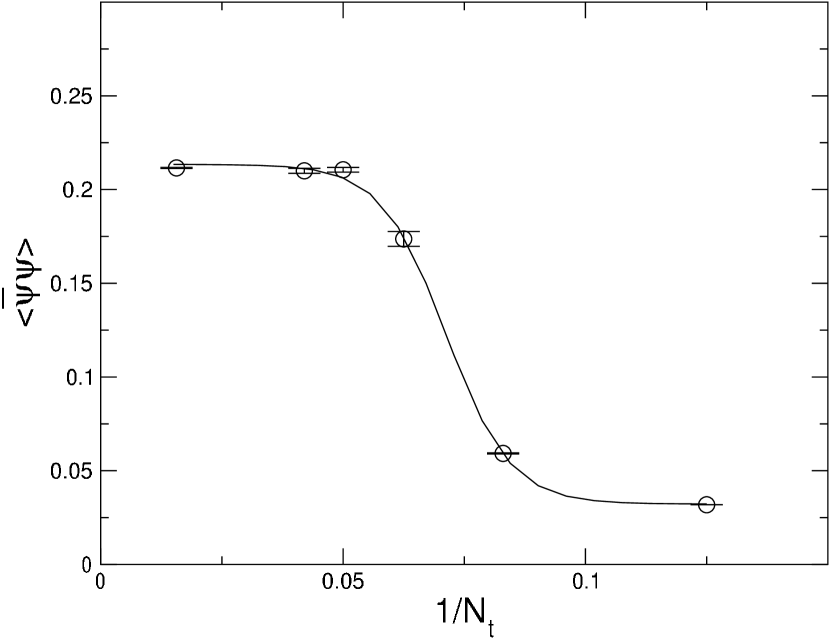
Figure 4: The temperature dependence of $\langle\overline{\psi}\psi\rangle$ in the region of $T_{c}$.

References

- [1] C. Morningstar and M. Peardon, Phys.Rev. D60:034509 (1999)
- [2] QCD-TARO Collaboration: Ph. de Forcrand et al., Phys.Rev.D63:054501 (2001)
- [3] F. Karsch, Nucl.Phys.B205[FS5], 285 (1982)
- [4] T. Klassen, Nucl.Phys.B533, 557 (1998)
- [5] S. Gottlieb et al., Phys.Rev.D35, 2531 (1987)