Extraction of $K\rightarrow\pi\pi$ Matrix Elements with Wilson Fermions

Abstract

We present the status of a lattice calculation for the $K\rightarrow\pi\pi$ matrix elements of the $\Delta S\!\!=\!\!1$ effective weak Hamiltonian, directly with two pion in the final state. We study the energy shift of two pion in a finite volume both in the $I\!\!=\!\!0$ and $I\!\!=\!\!2$ channels. We explain a method to avoid the Goldstone pole contamination in the computation of renormalization constants for $\Delta I\!\!=\!\!3/2$ operators. Finally we show some preliminary results for the matrix elements of $\Delta I\!\!=\!\!1/2$ operators. Our quenched simulation is done at $\beta\!\!=\!\!6.0$, with Wilson fermions, on a $24^{3}\times 64$ lattice.

1 General Strategy

Kaon weak decay amplitudes can be described in terms of matrix elements (ME’s) of the $\Delta S\!\!=\!\!1$ effective weak Hamiltonian. ${\cal H}^{\Delta S=1}$ is written as a linear combination of a complete basis of renormalized local operators (OP’s) $Q_{i}(\mu)$, where $\mu$ is the renormalization scale. The most relevant contributions in the computation of the weak amplitudes ${\cal A}_{I=0,2}$ and of $\epsilon^{\prime}/\epsilon$ are given by the $K\!\!\rightarrow\!\!\pi\pi$ ME’s of $\hat{Q}^{+}$, $\hat{Q}^{-}$, $\hat{Q}_{6}$, $\hat{Q}_{7}$ and $\hat{Q}_{8}$ (see below and Ref. [1, 2]). In order to compute these ME’s from lattice QCD, one has to renormalize the bare (divergent) lattice OP’s. Two methods are possible on the lattice:
$1)$ Compute $\langle 0|\hat{Q}_{i}(\mu)|K\rangle$ and $\langle\pi|\hat{Q}_{i}(\mu)|K\rangle$ and then derive $\langle\pi\pi|\hat{Q}_{i}(\mu)|K\rangle_{I=0,2}$ using soft pion theorems [3]. In this case, besides the difficulties in controlling chiral behaviour, a major problem is the inclusion of higher order contributions in the chiral expansion which should reconstruct the final state interaction (FSI). In fact, in this approach, only $K\rightarrow\pi\pi$ ME’s at lowest order in ChPT can be obtained (see Refs. [4]).
$2)$ Compute directly $\langle\pi\pi|\hat{Q}_{i}(\mu)|K\rangle_{I=0,2}$. The main difficulty in this case is the relation between ME’s in a (Euclidean) finite volume and the corresponding physical infinite volume ones. Even if, in principle, it is possible to take into account FSI exactly [5, 6], in practice these methods are numerically very demanding. So, with present computing power, only simulation at unphysical kinematics [1] may be achieved, and ChPT is still needed to extrapolate to the physical point.

In this work we choose the second strategy. To extract ME’s we place the local OP $Q_{i}$ in the origin and we use three local interpolating fields (e.g. the pseudoscalar density $P^{ab}=\bar{\psi}^{a}\gamma_{5}\psi^{b}$), one at time $t_{2}=10$ which annihilates one $\pi$ in the two pion state and one at time $t_{K}=54\equiv-10$ which creates a $K$ (both with momentum zero). As explained below $t_{2}$ ($t_{K}$) must be chosen large enough in modulus for the two pion state (the kaon state) to be already asymptotic. The third one annihilates at time $t_{1}$ (not fixed) the second $\pi$ with momentum either $0$ or $2\pi/L$. As shown in [6], in the limit $T/2\!>\!t_{1}\!\gg\!t_{2}\!\gg 0$,  $T\!\gg\!t_{K}\!>\!T/2$ we have

$$\hskip 5.69046pt\frac{\langle 0|T[\hat{\pi}_{1}(t_{1})\hat{\pi}_{2}(t_{2})Q_{i}(0)\hat{K}(t_{K})]|0\rangle_{V}}{G_{\pi}(t_{1})G_{\pi}(t_{2})G_{K}(t_{K})}Z_{\pi}^{2}Z_{K}\,\longrightarrow$$

$$\longrightarrow|\langle\pi\pi|Q_{i}|K\rangle|\cos\delta(W)\;\textrm{\large e}^{{}^{-(W-2M_{\pi})t_{2}}}\!\!+O\Big{(}\frac{1}{L}\Big{)}\qquad$$

where $G_{\pi}(t)\!\!=\!\!\langle 0|T[\hat{\pi}(t)\hat{\pi}^{\dagger}(0)]|0\rangle_{V}$, $Z_{\pi}\!\!=\!\!|\langle 0|\hat{\pi}|\pi\rangle|$ (the definition of $G_{K}(t)$ and $Z_{K}$ is analougous), $|\pi\pi\rangle$ is the lower two pion state with the same momentum of $\hat{\pi}_{1}(t_{1})$. $\Delta E=W-2M_{\pi}$ is the energy shift of two pions in a finite volume (FV) while $\delta(W)$ is the strong interaction phase (which depends on the isospin and on the energy of the two pion state). In order to extract the physical ME, one needs to compute FV corrections, which are represented by the correction to the ME (indicated above by the term $O(1/L)$) and by the FV energy shift. We focus now on this last issue. Theoretical predictions [7, 8] show that the factor $\exp(-\Delta Et_{2})$ should give relevant corrections: of order $5\div 10\%$ in the $\Delta I=3/2$ channel and of order $25\%$ (or larger) in the $\Delta I=1/2$ one.

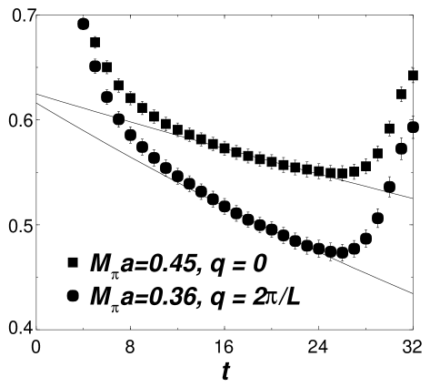
Figure 1: a. $G_{4\pi}(t)/G_{\pi}(t)^{2}$  
               b. effective mass of  $G_{2\pi S}(t)/G_{\pi}(t)^{2}$

2 Finite Volume Energy Shift

To extract $\Delta E$ we study the four point function $G_{4\pi}(t)=\langle 0|T[\hat{\pi}_{4}(t)\hat{\pi}_{3}(t)\hat{\pi}^{\dagger}_{2}(0)\hat{\pi}^{\dagger}_{1}(0)]|0\rangle_{V}$. Since the computation of the $I=0$ correlator require the computation of $T$ $S_{1}$ propagators, we use $G_{4\pi}(t)$ only for $I=2$. We have $\hat{\pi}_{2}(0)\hat{\pi}_{1}(0)=P(0)P(0)$ while $\hat{\pi}_{4}(t)\hat{\pi}_{3}(t)=\sum_{\mbox{\bf{x}}}P(\mbox{\bf{x}},t)\exp{i\mbox{\bf{q}}\mbox{\bf{x}}}\sum_{\mbox{\bf{y}}}P(\mbox{\bf{y}},t)$ with $\mbox{\bf{q}}\!=\!0,2\pi/L$ and with the appropriate flavour structure. Due to the possibility of propagation both of a two pion state in one temporal direction and of a state composed by two single pion states in opposite directions, in the region $T\gg t\gg 0$ one has

$$G_{4\pi}(t)/G_{\pi}(t)^{2}\longrightarrow\frac{C_{\pi\pi}\cosh(W(t-\frac{T}{2}))+C_{\pi}}{\cosh(M_{\pi}(t-\frac{T}{2}))^{2}}$$

where $C_{\pi\pi}$ and $C_{\pi}$ depend on the ME’s of the interpolating fields and on the energy shift. We thus make a fit with $A\exp(-\Delta Et)$ in the region $T/2\gg t\gg 0$ (see Fig. 1.a).

In the $I=0$ channel we use instead $G_{2\pi S}(t)=\langle 0|T[S(t)\hat{\pi}^{\dagger}_{2}(0)\hat{\pi}^{\dagger}_{1}(0)]|0\rangle_{V}$ where $S$ is the scalar density summed over the space and $\hat{\pi}_{2}(0)\hat{\pi}_{1}(0)=\Pi(0)\sum_{\mbox{\bf{x}}}P(\mbox{\bf{x}},0)$, with $\Pi$ equal either to $P$ or to $A_{0}$ (the temporal component of the axial current). We have computed only the connected part, because we expect the disconnected one to be negligible since it is suppressed by the OZI rule. To check this assumption, a computation of the disconnected part is presently under way. We observe empirically that, for $\Pi\!\!=\!\!A_{0}$, the noise is smaller and the plateaux start at smaller times (already $t\!\simeq\!10$ seems sufficients, see Fig. 1.b). Results for both $I\!\!=\!\!2$ and $I\!\!=\!\!0$ channel are shown in Table 1. We compare numerical results both with Lüscher formula [7]

$$\Delta E_{L}\!=\!-\!\frac{4\pi a^{I=0,2}_{0}}{M_{\pi}L^{3}}\!+\!{\cal O}\Big{(}\frac{1}{L^{4}}\Big{)}\;\textrm{with}\;\left\{\begin{array}[]{c}\!a^{I=2}_{0}\!=\!-\frac{M_{\pi}}{8\pi F_{\pi}^{2}}\\ \!a^{I=0}_{0}\!=\!\frac{7M_{\pi}}{16\pi F_{\pi}^{2}}\end{array}\right.$$ (3)

(where $a^{I=0,2}_{0}$ is the tree level result in ChPT) and with its version $\Delta E_{BG}$ in 1-loop quenched ChPT [8] which, in the $I\!=\!0$ case, shows enhanced finite volume correction. For $I\!\!=\!\!2$ there is very good agreement between numerical values and theoretical predictions. For $I\!\!=\!\!0$ there is a striking disagreement for the two heaviest masses while in the lightest case, also due to the large errors, they are compatible. Moreover the dependence with the mass of the pion is different to the one predicted. This could be due to the presence, for large unphysical quark masses, of a stable scalar particle below the two pion state. In this case the behaviour of the shift measured should have only exponentially small correction in the volume. Instead the “genuine” FV energy shift of the two pion state has a power dependence on the volume. To clarify the situation we are thus currently varying the volume of our simulations and trying to reach smaller masses.

$M_{\pi}$	0.446(2)	0.361(2)	0.260(2)
$I=2\qquad 750\;\textrm{conf.}$
$\Delta E^{N}_{\mbox{\bf{q}}=0}$	5.4(6)(5)	6.2(7)(5)	6.6(9)(5)
$\Delta E^{N}_{\mbox{\bf{q}}=\frac{2\pi}{L}}$	8.6(8)(5)	10.9(11)(8)	15.2(27)(8)
$\Delta E_{L}$	4.9(2)	5.6(2)	6.8(3)
$\Delta E_{BG}$	5.3(2)	6.1(2)	7.3(3)
$I=0\qquad 600\;\textrm{conf.}$
$\Delta E^{N}$	-172(10)	-96(11)	-36(21)
$\Delta E_{L}$	-17.1(5)	-19.7(7)	-23.7(11)
$\Delta E_{BG}$	-15.4(4)	-18.0(6)	-22.0(9)

Table 1: Results in lattice units multiplied by $\!10^{3}\!$

3 Renormalization and Goldstone Pole

The renormalization of $\Delta I=3/2$ 4-fermion OP’s, which mix only with OP’s of the same dimension, may be achieved with the method of ref. [9]. This requires the existence of a window $\Lambda_{QCD}\ll\mu\ll 1/a$, where the first inequality serves to avoid pure non-perturbative effects like the coupling to the Goldstone boson. In some cases [10, 11] this makes the chiral limit ill-defined and causes a systematic error in the extrapolation. It is easy to show that for parity conservig OP’s this coupling gives both a single and a double pole, while in the parity violating (PV) case only a single pole is present. For the sake of illustration, we explain the procedure to remove this unwanted contribution only in the PV case. Consider the amputated Fourier transform (at equal external momenta $p$) of the Green functions $G_{i}=\langle\psi(x_{1})\bar{\psi}(x_{2})O_{i}(0)\psi(x_{3})\bar{\psi}(x_{4})\rangle$. By projecting this array onto the possible indipendent Dirac structure we obtain a $5\times 5$ matrix $D(M^{2}_{\pi},p^{2})$ from which the matrix of RC’s is obtained [12] by $Z(\mu a)=Z_{\psi}^{2}(D^{T})^{-1}|_{p^{2}=\mu^{2}}$, where $Z_{\psi}$ is the quark field RC. The pole is present e.g. in $D_{33}$, which corresponds to the OP $O_{3}=SP-PS$. This is evident from Fig. 2.a. To subtract it, it is possible either to fit each element of $D$ directly with $A(p^{2})+B(p^{2})/M^{2}_{\pi}+C(p^{2})M^{2}_{\pi}$ or to construct the combination

Figure 2: a. $D_{33}(M_{\pi}^{2},p^{2})$ b. $(Z(\mu)Z^{{}^{-1}}(\mu_{0})U^{{}^{-1}}(\mu,\mu_{0}))_{{}_{33}}$

$$\qquad\frac{D(M_{1}^{2},p^{2})M_{1}^{2}-D(M_{2}^{2},p^{2})M_{2}^{2}}{M_{1}^{2}-M_{2}^{2}}$$ (4)

(for non-equal masses), which automatically cancels the pole [13], and fit it with $\tilde{A}(p^{2})+\tilde{C}(p^{2})(M^{2}_{1}+M^{2}_{2})$. Finally, by using either $A(p^{2})$ or $\tilde{A}(p^{2})$, we obtain two determination of the RC’s perfectly compatible with each other. In Fig. 2.b the behaviour of $(Z(\mu)Z^{{}^{-1}}(\mu_{0})U^{{}^{-1}}(\mu,\mu_{0}))_{{}_{33}}$ (where $U(\mu,\mu_{0})$ is the renormalization group evolution between $\mu_{0}$ and $\mu$ at NLO) is shown with $\mu_{0}=1.5\;{\rm GeV}$, before and after the subtraction. It is clear that there is a window for $2.4\,{\rm GeV}\geq\mu\geq 1.4\,{\rm GeV}$ where $Z$ follows the expected renormalization group evolution.

4 Very briefly on $\Delta I=1/2$ ME’s

$\Delta I\!\!=\!\!1/2$ OP’s mix, through penguin contractions, also with lower dimensional OP’s with power divergent coefficients. In this case a non-perturbative subtraction is needed (in both strategies: $K\rightarrow\pi\pi$ or $K\rightarrow\pi$). Here we will present very preliminar results for $Q^{-}$ with the purpose of showing that, for the first time, a signal has been observed (further details can be found in Ref. [14]). $Q^{-}$ enters, together with $Q^{+}$, in the computation of $\textrm{Re}{\cal A}_{I=0}$. They are defined as

$$Q^{\pm}=\bar{s}\gamma_{\mu}^{L}u\,\bar{u}\gamma^{\mu}_{L}d\pm\bar{s}\gamma_{\mu}^{L}d\,\bar{u}\gamma^{\mu}_{L}u-(u\to c)\,.$$ (5)

In our simulation the charm quark is propagating. Due to the GIM mechanism, the subtraction is thus implicit in the difference of penguin diagrams with an up quark and a charm quark inside the loop. In Fig. 3 the penguin contractions of the bare $O^{-}$ are shown, in a kinematical configuration in which $M_{K}a=2M_{\pi}a=0.72$. It is interesting, even though only indicative, to note that the ratio of bare OP’s $\langle\pi\pi|Q^{-}|K\rangle_{I=0}/\langle\pi\pi|Q^{+}|K\rangle_{I=2}\approx 9$. In fact, although affected by a huge statistical error and incomplete for the lacking of the RC’s and of part of the contractions, this result shows that penguin contractions are of the right order of magnitude needed to explain the $\Delta I\!\!=\!\!1/2$ rule (remember that the ratio of Wilson coefficients $|C^{-}(\mu=2{\rm GeV})/C^{+}(\mu=2{\rm GeV})|\approx 2$). Concerning $O^{+}$, penguin contractions gives a value close to zero (but again with large errors). In order to reduce the statistical errors, a study to find the best source for the two pion state is presently under way.

Figure 3: $\langle\pi\pi|Q^{-}|K\rangle$ bare on 340 configurations

References

• [1] C.-J. D. Lin et al., at this conference.
• [2] D. Becirevic et al., [hep-lat/0110006].
• [3] C. Bernard et al., Phys. Rev. D32 (1985) 2343.
• [4] J. I. Noaki et al., [hep-lat/0108013]; T. Blum, R. Mawhinney, C. Cristian at this conference.
• [5] L. Lellouch and M. Lüscher, [hep-lat/0003023].
• [6] C.-J. D. Lin et al., [hep-lat/0104006].
• [7] M. Lüscher, Comm. Math. Phys. 105 (1986) 153.
• [8] C. Bernard et al., Phys. Rev. D53 (1996) 476.
• [9] G. Martinelli et al., Nucl. Phys. B445 (1995) 81.
• [10] J.R. Cudell et al., Phys. Lett. B454 (1999) 105.
• [11] C. Dawson et al., [hep-lat/0011036].
• [12] A. Donini et al., Eur. Phys. J. C10 (1999) 121.
• [13] L. Giusti et al., Phys. Lett. B488 (2000) 303.
• [14] G. Martinelli, at this conference.