The monopole mass in the three-dimensional Georgi–Glashow model

Abstract

We study the three-dimensional Georgi–Glashow model to demonstrate how magnetic monopoles can be studied fully non-perturbatively in lattice Monte Carlo simulations, without any assumptions about the smoothness of the field configurations. We examine the apparent contradiction between the conjectured analytic connection of the ‘broken’ and ‘symmetric’ phases, and the interpretation of the mass (i.e., the free energy) of the fully quantised ’t Hooft–Polyakov monopole as an order parameter to distinguish the phases. We use Monte Carlo simulations to measure the monopole free energy and its first derivative with respect to the scalar mass. On small volumes we compare this to semi–classical predictions for the monopole. On large volumes we show that the free energy is screened to zero, signalling the formation of a confining monopole condensate. This screening does not allow the monopole mass to be interpreted as an order parameter, resolving the paradox.

I Introduction

On the level of classical field equations, the three–dimensional Georgi–Glashow model has two phases: When the mass parameter of the Higgs field is negative, the SU(2) gauge symmetry is broken into U(1), and when it is positive the symmetry is unbroken. The phase of the system can be determined by a local measurement of, say, the scalar field ${\rm Tr}\Phi^{2}$, which vanishes in the symmetric phase but is non-zero in the broken phase.

In the broken phase, the field equations have a topologically non-trivial solution, the ’t Hooft–Polyakov monopole 'tHooft:1974qc ; Polyakov:1974ek , whose energy is concentrated around a point-like core. The mass, i.e., the total energy carried by a monopole, decreases when the mass parameter approaches zero from below, and vanishes in the symmetric phase, in the sense that the solution is indistinguishable from the trivial vacuum solution.

In many cases, however, we are more interested in the behaviour of the model when fluctuations are taken into account. It is immaterial whether the fluctuations are thermal fluctuations in a classical field theory or quantum fluctuations in a Wick–rotated (2+1)–dimensional quantum field theory. Both of these systems are described by the same partition function, and we shall make no distinction between them. Nevertheless, we shall call the treatment based on classical field equations “semiclassical” even though it is no more accurate in a classical field theory at a non-zero temperature than it is in a quantum field theory.

When fluctuations are present, the above simple picture changes completely. In particular, the ‘symmetric’ and ‘broken’ phases are believed to be analytically connected to each other Fradkin:1979dv ; Nadkarni:1988pb ; Hart:1997ac ; Kajantie:1997tt . Order parameter candidates that are not gauge invariant, such as $\langle\Phi\rangle$, vanish in both phases, and positive definite observables, such as ${\rm Tr}\Phi^{2}$ mentioned above, are non-zero in both phases. It would seem natural that a quantity like the mass of a ’t Hooft–Polyakov monopole, however, should be protected against the effects of the fluctuations by its topology, and that it should therefore serve as an order parameter for the phase transition. If this were the case, the phases could not be analytically connected. One example of this is the Abelian Higgs model, in which the vortex tension indeed acts as an order parameter Kleinert:1982dz ; Kovner:1991pz ; Kajantie:1999zn .

On the other hand, it is not even obvious that the monopole mass can be given a rigorous definition in a fluctuating theory, because, in general, one cannot assume that the field configurations that contribute to the partition function are in some sense close to solutions of classical field equations. This problem was solved in Ref. Davis:2000kv , however, where the monopole mass was defined as the increase of the free energy when the total magnetic charge of the system is increased by one. Furthermore, it was shown how this quantity can be measured in Monte Carlo simulations.

Thus, we have a well defined observable, the monopole mass, which could naturally be expected to be zero in the symmetric phase and non-zero in the broken phase, and still the phases are believed to be analytically connected. The purpose of this paper is to explain this apparent paradox.

First, we present a calculation based on a simple dilute monopole gas approximation, which predicts that although the monopole free energy is indeed non-zero and roughly equal to its classical value in a system of intermediate volume, it decays to zero at exponentially large volumes. Therefore, it should actually vanish everywhere in the thermodynamic limit. This calculation is very similar to Polyakov’s argument Polyakov:1977fu ; polyakov87 that the photon has an exponentially small mass in the broken phase.

Second, we measure the monopole free energy directly in a Monte Carlo simulation on different volumes using the method developed in Ref. Davis:2000kv . We find that the monopole free energy has a volume-independent value in a wide range of lattice sizes, which shows that it corresponds to a localised, point-like object. In agreement with the analytical arguments, however, it eventually starts to decrease, when the volume is large enough.

The vanishing of the monopole free energy in the infinite volume limit implies that the monopoles condense. This leads to confinement of electric charge according to the dual superconductor picture Mandelstam:1976pi , and our results can therefore be considered as a numerical verification of Polyakov’s semi-classical argument polyakov87 that the Higgs phase is confining. In particular, since the monopole free energy vanishes in both phases in the infinite volume limit, it does not act as an order parameter, and this resolves the apparent paradox between a smooth crossover and the non-analytic behaviour of the monopole mass in the semiclassical approximation.

Within the framework of high–temperature dimensional reduction Kajantie:1996dw , the three–dimensional Georgi–Glashow model is an effective theory for the Yang–Mills theory at high temperatures (see, for example, hart99 and references therein). The phase transition of our model, however, is not related to the deconfinement phase transition of the Yang–Mills theory or QCD. On the other hand, our methods can be generalised to four dimensions in a straightforward way, and they may therefore be applicable also to studying Abelian monopoles 'tHooft:1981ht in the Yang–Mills theory, in particular whether they condense at the transition point as has been suggested as a possible “mechanism” for confinement Mandelstam:1976pi .

Monopole free energies in the Yang–Mills theory have been studied before by several groups Smit:1994vt ; DelDebbio:1995sx ; Frohlich:1999wq ; Cea:2000zr using different techniques. In Refs. Smit:1994vt ; Cea:2000zr fixed boundary conditions were used to create a monopole, but this leads to significant boundary effects. In Refs. DelDebbio:1995sx ; Frohlich:1999wq a monopole creation operator was used, which lets one measure not only the mass but also correlation functions of the monopole field. With periodic boundary conditions, however, the operator creates not only a monopole, but also an antimonopole somewhere in the system in order to satisfy Gauss’s law. The advantage of our approach is that the system really has a non-zero magnetic charge, and because translation invariance is preserved, no singularities can arise even near the boundaries of the lattice.

The structure of the paper is as follows. We start by discussing the three–dimensional Georgi–Glashow model and the lattice definition of its magnetic monopoles in Section II. In Section III, we use semi-classical results to motivate our numerical results. We present details of the Monte Carlo simulations carried out in Section IV, and the results obtained in Section V. Finally we discuss our findings in Section VI.

II The Georgi–Glashow model

In the continuum, the three–dimensional Georgi–Glashow model is defined by the Lagrangian

$${\cal L}=\frac{1}{2}\mathop{\rm Tr}\left(F_{ij}F_{ij}\right)+\mathop{\rm Tr}[D_{i},\Phi][D_{i},\Phi]+m^{2}\mathop{\rm Tr}\Phi^{2}+\lambda\left(\mathop{\rm Tr}\Phi^{2}\right)^{2},$$ (1)

where $\Phi$ is in the adjoint representation of the SU(2) gauge group, $D_{i}=\partial_{i}+ig_{3}A_{i}$ and $F_{ij}=(ig_{3})^{-1}[D_{i},D_{j}]$. The partition function of the theory is formally defined as the path integral

$${\cal Z}=\int D\Phi DA_{i}\exp\left(-\int d^{3}x{\cal L}\right).$$ (2)

This can be interpreted as a three–dimensional Euclidean quantum field theory, or as a classical statistical field theory with the Hamiltonian $\beta H=\int d^{3}x{\cal L}$.

The coupling constant, $g_{3}^{2}$, has the dimensions of mass, and we can write the parameters of the theory in terms of dimensionless ratios with the coupling constant

$$x=\frac{\lambda}{g_{3}^{2}}$$ (3)

and

$$y=\frac{m^{2}(g_{3}^{2})}{g_{3}^{4}}.$$ (4)

The notation here reflects the fact that the theory is super–renormalisable (in three dimensions), and thus only the scalar mass needs a renormalisation counterterm. Even this is only necessary up to the two loop level, and its value is known both in the $\overline{\mbox{MS}}$ scheme farakos94 and in lattice regularisation Laine:1995ag ; laine97 . In Eq. (4), $m^{2}(g_{3}^{2})$ is the $\overline{\mbox{MS}}$ renormalised mass with renormalisation scale $\mu=g_{3}^{2}$.

To study this model in a fully non–perturbative manner, we formulate the theory in a way that allows numerical solution by Monte Carlo simulation on a cubic, Euclidean lattice consisting of $L^{3}$ sites, labelled by a triplet of integers $\vec{x}=(x,y,z)$. The action is given by $S=\sum_{\vec{x}}{\cal L}(\vec{x})$, with the Lagrangian

$${\cal L}(\vec{x}) = \beta\sum_{i<j}\left[1-\frac{1}{2}{\rm Tr}\,U_{ij}(\vec{x})\right]$$ (5)

$$+\sum_{i}\left\{2a\left[{\rm Tr}\,\Phi^{2}(\vec{x})-{\rm Tr}\,\Phi(\vec{x})U_{i}(\vec{x})\Phi(\vec{x}+\hat{\imath})U_{i}^{\dagger}(\vec{x})\right]\right.$$

$$\left.+m^{2}a^{3}{\rm Tr}\,\Phi^{2}(\vec{x})+a^{3}\lambda\left[{\rm Tr}\,\Phi^{2}(\vec{x})\right]^{2}\right\},$$

where $m^{2}$ is the bare lattice mass parameter and $\beta=4/(ag_{3}^{2})$ is the conventional notation for the bare lattice gauge coupling.

We shall treat this lattice theory as an approximation to the continuum one, and therefore we parameterise the theory in terms of the renormalised continuum couplings defined in Eqs. (3) and (4). We are able to do this, because the relationships between the lattice and continuum couplings are known Laine:1995ag ; laine97 , but we shall postpone discussion of them until Section IV. We shall also express all quantities in continuum units.

II.1 Magnetic monopoles

It is very well known that in the continuum, the field equations have topologically non-trivial solutions, ’t Hooft–Polyakov monopoles 'tHooft:1974qc ; Polyakov:1974ek . They can be characterised by a non-zero winding number of the Higgs field at the spatial infinity,

$$N_{W}=\frac{1}{16\pi i}\int d^{2}S_{k}\epsilon_{ijk}{\rm Tr}\,\hat{\Phi}\left(\partial_{i}\hat{\Phi}\right)\left(\partial_{j}\hat{\Phi}\right)\in\mathbb{Z},$$ (6)

where $\hat{\Phi}=\Phi(\Phi^{2})^{-1/2}$. Although $N_{W}$ itself is gauge invariant, the integrand is not, and therefore it does not have a direct physical interpretation. It can be easily seen, however, that $N_{W}$ actually corresponds to the magnetic charge associated with the residual U(1) gauge invariance.

To see this, let us define the magnetic field as 'tHooft:1974qc

$${\cal B}_{i}=\frac{1}{2}\epsilon_{ijk}\left[\mathop{\rm Tr}\hat{\Phi}F_{jk}+\frac{1}{2ig}\mathop{\rm Tr}\hat{\Phi}(D_{j}\hat{\Phi})(D_{k}\hat{\Phi})\right].$$ (7)

This is a gauge invariant quantity, and agrees with $\vec{\nabla}\times\vec{A}_{3}$ in the unitary gauge $\hat{\Phi}=\sigma_{3}$. Therefore it is indeed the magnetic field associated with the residual U(1) symmetry. The corresponding magnetic charge density, $\rho_{M}=\vec{\nabla}\cdot\vec{\cal B}$, has the following properties: First, because $\rho_{M}$ is given by a total derivative, the charge inside a given volume can be expressed as a surface integral. Therefore any local deformation of the fields inside the volume cannot change the charge inside the volume. Second, the magnetic charge inside a given volume is, in fact,

$$Q_{M}=\int d^{3}x\rho_{M}=\frac{4\pi}{g}N_{W},$$ (8)

and is therefore quantised in units of $4\pi/g$. These two properties imply that the only way the charge inside a volume can be changed is by moving a magnetic monopole in or out of the volume. In other words, the magnetic charges are topologically stable.

What is less well known is that these same properties are also true for the lattice theory. We can define the analogue of Eq. (7) as

$$\hat{B}_{i}=\epsilon_{ijk}\alpha_{jk}.$$ (9)

Here $\alpha_{jk}$ is the lattice U(1) field strength tensor,

$$\alpha_{ij}={\rm Tr}\,\Pi_{+}(\vec{x})U_{i}(\vec{x})\Pi_{+}(\vec{x}\!+\!\hat{\imath})U_{j}(\vec{x}\!+\!\hat{\imath})\Pi_{+}(\vec{x}\!+\!\hat{\imath}\!+\!\hat{\jmath})U^{\dagger}_{i}(\vec{x}\!+\!\hat{\jmath})\Pi_{+}(\vec{x}\!+\!\hat{\jmath})U^{\dagger}_{j}(\vec{x}),$$ (10)

and $\Pi_{+}=\frac{1}{2}(1+\hat{\Phi})$. In the continuum limit, $\hat{B}_{i}$ approaches $a^{2}{\cal B}_{i}$. If we define the magnetic charge inside a lattice cell as

$$\hat{\rho}_{M}(\vec{x})=\sum_{i}\left[\hat{B}_{i}(\vec{x}\!+\!\hat{\imath})-\hat{B}_{i}(\vec{x})\right],$$ (11)

it satisfies the same conditions that guarantee in the continuum the topological stability of magnetic monopoles: the charge is quantised and can be written as a surface integral. These are the same properties that ensure the stability of monopoles in the continuum, and thereby magnetic monopoles are well-defined and absolutely stable objects even in a discrete lattice theory, unlike the instantons of the four-dimensional Yang-Mills theory. Because of the quantisation and stability of magnetic charge, it makes sense to consider ‘microcanonical’ partition functions $Z_{Q_{M}}$ which are restricted to configurations with a given magnetic charge $Q_{M}$. The full, ‘canonical’ partition function is then simply

$${\cal Z}=\prod_{Q_{M}=-\infty}^{\infty}Z_{Q_{M}}.$$ (12)

We define the free energy of a given topological sector by

$$F_{Q_{M}}=-\ln Z_{Q_{M}},$$ (13)

and the free energy of a monopole as the free energy difference of sectors $Q_{M}=1$ and $0$,

$$\Delta F=F_{1}-F_{0}.$$ (14)

Semiclassically, $Z_{Q_{M}}=\exp[-S(Q_{M})]$, where $S(Q_{M})$ is the action of the monopole solution with charge $Q_{M}$. $S(Q_{1})$ can also be interpreted as the mass of a monopole, and with a slight abuse of language we can generalise into the fully non-perturbative case by defining the monopole ‘mass’ $M$ by

$$M=g_{3}^{2}\Delta F.$$ (15)

The semiclassical picture would predict that monopoles are massive in the broken phase and massless in the symmetric phase. If this were true, the mass would serve as an order parameter for the phase transition.

II.2 Boundary conditions

We measure the monopole free energy following the method of Ref. Davis:2000kv , which for convenience we briefly review in this Section.

Our strategy is to work on a finite sized system, and impose boundary conditions that force the total magnetic charge of the lattice to be either odd or even, whilst preserving the translation invariance of the system. This is important because translation invariance guarantees the absence of boundary effects.

Gauss’s law rules out periodic boundary conditions, as the total charge is constrained to be zero. However, translation invariance is preserved by any boundary conditions that are periodic up to symmetries of the Lagrangian, and in general they allow a non-zero magnetic charge. For instance, ‘C–periodic boundary conditions’ Kronfeld:1991qu

$$\Phi(n+L\hat{\jmath})=-\sigma_{2}\Phi(n)\sigma_{2}=\Phi^{*}(n),\qquad U_{k}(n+L\hat{\jmath})=\sigma_{2}U_{k}(n)\sigma_{2}=U_{k}^{*}(n).$$ (16)

are such that the net magnetic charge can be non-zero, but it is constrained to be even Davis:2000kv . We shall refer to calculations using such boundary conditions with a subscript ‘0’.

Similarly, if the fields are constrained to behave as

$$\Phi(n+L\hat{\jmath})=-\sigma_{j}\Phi(n)\sigma_{j},\qquad U_{k}(n+L\hat{\jmath})=\sigma_{j}U_{k}(n)\sigma_{j}.$$ (17)

on moving around the lattice, the net magnetic charge is odd. We term these ‘twisted (C–periodic) boundary conditions’, and denote results so obtained by a subscript ‘1’. It is easy to see that both sets of boundary conditions are symmetries of the lattice Lagrangian.

By a gauge transformation, the twisted boundary conditions may be rewritten as (untwisted) C–periodic boundary conditions everywhere save at the edges of the lattice, where

$$U_{3}(x,L,L-1) = -U_{3}{}^{*}(x,0,L-1),$$

$$U_{1}(L-1,L,z) = -U_{1}{}^{*}(L-1,0,z),$$

$$U_{1}(L-1,y,L) = -U_{1}{}^{*}(L-1,y,0).$$ (18)

By a suitable redefinition of the fields

$$U_{3}(x,N,N-1) \rightarrow -U_{3}(x,N,N-1),$$

$$U_{1}(N-1,N,z) \rightarrow -U_{1}(N-1,N,z),$$

$$U_{1}(N-1,y,N) \rightarrow -U_{1}(N-1,y,N),$$ (19)

we can express the twisted boundary conditions as a theory with C–periodic boundary conditions everywhere, but with an additional term in the action that depends solely on the gauge fields:

$$Z_{1}=\int DU_{i}D\Phi\exp\left(-S-\Delta S\right),$$ (20)

where the change in the action is

$$\Delta S = \beta\left[\sum_{x=0}^{L-1}{\rm Tr}\,U_{23}(x,y_{0},z_{0})\right.$$ (21)

$$\left.+\sum_{y=0}^{L-1}{\rm Tr}\,U_{13}(x_{0},y,z_{0})+\sum_{z=0}^{L-1}{\rm Tr}\,U_{12}(x_{0},y_{0},z)\right].$$

We emphasise that, because Eq. (20) is equivalent to Eq. (17) with the translation invariant boundary conditions, the choice of coordinates $(x_{0},y_{0},z_{0})$ does not affect any observable, and in particular, it does not fix the location of the monopole on the lattice.

In physical terms, $\Delta S$ gives a negative gauge coupling to three orthogonal stacks of plaquettes which are pierced by three mutually intersecting lines on the lattice. These lines are known in the literature as ’t Hooft lines 'tHooft:1978hy . A single, open ’t Hooft line creates a pair of Dirac monopoles, and has been used to measure their interaction potential in Refs. Kovacs:2000sy ; Hoelbling:2001su ; hart00d ; deForcrand:2001fi ; Chernodub:2001nz . It should be noted, however, that Dirac monopoles are rather different from ’t Hooft-Polyakov monopoles. They have only half the magnetic charge of the latter, and are singular, non-dynamical objects. In our case, the ’t Hooft lines are closed by the boundary conditions, and therefore they do not create any singularities, but a non-singular ’t Hooft–Polyakov monopole.

The free energy $\Delta F$ (or the ‘mass’) of a monopole is defined by analogy with Eq. (14) as

$$\Delta F=F_{1}-F_{0}\equiv-\ln\left(\frac{Z_{1}}{Z_{0}}\right)=-\ln\langle\exp(-\Delta S)\rangle.$$ (22)

In the main, however, we shall study the derivative of $\Delta F$ with respect to the scalar mass parameter, $y$,

$$\frac{1}{g_{3}}\frac{\partial\Delta F}{\partial y}=g_{3}^{6}V\left(\frac{\langle{\rm Tr}\,\Phi^{2}\rangle_{1}}{g_{3}^{2}}-\frac{\langle{\rm Tr}\,\Phi^{2}\rangle_{0}}{g_{3}^{2}}\right),$$ (23)

where $V$ is the volume of the system. We know that for sufficiently large $y$ in the symmetric phase the free energy of the monopole will go to zero (at least in the large volume limit). If we see the derivative becoming zero, the free energy is at most a constant. In Section IV we also measure the free energy at a point in the symmetric phase and find it to be consistent with zero. If the derivative is zero all over the symmetric phase, it is reasonable to assume, then, that the free energy itself is becoming zero.

III Semiclassical expectations

We now turn our attention to the semi–classical predictions for the ’t Hooft–Polyakov monopole (see, for instance, polyakov87 ), to which we would like to compare our results from the fully quantised theory.

In the broken phase of the theory the scalar field gains a vacuum expectation value (VEV)

$$\frac{v}{g_{3}}=\sqrt{\frac{-y}{2x}}.$$ (24)

The semi–classical solution of unit winding number is the ’t Hooft–Polyakov monopole 'tHooft:1974qc ; Polyakov:1974ek , associated with an isolated zero of the scalar field. Away from this, the scalar field decays towards its VEV, with a characteristic length scale

$$\xi_{s}g_{3}^{2}=\left(\sqrt{-y}\right)^{-1}.$$ (25)

The gauge field simultaneously decays from being SU(2) to being asymptotically U(1) with a length scale

$$\xi_{g}g_{3}^{2}=\left(\frac{v}{g_{3}}\right)^{-1}.$$ (26)

We thus have a picture where asymptotically the gauge fields are Abelian, save within some extended core whose size is defined by the above length scales where the gauge fields ‘unwind’ into the full SU(2) gauge manifold. We shall find that this scenario remains at least qualitatively valid when quantum corrections are introduced.

The mass of this object is, semiclassically,

$$\frac{M}{g_{3}^{2}}=4\pi\frac{v}{g_{3}}f(x)$$ (27)

where $f(x)$ is the ’t Hooft function. To satisfy the Bogomolny lower bound on the mass, $f(0)=1$. Also, it is known numerically (see, for example, goddard78 ) that for small $x$, $f(x)\simeq 1+x$.

The derivative of this mass, as in Eq. (23), is

$$\frac{p_{0}}{g_{3}^{2}}\equiv\frac{\partial}{\partial y}\frac{M}{g_{3}^{2}}=-\frac{2\pi}{\sqrt{-2xy}}.$$ (28)

Assuming that the monopoles are point-like and non-interacting, we can roughly estimate their density to be Polyakov:1977fu

$$\frac{\nu_{0}}{g_{3}^{6}}=\left(\frac{v}{g_{3}}\right)^{\frac{7}{2}}\exp\left(-\frac{M}{g_{3}^{2}}\right),$$ (29)

which is suppressed by the exponential of the mass. We may also define a mean separation $D$ of the monopoles as

$$\frac{1}{\left(Dg_{3}^{2}\right)^{3}}\equiv\frac{\nu_{0}}{g_{3}^{6}}.$$ (30)

When $M\gg g_{3}^{2}$, there is a hierarchy between $D$ and the fundamental length scales $\xi_{s}$ and $\xi_{g}$, and therefore the above assumption of point-like monopoles is valid.

This is the semiclassical picture for infinite volume. What we are interested in is what happens in the quantised theory of finite volume, and the interplay of the system size, $aL$ with the scales above. Particularly, we wish to know the fate of the monopole mass on large length scales.

III.1 Small volumes

Let us first briefly discuss what happens when the volume of the system is comparable to, or smaller than, the length scales discussed before. The core size of a monopole is given by the correlation length $\xi$ (we assume for sake of argument that $\xi_{g}$ and $\xi_{s}$ are comparable), and therefore if $aL\lesssim\xi$, there is no room for a monopole in the system. If the system is forced by twisted boundary conditions to contain one monopole, its core will fill the lattice and the whole system will be in the confining phase. On the other hand, the untwisted system is in the Higgs phase. The free energy densities of these two phases differ by a certain non-zero amount $\Delta f$, which is essentially the latent heat, and as this is the case in the whole volume, we have

$$\Delta F\approx L^{3}\Delta f.$$ (31)

Thus, we can conclude that when $aL\ll\xi$, $\Delta F$ should scale as the volume of the system.

When the volume is increased, $\xi\lesssim aL\lesssim 2.5\xi$, the fields start to approach the U(1) of the Higgs vacuum far from the monopole core of the twisted system. Nonetheless, the core will be affected by the boundary conditions, and in general a restriction in the core size by the boundary will lead to an increase in the (absolute value of the) free energy and its derivatives. As a rough estimate, if the total non–Abelian flux inside the monopole core is roughly constant, then the flux density will vary as the inverse of the volume. The total energy of the system would then vary as $L^{-3}$. (The figure $2.5\xi$ is a rough limit derived from our results.)

III.2 Intermediate volumes

Let us then consider a system that is large enough to comfortably accommodate one monopole, but is so small that the fluctuations are not likely to create isolated monopoles (or, more accurately, well separated monopole–antimonopole pairs). This is the case when $\xi\ll aL\ll D$. That is, the entropy–action balance is dominated by the action cost, which limits us to the minimum number of monopoles (and antimonopoles) required to satisfy the boundary conditions.

We expect the free energy difference, Eq. (22), to be that between a system of one monopole and an uncharged box. Because a monopole is a localised object, the regions far from the monopole core are unaware of the twist in the boundary conditions. $\Delta F$ only gets a contribution from the monopole core and is therefore independent of the volume. In this case, the identification of $\Delta F$ with the monopole mass makes sense, and a comparison between the measured values and the semiclassical formulæ above yields information on the radiative corrections to the semiclassical monopole.

III.3 Large volumes

As the volume is increased such that $aL\gg D$, the entropy gain in introducing well separated monopole–antimonopole pairs into the vacuum outweighs the action cost and the mean density of topological objects is no longer expected to be the minimum commensurate with the boundary conditions. The free energy required to introduce an extra monopole into the system is now less than the mass of the single monopole, as we demonstrate with a simple model.

III.3.1 The dilute monopole gas

Following Ref. hart00c , where a similar effect was discussed in the case of vortices in (2+1)–dimensions, we assume that the density of monopoles is low enough, so that the probability of finding one in any sub-volume of space is independent of whether there are monopoles present elsewhere in the system. In other words, the monopoles are assumed to be point-like or that overlap of the cores is of vanishing measure. As discussed above, this dilute monopole gas approximation is believed to be valid deep in the broken phase.

The probability of finding $n$ monopoles or antimonopoles (we do not distinguish) in a volume, $V$, follows Poissonian statistics

$$p(n;V)=\frac{1}{\cal N}\frac{1}{n!}\left(\nu_{0}V\right)^{n}.$$ (32)

We apply this to the volume of the whole lattice $V=(aL)^{3}=g_{3}^{-6}(4L/\beta)^{3}$. We find different normalisation factors for twisted ($n\in{\rm odd}$, and ${\cal N}_{1}=\sinh\left(\nu_{0}V\right)$) and untwisted ($n\in{\rm even}$, and ${\cal N}_{0}=\cosh\left(\nu_{0}V\right)$) boundary conditions.

The free energy of the system (or its derivative) is extensive and the sum of the free energy of the components for a dilute gas, and considering the entire system we obtain:

$$\frac{\partial}{\partial y}\frac{\Delta F}{g_{3}^{2}} = \frac{1}{{\cal N}_{1}}\sum_{n\in{\rm odd}}n\left(\frac{p_{0}}{g_{3}^{2}}\right)p(n;V)$$ (33)

$$-\frac{1}{{\cal N}_{0}}\sum_{n\in{\rm even}}n\left(\frac{p_{0}}{g_{3}^{2}}\right)p(n;V)$$

$$= 4\left(\frac{p_{0}}{g_{3}^{2}}\right)\nu_{0}V\frac{e^{-2\nu_{0}V}}{1-e^{-4\nu_{0}V}}$$

where $p_{0}$ was defined in Eq. (28). Eq. (33) gives the desired plateau for intermediate $V$, but then decays to zero as $V\to\infty$, beginning once $V\gtrsim V_{c}$, such that $\nu_{0}V_{c}=1$. Note that since $\nu_{0}V$ is simply the typical number of monopoles and antimonopoles created by fluctuations, this result shows that the monopole free energy decays as soon as the fluctuations can create isolated monopoles.

Crucial in the above calculation is the assumption that the monopoles are non-interacting. Although the monopoles at least semiclassically have a long range Coulomb interaction, we believe this approximation is justified, because the interaction is non-confining. Nevertheless, it is only an approximation, and therefore it must be tested in numerical simulations, as we do in Sect. V.

We can also see that the above argument would break down if we tried to apply it to the four–dimensional case, where the monopoles are world lines rather than point-like objects. In a Euclidean theory, the action of the monopole world line would be proportional to its length, and therefore $\nu_{0}$ would vanish exponentially when the limit of infinite time dimension is taken. The same happens for vortices in the three–dimensional U(1) theory Kajantie:1999zn . In future work we aim to verify that this is also true for vortices in a non–Abelian theory. On the other hand, if one of the three dimensions is compact as in the (2+1)–dimensional case at a non-zero temperature, $\nu_{0}$ is finite, and again the vortex free energy vanishes in the infinite volume limit hart00c .

III.3.2 Confinement

The prediction of the dilute monopole gas approximation that the monopole free energy vanishes in both phases in the infinite volume limit is compatible with the properties the phase diagram of the theory is believed to have. Vanishing free energy means that the monopoles condense, and according to the dual superconductor picture Mandelstam:1976pi , this gives rise to confinement.

Indeed, it is known semiclassically that the non-zero monopole density gives the photon a non-zero mass even in the Higgs phase Polyakov:1977fu , and this leads to confinement. Thus it is natural to assume that the Higgs phase is analytically connected to the confining phase Nadkarni:1988pb ; Hart:1997ac . Again, this can only be true if the monopole free energy vanishes in the Higgs phase, because otherwise it would act as an order parameter signalling a transition from the Higgs to the confining phase.

Previous studies Hart:1997ac have supported the idea of a smooth crossover between the phases, but as they only concentrated on local quantities, they cannot be regarded as proofs. For instance, in the three–dimensional Abelian Higgs model, the phase transition can only be seen in practice by measuring non-local observables such as the vortex tension or the photon mass Kajantie:1999zn . In the present case, the predicted non-zero photon mass has not been observed in simulations Hart:1997ac ; Kajantie:1997tt . It is clear from the results presented here that the reason for this lies in the very large volumes required.

IV Lattice Monte Carlo simulations

We simulate the Georgi–Glashow model on the lattice via Monte Carlo importance sampling of the partition functions for both the C–periodic and twisted C–periodic boundary conditions. Updates to the lattice were performed as compound sweeps consisting of one heatbath update to the gauge and scalar fields, followed by two over-relaxation steps to each. Measurements were made once per compound sweep.

Statistical errors were estimated by jack-knife analysis, dividing the data sets into ten bins. For most lattices, the bin size was much longer than the autocorrelation time of the observables, making them independent. This could be seen in an approximate decrease in the statistical errors as $1/\sqrt{N}$ as the number of measurements, $N$, was increased. The only lattice on which this was not readily apparent was the $\beta=4.5$, $L=46$, where the errors did not show such a reduction. This may indicate that, despite considerable computational effort, the ensemble size is still such that the autocorrelation time was comparable to the bin size. Error estimates for this ensemble should thus be treated as lower bounds.

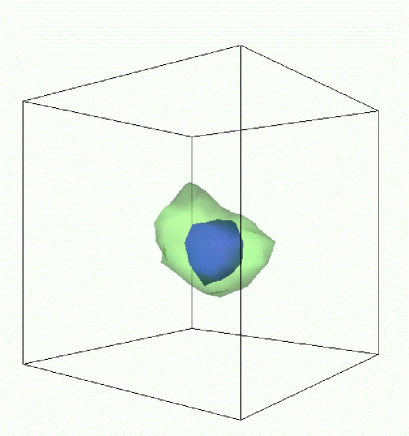
Figure 1: Isosurfaces ${\rm Tr}\,\Phi^{2}=3.89$ (green) and $\sum_{i<j}(1-{\rm Tr}U_{ij}/2)=0.18$ (blue) in a typical field configuration at $x=0.05$, $y=0.45$ and $\beta=18$. In order to reduce noise, the configuration was averaged over 50 subsequent Monte Carlo sweeps.

To illustrate that the twisted boundary conditions (17) indeed generate a monopole, we show in Fig. 1 the isosurfaces of ${\rm Tr}\,\Phi^{2}$ and the gauge action density $\sum_{i<j}(1-{\rm Tr}U_{ij}/2)$ in a typical field configuration at $x=0.05$, $y=0.45$ and $\beta=18$. The gauge action peaks and ${\rm Tr}\,\Phi^{2}$ dips around the same point, exactly as is expected to happen near the monopole core. Because of thermal fluctuations, the isosurfaces are not spherical.

IV.1 Observables

We measure the free energy and its derivative with respect to the scalar mass. The former is done via Eq. (22). In practice this does not work; the importance sampling of the theory with untwisted boundary conditions has very small overlap with that of the twisted partition function. This leads to strong sign fluctuations in $\Delta S$ which leads to a poor convergence of its average through Monte Carlo simulation.

Instead, as in Refs. Kajantie:1999zn ; Kovacs:2000sy ; Hoelbling:2001su , we can introduce a set of ensembles defined by a real parameter, $\varepsilon\in[0,1]$:

$$Z_{\varepsilon}\equiv\int DU_{i}D\Phi\exp\left(-S-\varepsilon\Delta S\right),$$ (34)

where $\varepsilon=0$ is the untwisted case, and $\varepsilon=1$ represents twisted boundary conditions. We then write

$$\Delta F=\int_{0}^{1}d\varepsilon\frac{\partial F_{\varepsilon}}{\partial\varepsilon}=\int_{0}^{1}d\varepsilon\langle\Delta S\rangle_{\varepsilon},$$ (35)

where the subscript $\varepsilon$ indicates that the expectation value must be measured using Eq. (34). This gives us the absolute value of $\Delta F$, but with the cost that we have to measure expectation values at non-physical values of $\varepsilon$. We call this the ‘method of progressive twisting’. Calculations of the free energy by progressive twisting typically used 10,000 to 20,000 measurements for each of 37 values of the twisting parameter, $\varepsilon$, which are then numerically integrated. (For an alternative approach, see Ref. deForcrand:2001fi .)

Alternatively, the derivative of the free energy, Eq. (23), may be measured directly, which avoids the reweighting problem. We are, however, calculating an intensive quantity as the difference of two approximately extensive numbers. Maintaining a constant error on the former demands increasing accuracy in the latter for increasing volume. Even allowing for self–averaging and the good scaling properties of the simulation algorithm, maintaining comparable precision in the free energy derivative requires CPU time rising as $L^{6}$. This limits the results of this study to $L\leq 46$. Calculations of the derivative with respect to the scalar mass used between 200,000 and 500,000 measurements for each of the boundary condition choices.

IV.2 Lattice parameters

$x$	$y$	$\beta$	$ag_{3}^{2}$	$L$
0.35	$-10$, $-3$, $-1$, $-0.5$, 1, 10	$18.0$	$0.222$	16

Table 1: Lattices used to study the monopole free energy by the method of progressive twisting.

$x$	$y$	$\beta$	$ag_{3}^{2}$	$L$
0.35	$-0.124$	4.5	0.889	4, 6, 8, 10, 12, 14, 16, 18, 20,
				22, 24, 28, 32, 36, 40, 46
		6.0	0.667	4, 6, 8, 10
		9.0	0.444	4, 6, 8, 10, 12, 14, 16
		12.0	0.333	4, 6, 8, 10, 12, 14, 16, 20
		18.0	0.222	4, 6, 8, 10, 12, 14, 16, 20

Table 2: Lattices used to study the system size dependence of the derivative of the monopole free energy.

The physical and lattice parameter values used are listed for reference in Tables 1 and 2.

In this section we discuss simulations of the SU(2) Georgi–Glashow model in three Euclidean dimensions. The action for the theory has been given in Eq. (5). In addition to the parameters that define our theory in the continuum limit, $x$ and $y$, there are two additional complications in the lattice theory, being the lattice spacing, $ag_{3}^{2}$, and the volume, $(ag_{3}^{2}L)^{3}$, of the cubic lattice on which we perform the simulations.

Detailed investigations of finite volume effects and scaling of correlation lengths have been performed for the $d=2+1$ pure gauge SU(2) and Georgi–Glashow field theories in teper98 ; hart99 . Here we summarise the findings briefly for the benefit of non–specialist readers.

The lattice calculations yield dimensionless results, which may be interpreted as being the physical result multiplied by the lattice spacing raised to their naïve dimensions, and which we denote via a circumflex accent. We remove the dependence on the unknown lattice spacing by multiplying the result with the appropriate power of $\beta=4/(ag_{3}^{2})$, and therefore it is natural to express the results in terms of powers of $g_{3}$, which has the dimensions of (mass)^1/2. For sufficiently fine lattices, the agreement with the continuum limit will be within the statistical errors of the lattice data, but on coarser lattices there may in principle be deviations. The results in Refs. teper98 ; hart99 are indicative of the continuum limit for $\beta\gtrsim 4.5$, which includes relatively coarse lattices at the lower end of this range (as we discuss later).

The lattice theory in Eq. (5) is parameterised by three couplings $(m^{2},\lambda,\beta)$. In order to vary the lattice spacing, we wish to change $\beta$ whilst maintaining the same continuum theory [i.e. $(x,y)$]. This is commonly referred to as moving along ‘lines of constant physics’. These trajectories have been calculated Laine:1995ag ; laine97 in the limit $\beta\rightarrow\infty$, and they are believed to be valid for lattices finer than $\beta\simeq 4.5-5.0$:

$$\beta = \frac{4}{ag_{3}^{2}},$$

$$\lambda = xg_{3}^{2},$$

$$\frac{m^{2}}{g_{3}^{4}} \approx y-\left(4+5x\right)\frac{3.1759}{4\pi ag_{3}^{2}}$$ (36)

$$-\frac{1}{16\pi^{2}}\Biggl{[}\left(20x-10x^{2}\right)\left(\ln\frac{6}{ag_{3}^{2}}+0.09\right)$$

$$~{}~{}~{}~{}~{}~{}~{}~{}~{}~{}+11.6x+8.7\Biggr{]}.$$

Again, we address the range of applicability in a later section. We are primarily interested in testing the idea that the ’t Hooft–Polyakov monopoles condense. The measurement of this is a fine balance. Whilst monopoles are topologically stable even if their core is smaller than the lattice spacing, it should be much larger than that to ensure they resemble the semiclassical ’t Hooft–Polyakov solution. Experience indicates that the correlation lengths of the gauge and scalar field should be at least 2 or 3 lattice spacings. Simultaneously, in order to see the screening of the free energy that signals the formation of the plasma, we require lattices that are (much) larger than the mean separation of the monopoles, such that it is possible for screening of magnetic charge to occur. Given that these two scales may be widely separated, it is not at all clear that we will be able to achieve the balance using a lattice size, $L$, which can be realistically simulated on the resources available.

We can use the known, semi-classical description of the monopoles Polyakov:1977fu to estimate the parameters needed for the lattice. Such estimates are, of course, only expected to be accurate up to numerical factors which may be important here. Nonetheless, we may hope the results are indicative at least, and the exercise gives some insight into the possible screening mechanism.

The monopole density (29) has a maximum value of just under $0.000345$. Screening will become apparent when the physical volume, $g_{3}^{6}V\equiv\left(4L/\beta\right)^{3}$, is such that $\nu_{0}V_{c}=1$; this yields

$$\frac{4L_{c}}{\beta} \gtrsim \left(\left.\frac{\nu_{0}}{g_{3}^{6}}\right|_{\rm max}\right)^{-\frac{1}{3}},$$ (37)

$$L_{c} \gtrsim 3.56\beta.$$ (38)

If a conservative value of $L_{c}=16$ is chosen to allow for possible suppression of the monopole density, this indicates that the gauge coupling is restricted to be $\beta\leq 4.5$. Our primary interest is in observing the monopole screening, so it is not strictly necessary that the perturbative lines of constant physics still hold on our lattices. We would like to maintain some contact with continuum physics, however, and thus go no lower than $\beta=4.5$.

Using Eq. (29), the maximum monopole density is reached for $v/g_{3}=0.421$. We are most interested in the fate of the monopole mass in the region of the phase diagram where there is a crossover between the two phases. For this reason we select $x=0.35$, and thus $y=-0.124$. At this parameter set, the gauge correlation length is, in units of the lattice spacing,

$$\hat{\xi}_{g}=\frac{\beta}{4}\left(\frac{v}{g_{3}}\right)^{-1}=2.67,$$ (39)

and the scalar field correlation length is

$$\hat{\xi}_{s}=\frac{\beta}{4}\left(\sqrt{-y}\right)^{-1}=3.20,$$ (40)

which are both suitably larger than the lattice grid size. Finer lattices were used to resolve better the small volume behaviour.

V Results

V.1 Small volumes

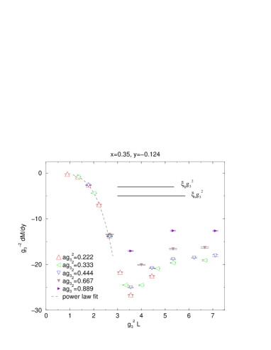
Figure 2: The derivative of the monopole free energy as a function of (small) lattice size at $x=0.35,y=-0.124$.

As discussed in Sect. III.1 the free energy $\Delta F$ is expected to be proportional to the volume of the system when $L\lesssim\xi$. We studied this in our simulations by measuring its $y$-derivative with couplings $x=0.35$ and $y=-0.124$. Obviously, this should behave in the same way as the free energy difference itself. The results from lattices of different sizes and different lattice spacings are plotted in Fig. 2 as functions of the physical lattice size $ag_{3}^{2}L$. At small $L$ the data show very little scaling violation. This suggests that we are not seeing a physically interesting effect here and supports the idea that the behaviour with $L$ has a simple origin. We show a fit of the form $-d_{0}L^{d_{1}}$, where $d_{\{0,1\}}$ are free parameters. Whilst the power law fits well by eye, the precise nature of the data makes the fits all quite poor ($\chi^{2}/{\rm dof}\gtrsim 5$). The fit shown is to the $\beta=18.0$ data only, and gives $d_{1}=4.2\,(5)$. Whilst not precisely 3, this gives qualitative support to our simple picture.

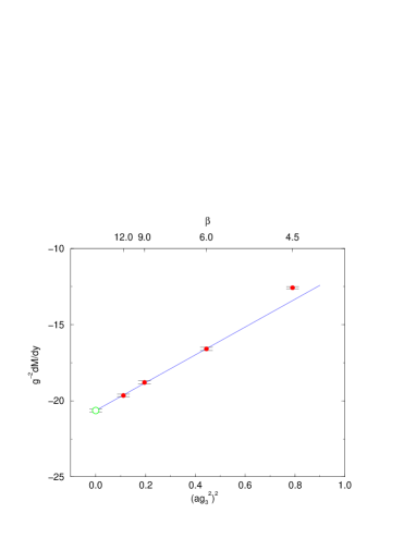
Figure 3: Continuum limit of the derivative of the free energy at $x=0.35$, $y=-0.124$ for fixed physical volume, $g_{3}^{2}L=5.3$.

Beyond $g_{3}^{2}L\simeq 3.5$ we see different behaviour. The derivative now decreases towards a plateau on intermediate scales. Whilst this decay may be a power law, we find the data insufficient to support a precise fit. The value of the plateau does show evidence of a discretisation effect. We may attempt to quantify this through a continuum extrapolation of the data at $g_{3}^{2}L=5.3$, admittedly still in the transient region, but where we have results for four couplings. We show the data in Fig. 3, along with a fit assuming only a leading order correction to scaling that is quadratic in the lattice spacing. This describes the data $\beta\geq 6.0$ well (with $\chi^{2}/{\rm dof}=0.178$). Even $\beta=4.5$ only deviates from this line by 7%, which backs up our previous statements on scaling and the applicability of the perturbative lines of constant physics (used to maintain constant $x,y$ as we varied $\beta$). In addition, this fit suggests that residual lattice spacing corrections are indeed very small at $\beta=18$, being around 2% in this case.

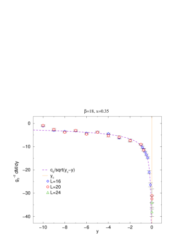
Figure 4: The derivative of the monopole free energy for intermediate system sizes for fixed $x$. Also shown is the a semiclassically inspired fit to the data.

In the region of intermediate volumes, when the twisted lattice supports a single monopole, we may attempt to measure the mass directly, to test the applicability of the semiclassical results to fully quantised excitations. We have two methods of approaching this. Less prone to statistical uncertainty is to use measurements of the derivative of the mass $dM/dy$ over a range in $y$ at fixed $x$. We make a ‘mean field’ assumption that we can describe this data using the formulæ of Section III, allowing for a shift in the phase transition by the substitution $y\to y-y_{c}$. Typical data, with such a fit, are shown in Fig. 4. The mean field assumption fits the data well, and from the coefficient $c_{0}$ we may extract a value for the radiatively corrected ’t Hooft function. We find $y_{c}$ to be consistent with zero for $x=0.35$.

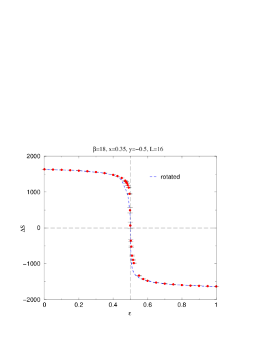
Figure 5: Measuring the monopole free energy by progressive twisting of an intermediately–sized system. We show a 180 degree rotation of the data to highlight the asymmetry.

Alternatively, we can measure the mass directly by the method of progressive twisting for fixed $x,y$. We show such a calculation in Fig. 5. The dominant error arises from the almost complete cancellation of the areas under the curve either side of $\varepsilon=0.5$. To illustrate this we plot also the same curve rotated through $180^{\circ}$.

$x$	method	$y$	$M/g_{3}^{2}$	$f(x)$	$\beta$	$L$
0.05	deriv.	—		1.066 (11)	18.0	$16-20$
0.35	deriv.	—		1.257 (14)	18.0	$16-24$
0.35	prog. twist	$-10$	50.8 (14.4)	1.07 (31)	18.0	$16$
0.35	prog. twist	$-3$	33.3 (5.5)	1.28 (22)	18.0	$16$
0.35	prog. twist	$-1$	18.2 (4.7)	1.21 (32)	18.0	$16$
0.35	prog. twist	$-0.5$	13.4 (1.9)	1.26 (18)	18.0	$16$
0.35	prog. twist	$1$	1.4 (2.1)	—	18.0	$16$
0.35	prog. twist	$10$	1.5 (1.2)	—	18.0	$16$
0.35	prog. twist	$-0.124$	2.8 (1.6)	0.53 (31)	4.5	$16$
0.35	prog. twist	$-0.124$	5.8 (1.8)	1.10 (35)	9.0	$16$
0.35	prog. twist	$-0.124$	6.3 (2.4)	1.19 (46)	12.0	$16$

Table 3: Estimates of the monopole mass and the ’t Hooft function.

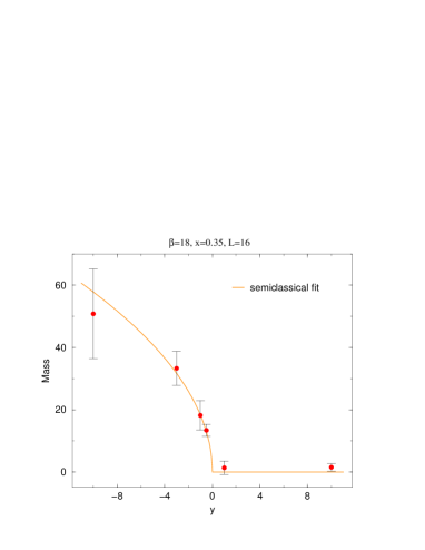
Figure 6: The monopole free energy as a function of $y$ for intermediately sized system. A semiclassically inspired fit is show, giving a value of the ’t Hooft function.

We summarise these estimates of $f(x)$ in Table 3, and in Fig. 6 where we show a fit to different $y$ as per Eq. (27). The masses and their derivatives behave much as the semiclassical expectations. Similarly the ’t Hooft function, within the limits of our statistical errors, does not appear to differ markedly due to radiative corrections. There is, however, a considerable variation in the data at $y=-0.124$ as we change $\beta$, and we may worry about systematic effects in our results. The first source of these is discretisation effects. The majority of our estimates are for $\beta=18.0$, and as we have argued above, the residual lattice spacing effects are small here. The variation in $\beta$ in the table is also in part due to a corresponding change in the physical volume of the system, and we may ask whether all our measurements are for ‘plateau’ masses uncontaminated by the transient small volume effects. We believe such biases to be small, especially for the $y\leq-1$. As we vary $y$ in Fig. 4 there is a great change in the correlation lengths $\xi_{\{s,g\}}$ for fixed volume. That the different effective volumes considered agree suggests we are indeed seeing the intermediate plateau unaffected by small $L$ transients. We are thus confident that our errors on these estimates of $f(x)$ are accurate. The joint fit in Fig. 6 yields $f(0.35)=1.23\,(12)$.

V.2 Intermediate and large volumes

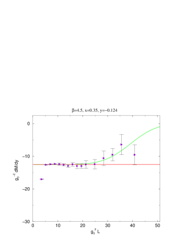
Figure 7: The derivative of the monopole free energy as a function of lattice size at $\beta=4.5,x=0.35,y=-0.124$. Also shown are fits assuming no screening and a dilute gas screening picture.

The large to intermediate system size data for the derivative of the free energy are shown in Fig. 7. For intermediate system size it is clear that the data is well represented by a constant independent of the lattice size, and we use such a hypothesis:

$$\frac{1}{g_{3}^{2}}\frac{\partial}{\partial y}\frac{M}{g_{3}^{2}}=c_{0}$$ (41)

where we expect the parameter $c_{0}$ to be $p_{0}/g_{3}^{2}$. We show such fits in Table 4. Our method is to begin with a low upper limit for the fitting range, and to then increase this, including progressively more data in the fit. The $\chi^{2}$ per degree of freedom and $Q$ (if our fitted form is the correct model, the probability that our data could have arisen as random fluctuations around that model) remain (very) acceptable up to $L\sim 40$. It is clear that beyond this the fits become unacceptable: the behaviour has changed as a consequence of screening.

$L_{\rm low}$	$L_{\rm high}$	$N_{\rm dof}$	$c_{0}$		$\chi^{2}/{\rm dof}$		$Q$
6	32	10	12.	431 (58)	0.	686	0.	722
6	36	11	12.	426 (58)	1.	106	0.	353
6	40	12	12.	421 (58)	1.	704	0.	066
6	46	13	12.	419 (58)	1.	813	0.	040
10	32	8	12.	705 (82)	0.	772	0.	628
10	36	9	12.	689 (82)	1.	229	0.	272
10	40	10	12.	677 (82)	1.	873	0.	044
10	46	11	12.	671 (82)	1.	976	0.	027

Table 4: Fitting the derivative of the free energy with an unscreened ansatz in Eq. (41).

We can attempt to describe the screening by fitting over a similar range using a fitting ansatz suggested by the dilute gas model:

$$\frac{1}{g_{3}^{2}}\frac{\partial}{\partial y}\frac{M}{g_{3}^{2}}=4c_{0}c_{1}(ag_{3}^{2}L)^{3}\frac{e^{-2c_{1}(ag_{3}^{2}L)^{3}}}{1-e^{-4c_{1}(ag_{3}^{2}L)^{3}}}$$ (42)

where $c_{0}$ is as before, and $c_{1}=\nu_{0}/g_{3}^{6}$. We show such fits over similar ranges in Table 5. For intermediate $L$ the fits are similar to those obtained using just a constant description. As data from larger systems is included, however, we see that the ansatz now remains good. A comparison of the two fits is plotted in Fig. 7.

$L_{\rm low}$	$L_{\rm high}$	$N_{\rm dof}$	$c_{0}$		$c_{1}(\times 10^{5}$)		$\chi^{2}/{\rm dof}$		$Q$
6	32	9	12.	499 (44)	0.	151 (93)	0.	938	0.	490
6	36	10	12.	500 (44)	0.	187 (40)	0.	867	0.	564
6	40	11	12.	502 (44)	0.	202 (35)	0.	826	0.	614
10	32	7	12.	445 (83)	1.	36 (106)	0.	816	0.	582
10	36	8	12.	451 (83)	1.	82 (47)	0.	753	0.	675
10	40	9	12.	454 (83)	1.	99 (37)	0.	722	0.	689
10	46	10	12.	449 (83)	1.	79 (35)	0.	773	0.	655

Table 5: Fitting the derivative of the free energy with a dilute gas screening ansatz in Eq. ((42).

We may calculate from $c_{1}$ the mean density of monopoles, $\nu_{0}/g_{3}^{6}=1.3\,(3)\times 10^{-5}$, which makes their mean separation

$$g_{3}^{2}D=42.6\,(3.3)$$ (43)

or, in lattice units at $\beta=4.5$, $\hat{D}=47.8\,(3.7)$. From this it is clear that we have not got the lattice volume necessary to see a complete screening of the free energy at $L\gg\hat{D}$. We cannot therefore completely rule out from our data the possibility that $\Delta F$ remains finite even in the infinite volume limit.

As was seen for small system sizes, the plateau values at least are heavily influenced by discretisation effects at $\beta=4.5$. To perform a scaling study of the screening mechanism is beyond our current means. Nonetheless, for a demonstration of the mechanism such effects are immaterial and do not affect the qualitative arguments.

Note also that no attempt has been made to estimate here the systematic errors in the monopole density. To do so would require a comparison of different screening hypotheses and fit functions, something that the data is, unfortunately, not accurate enough to address satisfactorily.

VI Conclusions

In this paper, we have used a fully non-perturbative technique to measure the free energy of a ’t Hooft–Polyakov monopole in the three–dimensional Georgi–Glashow model. This was achieved by simulating systems with two different boundary conditions, both of which are periodic up to symmetries of the Lagrangian. This preserves the lattice translation invariance of the system and therefore makes sure there are no boundary effects.

We found that in the Higgs phase, the free energy reached a constant value at intermediate volumes, which shows that it is associated with a localised object. This is the quantum analogue of the ’t Hooft–Polyakov monopole. We measure its mass by two different methods, and find it compatible with semiclassical expectations. ‘Mean field’ application of the classical relations appears successful, and we can make estimates of the quantum corrected ’t Hooft function. Our best estimates are $f(0.05)=1.066\,(11)$ and $f(0.35)=1.257\,(14)$ from the derivative of the mass with respect to $y$, and $f(0.35)=1.23\,(12)$ by the method of progressive twisting. These estimates are both self–consistent, and in agreement with the classical variation $f(x)\simeq 1+x$ for small $x$ goddard78 , indicating that radiative corrections are small.

When the volume increased above a certain critical value, however, the free energy started to approach zero. This is consistent with an analytical calculation within the dilute monopole gas approximation, which predicts that the free energy vanishes in the infinite volume limit at any values of the couplings.

In the dual superconductor picture, the vanishing monopole free energy implies confinement, and therefore our results are numerical evidence for Polyakov’s prediction that the Higgs phase of this theory is confining. Furthermore, if the monopole free energy vanishes everywhere, it cannot be used as an order parameter, and therefore our results strongly support the conjecture that the confining and Higgs phases are analytically connected to one another.

Neither, of course, can the monopole mass measured from the plateau in the free energy for intermediate system sizes act to distinguish the phases. It is non-zero in the deep Higgs phase and zero in the deep symmetric phase. This plateau does not exist, however, everywhere in the phase diagram, notably near the transition line itself. The mean monopole separation there will be comparable to the core size and no plateau would be observed. Thus the ‘mass’ is ill–defined and cannot serve as an order parameter.

Our findings suggest a straightforward generalisation to other cases. In a Euclidean formulation in any number of dimensions, any point-like topological defect that has finite action, will always have a non-zero density at any non-zero temperature. This means that these objects always have a zero free energy. An extended topological defect, such as a string or a domain wall, is, however, either a closed loop, surface etc., in which case it does not contribute to the global properties of the systems, or it has an infinite action. In the latter case, the fluctuations cannot generate them, and their free energy remains non-zero even in the infinite volume limit. Because the free energy can be used as an order parameter, this suggests that models with extended topological defects always have a true phase transition rather than a smooth crossover. This question will be studied further in a future publication.

- (1) G. ’t Hooft, Nucl. Phys. B 79 (1974) 276.
- (2) A. M. Polyakov, JETP Lett. 20 (1974) 194.
- (3) E. Fradkin and S. H. Shenker, Phys. Rev. D 19 (1979) 3682.
- (4) S. Nadkarni, Phys. Rev. Lett. 60 (1988) 491; Nucl. Phys. B 334 (1990) 559.
- (5) A. Hart, O. Philipsen, J. D. Stack and M. Teper, Phys. Lett. B 396 (1997) 217 eprint [hep-lat/9612021].
- (6) K. Kajantie, M. Laine, K. Rummukainen and M. Shaposhnikov, Nucl. Phys. B 503 (1997) 357 eprint [hep-ph/9704416].
- (7) H. Kleinert, Lett. Nuovo Cim. 35 (1982) 405.
- (8) A. Kovner, B. Rosenstein and D. Eliezer, Nucl. Phys. B 350 (1991) 325.
- (9) K. Kajantie, M. Laine, T. Neuhaus, J. Peisa, A. Rajantie and K. Rummukainen, Nucl. Phys. B 546 (1999) 351 eprint [hep-ph/9809334].
- (10) A. C. Davis, T. W. B. Kibble, A. Rajantie and H. Shanahan, JHEP 0011 (2000) 010 eprint [hep-lat/0009037].
- (11) A. M. Polyakov, Nucl. Phys. B 120 (1977) 429.
- (12) A. M. Polyakov, Gauge Fields and Strings (Harwood, 1987).
- (13) G. ’t Hooft, in “High Energy Physics”, EPS International Conference, Palermo 1975, ed. A. Zichichi; S. Mandelstam, Phys. Rept. 23 (1976) 245.
- (14) K. Kajantie, M. Laine, K. Rummukainen and M. Shaposhnikov, Nucl. Phys. B 458 (1996) 90 eprint [hep-ph/9508379].
- (15) A. Hart and O. Philipsen, Nucl. Phys. B 572 (2000) 243 eprint [hep-lat/9908041]; A. Hart, M. Laine and O. Philipsen. Nucl. Phys. B 586 (2000) 443 eprint [hep-ph/0004060]; Phys. Lett. B 505 (2001) 141 eprint [hep-lat/0010008].
- (16) G. ’t Hooft, Nucl. Phys. B 190 (1981) 455.
- (17) J. Smit and A. J. van der Sijs, Nucl. Phys. B 422 (1994) 349 eprint [hep-lat/9312087].
- (18) L. Del Debbio, A. Di Giacomo and G. Paffuti, Phys. Lett. B 349 (1995) 513 eprint [hep-lat/9403013]; A. Di Giacomo, B. Lucini, L. Montesi and G. Paffuti, Phys. Rev. D 61 (2000) 034503 eprint [hep-lat/9906024].
- (19) J. Fröhlich and P. A. Marchetti, Nucl. Phys. B 551 (1999) 770 eprint [hep-lat/9812004].
- (20) P. Cea and L. Cosmai, Phys. Rev. D 62 (2000) 094510 eprint [hep-lat/0006007].
- (21) K. Farakos, K. Kajantie, K. Rummukainen and M. Shaposhnikov, Nucl. Phys. B 442 (1995) 317 eprint [hep-lat/9412091].
- (22) M. Laine, Nucl. Phys. B 451 (1995) 484 eprint [hep-lat/9504001].
- (23) M. Laine and A. Rajantie, Nucl. Phys. B 513 (1998) 471 eprint [hep-lat/9705003].
- (24) A. S. Kronfeld and U. J. Wiese, Nucl. Phys. B 357 (1991) 521; Nucl. Phys. B 401 (1993) 190 eprint [hep-lat/9210008].
- (25) G. ’t Hooft, Nucl. Phys. B 138 (1978) 1.
- (26) T. G. Kovacs and E. T. Tomboulis, Phys. Rev. Lett. 85 (2000) 704 eprint [hep-lat/0002004].
- (27) C. Hoelbling, C. Rebbi and V. A. Rubakov, Phys. Rev. D 63 (2001) 034506 eprint [hep-lat/0003010].
- (28) A. Hart, B. Lucini, Z. Schram and M. Teper, JHEP 11 (2000) 043 eprint [hep-lat/0010010].
- (29) P. de Forcrand, M. D’Elia and M. Pepe, Phys. Rev. Lett. 86 (2001) 1438 eprint [hep-lat/0007034].
- (30) M. N. Chernodub, F. V. Gubarev, M. I. Polikarpov and V. I. Zakharov, Phys. Lett. B 514 (2001) 88 eprint [hep-ph/0101012].
- (31) P. Goddard and D. I. Olive, Rept. Prog. Phys. 41 (1978) 1357.
- (32) A. Hart, B. Lucini, Z. Schram and M. Teper, JHEP 06 (2000) 040 eprint [hep-lat/0005010].
- (33) M. Teper, Phys. Rev. D 59 (1999) 014512 eprint [hep-lat/9804008].