Hadronic Correlators from All-point Quark Propagators

Abstract

A method for computing all-point quark propagators is applied to a variety of processes of physical interest in lattice QCD. The method allows, for example, efficient calculation of disconnected parts and full momentum-space 2 and 3 point functions. Examples discussed include: extraction of chiral Lagrangian parameters from current correlators, the pion form factor, and the unquenched eta-prime.

1 Methodology

The very high cost of generating decorrelated dynamical gauge configurations makes it increasingly important to extract the maximum physical information content of each available configuration. In many cases, this requires calculation of hadronic observables involving quark propagators from any point on the lattice to any other. Here we describe an approach to obtaining such propagators by simulating bosonic pseudofermion fields. Introduce bosonic pseudofermion field $\phi_{ma}$ with action ($m$ a lattice site, $a$ the spin-color index, $Q$ the Wilson or clover operator):

$$S(\phi) = \phi^{\dagger}Q^{\dagger}Q\phi$$

$$= \phi^{\dagger}H^{2}\phi,\;\;\;H\equiv\gamma_{5}Q=H^{\dagger}$$

For fixed background gauge field $A$, simulating the pseudofermion field with the preceding action produces the following correlator ($<<O>>$ means the average of $O$ relative to the measure $e^{-S}$) :

$$<<\phi_{ma}\phi^{*}_{nb}>>_{S(\phi)} = (H^{-2})_{ma,nb}$$

$$<<\phi_{ma}(\phi^{\dagger}H)_{nb}>>_{S(\phi)} = (H^{-1})_{ma,nb}$$

$$= (Q^{-1}\gamma_{5})_{ma,nb}$$

These simulations are practical for two reasons:
(i) The pseudofermion average $<<....>>$ is efficiently implemented by heat-bath update of pseudofermion fields.
(ii) For a fixed gauge field, most quantities decorrelate after a few pseudofermion sweeps.
The computation of multipoint hadronic correlators involving $n$ quark propagators can be reduced to convolutions of $n$ pseudofermion fields, rapidly computed by fast Fourier transform (FFT). For example, the full 4-momentum transform $\Delta(q)\equiv\sum_{x,y}e^{iq\cdot(x-y)}\Delta(x,y)$ of the 2-point pseudoscalar correlator

$$\Delta(x,y) = <0|T\{\bar{\Psi}(x)\gamma_{5}\Psi(x)\;\bar{\Psi}(y)\gamma_{5}\Psi(y)\}|0>$$

$$= -<\rm{tr}((Q^{-1}\gamma_{5})_{xy}(Q^{-1}\gamma_{5})_{yx})>$$

$$= -<<\sum_{ab}\phi_{xa}(\phi^{\dagger}H)_{yb}\chi_{yb}(\chi^{\dagger}H)_{xa}>>$$

$$= -<<(\phi^{\dagger}H\chi)_{yy}(\chi^{\dagger}H\phi)_{xx}>>$$

becomes

$$\Delta(q)=-<<\rm{FFT}(\chi^{\dagger}H\phi)(q)\rm{FFT}(\phi^{\dagger}H\chi)(-q)>>$$

2 Applications

We have studied the feasibility of a pseudofermion approach to all-point propagators in a number of examples of physical interest. A brief report on the progress to date follows.

2.1 Chiral Lagrangian Parameters from Current Correlators

The chiral Lagrangian predicts the low-momentum structure of 2-point functions such as $\Delta(q)$ in QCD [1]:

$$\Delta(q) \simeq \frac{G_{\pi}^{2}}{q^{2}+M_{\pi}^{2}}+\frac{B^{2}}{2\pi^{2}}(h_{1}-l_{4})+Cq^{2}+O(q^{4})$$

$$G_{\pi} = \frac{F_{\pi}M_{\pi}^{2}}{m_{q}}$$

$$BF_{\pi}^{2} = <\bar{\Psi}\Psi>$$

We have studied various correlators of this type using 800 dynamical configurations generated using the truncated determinant (TDA) algorithm [2] on large coarse (6⁴) lattices. The presence of low eigenmodes of $H$ leads to longer autocorrelation times for the zero momentum component (see Fig.1), on the order of 60 pseudofermion sweeps, with much more rapid decorrelation for nonzero momentum values of $\Delta(q^{2})$. (Low momentum autocorrelations can be substantially reduced by projecting out the lowest few eigenmodes of $H$- the required code has been written and is presently being tested [3]). However, even at zero momentum, the intrinsic gauge fluctuations exceed the statistical errors from the pseudofermion evaluation (which become very small at higher momenta where decorrelation is rapid). This can be seen in Fig.2, where we display the measured $\Delta(q^{2})$ for two separate configurations, as well as the average over 800 configurations and a fit to the chiral formula. In fact a good fit to the predicted chiral form can be obtained even without the zero-momentum point.

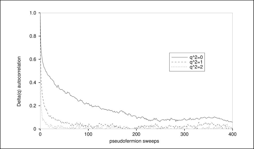
Figure 1: Decorrelation of pseudofermion evaluations of $\Delta(q)$

The parameters $h_{1},l_{4}$ are couplings in the next-to-leading order chiral Lagrangian [1]. Fitting the measured $\Delta(q)$ (800 6⁴ unquenched TDA lattices [4] with O($a^{2}$) improved gauge action, $a$=0.4 F):

$$\Delta(q)=\frac{A_{1}}{q^{2}+A_{2}}+A_{3}+A_{4}q^{2}+A_{5}(q^{2})^{2}$$

A standard cosh fit of smeared-local correlators gives $M_{\pi}=0.396\pm 0.007$. Allowing the pion mass to vary in the chiral formula, the best fit (see Fig.2) is obtained in the range 0.25$<q^{2}<$2.5 GeV², and gives a 2% evaluation (jackknife errors) of the one-loop chiral parameter $A_{3}$:

$$A_{1} = 23.1\pm 0.4$$

$$A_{2} = 0.178\pm 0.017\Rightarrow M_{\pi}=0.422\pm 0.020$$

$$A_{3} = 9.48\pm 0.16$$

$$A_{4} = -0.70\pm 0.02,\;\;A_{5}=0.025\pm 0.001$$

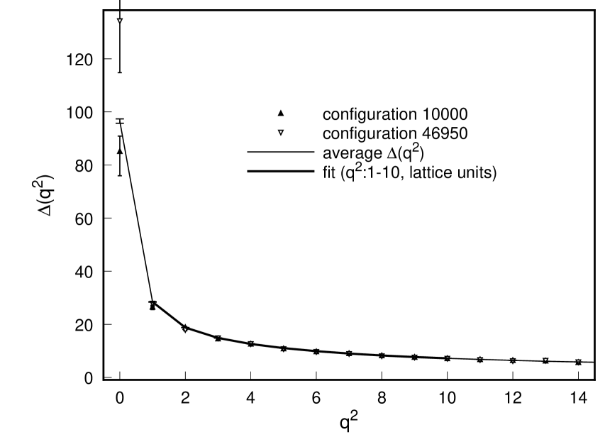
Figure 2: 4 parameter fit of measured $\Delta(q^{2})$

2.2 Three-point Functions: the Pion Form Factor

To extract the pion formfactor, we need the following 3-point function (see Fig.3):

$$J_{t_{0}t_{1}t_{2}}(\vec{q}^{2}) = \sum_{\vec{w}\vec{x}\vec{y}\vec{z}}e^{i\vec{q}\cdot(\vec{x}-\vec{y})}f^{\rm sm}(\vec{z})f^{\rm sm}(\vec{w})$$

$$<\bar{\Psi}(\vec{z}+\vec{x},t_{2})\gamma_{5}\Psi(\vec{x},t_{2})\bar{\Psi}(\vec{y},t_{1})\gamma_{0}\Psi(\vec{y},t_{1})$$

$$\bar{\Psi}(\vec{w},t_{0})\gamma_{5}\Psi(0,t_{0})>$$

Figure 3: 3-point function for pion form factor

To evaluate $J(q^{2})$ simultaneously for all spacelike $q$ injected at time $t_{1}$ by the electromagnetic current, it suffices to use a conventional smeared source propagator for the quark propagation from $\vec{w},t_{0}$ to $\vec{y},t_{1}$ and a smeared sink propagator for the propagation from $\vec{x}+\vec{z},t_{2}$ to $\vec{0},t_{0}$. The remaining propagator from $\vec{y},t_{1}$ to $\vec{x},t_{2}$ is then needed for all source and sink points (to obtain the full momentum space Fourier transform) and is evaluated by the pseudofermion technique. At this stage, both the connected and disconnected contributions (where the quark propagates from $\vec{y}$ back to $\vec{y}$) to $J(q^{2})$ are readily available, as the all-point propagator also gives us the amplitude for all coincident source and sink points. An approximate pion form factor is given by $J(q^{2})e^{(t_{2}-t_{1})E(q)}/E(q))$ ($t_{0},t_{1},t_{2}$=0,3,6, with $E(q)$ the energy for a lattice pion of momentum $q$): results obtained with 60 quenched 12³x24 lattices at $\beta=$5.9 are shown in Fig. 4. Analysis of a single gauge configuration takes about 12 hours on a Pentium 4 processor. Reliable calculation of the pion form factor requires use of optimized smearing wavefunctions $f^{\rm sm}$ to project out ground-state pions as the signal dies quickly at larger Euclidean times $t_{1}-t_{0},t_{2}-t_{1}$, especially at larger momentum, and to check that a plateau is reached at large Euclidean time. Of course, more accurate results require higher statistics than used in this feasibility study.

Figure 4: Connected and Disconnected contributions to Pion Form Factor

2.3 The unquenched eta-prime

We may extract the etaprime propagator in the isoscalar channel using two pseudofermion fields to generate propagators for both quark lines:

$$\Delta_{\eta}(p) = \sum_{xy\vec{z}\vec{w}}e^{ip\cdot(x-y)}f^{\rm sm}(\vec{z})f^{\rm sm}(\vec{w})\times$$

$$<\bar{\Psi}(\vec{z}+\vec{x},x_{4})\gamma_{5}\Psi(x)\bar{\Psi}(\vec{w}+\vec{y},y_{4})\gamma_{5}\Psi(y)>$$

In terms of pseudofermion averages, this gives a connected

$$\sum_{xy\vec{z}\vec{w}}e^{ip\cdot(x-y)}f^{\rm sm}(\vec{z})f^{\rm sm}(\vec{w})$$

$$<<\phi(x)(\phi^{\dagger}H)(y+\vec{w})\chi(y)(\chi^{\dagger}H)(x+\vec{z})>>$$

as well as disconnected (“hairpin”) contribution (for two flavors of sea quarks):

$$-2\sum_{xy\vec{z}\vec{w}}e^{ip\cdot(x-y)}f^{\rm sm}(\vec{z})f^{\rm sm}(\vec{w})$$

$$<<\phi(x)(\phi^{\dagger}H)(x+\vec{z})\chi(y)(\chi^{\dagger}H)(y+\vec{w})>>$$

Computations of the unquenched eta-prime propagator using this method are in progress, using 10³x20 lattices generated with the TDA algorithm.

References

• [1] J. Gasser, H. Leutwyler, Ann. Phys. 158,142(1984).
• [2] A. Duncan, E. Eichten, and H. Thacker, Phys. Rev. D59, 014505 (1998).
• [3] A. Duncan and E. Eichten, “Pseudofermion Approach to All-point Propagators”, in preparation.
• [4] Talk of E. Eichten, this conference.