QCD spectroscopy with three light quarks
Abstract
We report about a simulation using three dynamical Wilson quarks and on the progress in going to small quark masses.
1 INTRODUCTION
One of the main purposes of lattice QCD simulations is to predict the spectrum of QCD, i.e. masses and decay constants of the light hadrons. Due to computational and algorithmic limitations certain simplifications have to be made. The quenched approximation allows to reproduce the physical spectrum already up to systematic errors of 10%, as it was shown in detail in [1].
Lots of effort has been spent to increase the available computing power, see e.g. [2] for such a project, and to overcome algorithmic limitations [3]. There have been several large scale simulations of QCD with two dynamical, degenerate quarks [4], all based on the Hybrid Monte Carlo algorithm [5]. Still these simulations worked with relatively large quark masses. For phenomenological reasons it is crucial to go beyond this scenario and simulate with three dynamical quarks with masses eventually approaching the physical ones [6].
Some restrictions can be overcome by using variants of the multibosonic algorithm [7] like the two-step multibosonic (TSMB) algorithm [3]. The latter has already been used successfully in simulations of supersymmetric field theories [8] and finite density QCD [9].
In this contribution we present preliminary results from a first simulation using three dynamical Wilson quarks. The aim of these simulations is to achieve small quark masses and to estimate their influence on the spectrum.
2 SMALL MASSES
There are several problems when tuning the algorithms to small quark masses. One problem is the critical slowing down, which reflects the decreasing efficency at smaller masses. In [10] it has been shown that this problem is less severe with multibosonic algorithms than with the HMC algorithm. But still this can become a problem at too small masses. A first orientation can be obtained by making a comparison with previous simulations. In [11] TSMB has been used for the supersymmetric Yang-Mills theory where the number of flavour is . In that simulation condition numbers of occurred. Because the performance of the algorithm depends mainly on the condition number of the squared fermion matrix, and not on , one can similarly expect to reach condition numbers of at least for the case . This would correspond to quark masses of roughly . The polynomial orders and that are needed for the TSMB algorithm mainly depend on . Changing from to , is increasing by less than and by about . This dependence is reflected by the asymptotic estimate of for large [12]
| (1) |
where changes only slightly with and is the bare quark mass.
Another potential problem when approaching the chiral limit may be posed by a sign change of the fermionic determinant. This so-called sign problem may spoil the statistical signal of observables. Experience shows that both situations (with and without sign problem) are possible [13, 11]. The sign of the determinant can be controlled by the spectral flow of small eigenvalues. From this experience it is already clear that a sign change can only occur if there are extremly small eigenvalues (). Such eigenvalues did not appear in our runs so far, which gives a first evidence for the absence of the sign problem.
3 PARAMETER SPACE
The spectrum of the light hadrons can be studied in the confined phase, the phase below the finite temperature phase transition
| (2) |

On small lattices the transition between the two phases can be seen clearly, as e.g. in figure 1. The parameters of our simulations lead to
| (3) |
where is the Sommer scale parameter. Therefore we are safe from finite size effects due to deconfinement by choosing lattice sizes such that
| (4) |
The parameters we finally want to achieve are shown in table 1. These parameters give a constant volume and are such that , corresponding to a quark mass of . Since the volume and the quark mass are constant one can perform a continuum extrapolation from these points. In addition pion induced finite volume effects are under control as well, as they can be estimated by .
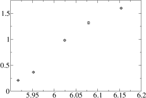
Results for our reference scale, the Sommer parameter , are presented in figure 2.

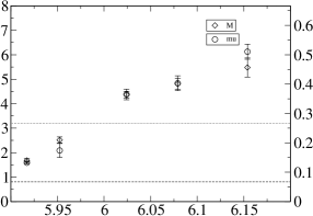
For tuning the parameters to the values in table 1 we further have to look at the pseudoscalar mass and the quark mass. This latter can be characterized by the dimensionless quantities
| (5) |
and
| (6) |
The two definitions become proportional to each other for small masses. First results are shown in figures 3 and 4. In figure 4 there are two horizontal lines indicating and the mass region we want to reach, . Depending on the size of the mass , and lattices have been used.
4 CONCLUSIONS AND OUTLOOK
We presented preliminary results from simulations with three dynamical quarks. The results show that it should be possible to reach small quark masses within the proposed settings. For the moment we are exploring the region below the strange quark mass.
ACKNOWLEDGMENTS
W.S. is supported by the DFG Graduiertenkolleg “Feldtheoretische Methoden in der Elementarteilchentheorie und Statistischen Physik”. The numerical productions were run on the APEmille systems installed at NIC Zeuthen, the Cray T3E systems at NIC Jülich, the ALiCE-cluster at Wuppertal University and the PC clusters at DESY Hamburg.
References
- [1] S. Aoki et al. [CP-PACS Collaboration], Phys. Rev. Lett. 84 (2000) 238-241.
- [2] H. Simma et al. [APE Collaboration], these proceedings.
- [3] I. Montvay, Nucl. Phys. B466 (1996) 259-284.
- [4] Th. Lippert, these proceedings; A. Ukawa, ibid; H. Wittig, ibid.
- [5] S. Duane, A. D. Kennedy, B. J. Pendleton, D. Roweth, Phys. Lett. B195 (1987) 216-222.
- [6] S. Sharpe, N. Shoresh, Phys. Rev. D62 (2000) 094503.
- [7] M. Lüscher, Nucl. Phys. B418 (1994) 637-648.
- [8] I. Campos et al. [DESY-Münster Collaboration], Eur. Phys. J. C11 (1999) 507-527.
- [9] S. Hands et al., Eur. Phys. J. C17 (2000) 285-302.
- [10] W. Schroers et al., hep-lat/0110033.
- [11] F. Farchioni et al., these proceedings.
- [12] I. Montvay, Comput. Phys. Commun. 109 (1998) 144-160.
- [13] L. Scorzato et al., these proceedings.