Measuring infrared contributions to the QCD pressure

Abstract

For the pressure (or free energy) of QCD, four-dimensional (4d) lattice data is available at zero baryon density up to a few times the critical temperature $T_{c}$. Perturbation theory, on the other hand, has serious convergence problems even at very high temperatures. In a combined analytical and three-dimensional (3d) lattice method, we show that it is possible to compute the QCD pressure from about $2T_{c}$ to infinity. The numerical accuracy is good enough to resolve in principle, e.g., logarithmic contributions related to 4-loop perturbation theory.

Introduction. The properties of QCD matter are expected to change above a critical temperature $T_{c}\sim$ 200 MeV. While the low-temperature phase is governed by bound states, such as mesons, the high-temperature phase should, due to asymptotic freedom, look more like a gas of free quarks and gluons. Any observable witnessing this change is therefore a potential candidate for direct or indirect measurements in heavy-ion collision experiments. One such observable is the free energy density, or pressure of the system, since according to the Stefan-Boltzmann law (i.e. neglecting interactions), it is proportional to the number of effective degrees of freedom.

For vanishing baryon density, at a temperature $T$ and volume $V$, the free energy density $f$ is simply given by the functional integral

$$f=-{\frac{T}{V}\,}\ln\!\int{\cal D}[A\bar{\psi}\psi]e^{-\!\int_{0}^{1/T}\!\!\!\!\!d\tau\int_{V}\!\!d^{3}x\,{\cal L}_{E}[A\bar{\psi}\psi]}\;,$$ (1)

where ${\cal L}_{E}$ is the standard QCD Lagrangian. For $V\to\infty$, the pressure $p$ is given by $p=-f$.

The most direct way to evaluate Eq. (1) is to measure it numerically on the lattice. This has been done by a number of groups, for zero as well as non-zero number of fermion flavours $N_{f}$ (e.g. [1, 2]). The general picture emerging is the following: The pressure rises sharply in the interval $(1-2)T_{c}$, to level off at a few times $T_{c}$. At the highest temperatures used in the simulations, typically $(4-5)T_{c}$, the deviation from the Stefan-Boltzmann limit is about $15\%$. At even higher temperatures, the pressure is then expected to asymptotically approach the ideal-gas value $p_{0}(T)=(\pi^{2}T^{4}/45)(N_{c}^{2}\!-\!1+(7/4)N_{c}N_{f})$, where $N_{c}$ denotes the number of colours.

The $15\%$ deviation cannot be systematically understood in terms of (finite-temperature) perturbation theory. While the expansion is known analytically to 5th order in the gauge coupling $g$ [3], convergence properties are extremely poor. Therefore, in the past few years a lot of effort has gone into refined and/or alternative analytic approaches [4]. A general feature of these works is the suppression of infrared effects. While this suppression does not seem to be crucial in the computation of the pressure, one might not be satisfied with accepting it as an ad hoc assumption. The aim of this talk is to briefly review our framework of resumming the infrared contributions to the pressure to all orders [5].

Pressure via effective theory. A way to understand the poor convergence of the ordinary perturbative expansion is the observation that when $gT\ll\pi T$, the system undergoes dimensional reduction (see, e.g., [6] and references therein). In the case of QCD, the effective theory is a 3d SU($N_{c}$) + adjoint Higgs model:

$${\cal L}_{\rm 3d}={\frac{1}{4}\,}F_{ij}^{2}+\!{\frac{1}{2}\,}\![D_{i},A_{0}]^{2}+\!{\frac{1}{2}\,}\!m^{2}_{3}A_{0}^{2}+\!{\frac{1}{4}\,}\!\lambda_{3}A_{0}^{4}.$$ (2)

The parameters ($g_{3}$, $m^{2}_{3}$, $\lambda_{3}$) are related to the physical parameters of the full 4d theory ($T$, ${\Lambda_{\overline{\rm MS}}}$) by perturbatively integrating out the hard modes ($\sim\pi T$). Below, we will work with the dimensionless variables $x=({\lambda_{3}}/{g_{3}^{2}})$ and $y=({m^{2}_{3}}/{g_{3}^{4}})$, known at next-to-leading order [7].

The effective theory is confining, hence non-perturbative [8]. Therefore, the only way to systematically include the infrared contributions to the pressure is to treat ${\cal L}_{\rm 3d}$ on the lattice.

Let us rewrite the pressure, up to hard-scale $g^{6}$ contributions, as

$${\frac{p(T)}{p_{0}(T)}\,}=1-{\frac{5x}{2}\,}-{\frac{45}{8\pi^{2}}\,}\left({\frac{g_{3}^{2}}{T}\,}\right)^{3}\left[{\cal F}_{\overline{\rm MS}}(x,y)\vphantom{{\frac{1}{1}\,}}\right.$$

$$\left.{}-{\frac{24y}{(4\pi)^{2}}\,}\left(\ln{\frac{\bar{\mu}_{\rm{3d}}}{T}\,}+\delta\right)\right]\;,$$ (3)

where $\delta\sim 10^{-4}$, $p_{0}(T)$ is the Stefan-Boltzmann value, and the dependence on the scale $\bar{\mu}_{\rm{3d}}$, which originates from an infrared divergence of the 4d part, cancels against an ultraviolet term in the dimensionless 3d free energy density ${\cal F}_{\overline{\rm MS}}(x,y)$. We write ${\cal F}_{\overline{\rm MS}}(x,y)$ as

$${\cal F}_{\overline{\rm MS}}(x_{0},y_{0})+\!\int_{y_{0}}^{y}\!\!dy\left({\frac{\partial{\cal F}_{\overline{\rm MS}}}{\partial y}\,}\!+{\frac{dx}{dy}\,}{\frac{\partial{\cal F}_{\overline{\rm MS}}}{\partial x}\,}\right)\;,$$ (4)

and aim at measuring it on the lattice. This requires a determination of the quadratic and quartic Higgs field condensates (which equal the partial derivatives under the integral), as well as a (4-loop) perturbative computation in lattice regularization, to match to the ${\overline{\mbox{\rm MS}}}$ scheme. We choose to fix the integration constant ${\cal F}_{\overline{\rm MS}}(x_{0},y_{0})$ at high temperatures $T\sim 10^{11}T_{c}$, where one is confident that continuum perturbation theory converges.

As a first result obtained along the strategy outlined, Fig. 1 shows the normalized pressure. The integration constant has been fixed perturbatively on the 3-loop level, allowing for an additional constant $e_{0}$, which represents an (up to now) unknown $g_{3}^{6}$ contribution. In principle, this constant can be determined in a setup equivalent to the above, after splitting off its perturbative part: A further reduction relates $e_{0}$ to the free energy of 3d pure gauge theory (see, e.g., [6]), which can be determined on the lattice. On the lattice side, we have only included the quadratic scalar condensate in Fig. 1, due to reasons explained in the next section; however, at $T\to T_{c}$ the quartic one will become important as well.

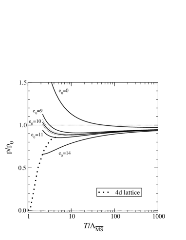
Figure 1: The pressure after the inclusion of the infrared part according to Eq. (4) (from Ref. [5]). Statistical errors are shown only for $e_{0}=10$.

3d lattice measurements. Let us now discuss in more detail how the actual measurement of the 3d condensates is carried out. We need to relate lattice and ${\overline{\mbox{\rm MS}}}$ regularization schemes. Here, the super-renormalizability of the 3d theory plays an important role: there are only a finite number of divergent terms, such that analytic relations can be computed exactly near the continuum limit [9]. Writing ${\beta_{\rm G}}=({2N_{c}}/{g_{3}^{2}a})$ where $a$ is the lattice spacing, the observables we need behave schematically like

$$\partial_{y}{\cal F}_{{\mbox{\scriptsize${\overline{\mbox{\rm MS}}}$}}}\sim\!\lim_{{\beta_{\rm G}}\to\infty}\!\left\{\left\langle{\rm Tr}A_{0}^{2}\right\rangle_{\rm L}\!+\!{\beta_{\rm G}}+\!\ln{\beta_{\rm G}}+\!1\right\},$$ (5)

$$\partial_{x}{\cal F}_{{\mbox{\scriptsize${\overline{\mbox{\rm MS}}}$}}}\sim\lim_{{\beta_{\rm G}}\to\infty}\left\{\left\langle({\rm Tr}A_{0}^{2})^{2}\right\rangle_{\rm L}+{\beta_{\rm G}}^{2}\mbox{\hskip 36.0pt}\right.$$

$$\left.\vphantom{1_{1}^{1}}{}+{\beta_{\rm G}}\ln{\beta_{\rm G}}+{\beta_{\rm G}}+\ln{\beta_{\rm G}}+1\right\}.$$ (6)

For Eq. (5) all three coefficients are known [10]. In the case of the quartic condensate, Eq. (6), all we know so far are the four divergent terms: the weakest logarithmic divergence can be obtained in a 4-loop continuum calculation, but the 4-loop lattice constant is still unknown. This is precisely the reason why in Fig. 1 only the effect of $\left\langle{\rm Tr}A_{0}^{2}\right\rangle_{\rm L}$ is included. While the graphs needed can be systematically generated [11], carrying out the lattice integrals remains a major challenge.

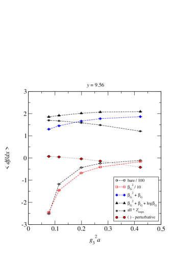
Figure 2: A measurement of one of the partial derivatives needed in Eq. (4), $\partial_{x}{\cal F}$, at a fixed $y$, as a function of the lattice spacing $g_{3}^{2}a$. Note that the raw data (open circles) is scaled by a factor 1/100. The other curves result from subtracting various divergences, Eq. (6); taking into account improvement [12]; and finally (filled circles), subtracting the perturbative value.

Nevertheless, we can show how the data involving the quartic condensate behaves. In Fig. 2, we demonstrate for one specific temperature that the series in Eq. (6) indeed regulates the lattice operator as $g_{3}^{2}a\to 0$. Indeed, taking into account successive terms of the series, one observes how the divergence at small $a$ becomes weaker. Note that while the continuum limit can be taken already now, the actual value of $\partial_{x}{\cal F}_{{\mbox{\scriptsize${\overline{\mbox{\rm MS}}}$}}}$ will have to await the above-mentioned 4-loop computation of the finite term in lattice regularization.

Conclusions. We wish to point out two trends seen in Fig. 1: First, the outcome is sensitive to the non-perturbative parameter $e_{0}$, which in principle can be determined by additional computations. Clearly, there exists a range for that parameter which leads to a sensible result.

Second, comparing with Fig. 1 of [5], at $T>30{\Lambda_{\overline{\rm MS}}}$ the curves for $g^{5}$ (denoted by $y^{{\frac{1}{2}\,}}$ there) and $e_{0}=10$ fall almost on top of each other, signalling a cancellation of all higher-order terms (determined by the quadratic Higgs condensate) against the large non-perturbative $g^{6}$ contribution. Hence, in this temperature range the pressure is indeed dominated by ultraviolet effects.

Let us also remark that as demonstrated in Fig. 2, 3d lattice results involve always a systematic extrapolation to the continuum limit, and are precise enough to resolve, e.g., logarithmic effects related to 4-loop perturbation theory.

We end by noting that the inclusion of $N_{f}$ fermion flavours as well as a baryon chemical potential $\mu_{b}$ pose no further complications, and hence provide for a natural extension of this investigation.

References

- [1] G. Boyd et al, Nucl. Phys. B 469 (’96) 419.
- [2] F. Karsch et al, Phys. Lett. B 478 (’00) 447.
- [3] C. Zhai and B. Kastening, Phys. Rev. D 52 (’95) 7232.
- [4] For a recent review, see J.-P. Blaizot and E. Iancu, hep-ph/0101103.
- [5] K. Kajantie et al, Phys. Rev. Lett. 86 (’01) 10.
- [6] E. Braaten and A. Nieto, Phys. Rev. D 53 (’96) 3421.
- [7] K. Kajantie et al, Nucl. Phys. B 503 (’97) 357.
- [8] D.J. Gross et al, Rev. Mod. Phys. 53 (’81) 43.
- [9] K. Farakos et al, Nucl. Phys. B 442 (’95) 317.
- [10] M. Laine and A. Rajantie, Nucl. Phys. B 513 (’98) 471.
- [11] K. Kajantie et al, hep-ph/0109100, and references therein.
- [12] G.D. Moore, Nucl. Phys. B 523 (’98) 569.