Novel Quantum Monte Carlo Algorithms for Fermions

Abstract

Recent research shows that the partition function for a class of models involving fermions can be written as a statistical mechanics of clusters with positive definite weights. This new representation of the model allows one to construct novel algorithms. We illustrate this through models consisting of fermions with and without spin. A Hubbard type model with both attractive and repulsive interactions becomes tractable using the new approach. Precision results in the two dimensional attractive model confirm a superfluid phase transition in the Kosterlitz-Thouless universality class.

1 Introduction

Fermion algorithms are known to be notoriously difficult. The main reason for this is that it is difficult to write the partition function of models involving fermions as a sum over configurations with positive definite weight. The most common approach is to integrate out the fermions in favor of a fermion determinant which leads to an effective bosonic partition function. Typically one obtains

$$Z\;=\;\int\;[d\phi]\;\exp\left(-S[\phi]\right)\;\mathrm{Det(M[\phi])}$$ (1)

where the determinant is a non-local function of the bosonic fields $[\phi]$. In cases where $\mathrm{Det(M[\phi])}$ is positive useful algorithms can be found [1-3]. In other cases one can make progress only by using uncontrolled approximations [4]. Thus it is important to find alternative approaches to fermionic path integrals.

Recently a novel approach to solve certain lattice fermionic models was discovered [5-11]. It is possible to rewrite the partition function of these models as a sum over configurations of local bond variables with positive definite weights. The bonds $b$ connect lattice sites and thus divide the lattice into clusters. The partition function can be written as

$$Z\;=\;\sum_{[b]}W[b]\;\overline{\mathrm{Sign}}[b]$$ (2)

where $W[b]>0$ is the magnitude of the Boltzmann weight for a given bond configuration, and $\overline{\mathrm{Sign}}[b]\geq 0$ is an entropy factor arising from “cluster flips” that result due to degrees of freedom other than the bonds”. This representation of the fermionic partition function allows one to construct efficient cluster algorithms which had previously been found only for bosonic problems. In this article we describe this new approach to fermionic path integrals and present a result from recent Monte-Carlo studies using the new method.

2 Fermion World-Line Path Integrals

Consider spin-less fermions, hopping on a $d$-dimensional cubic lattice consisting of $V=L^{d}$ sites and satisfying periodic or anti-periodic spatial boundary conditions. Let us focus on models whose Hamilton operators can be described by

$$H=\sum_{x,\hat{i}}h_{x,x+\hat{i}}$$ (3)

where $\hat{i}=1,2,..d$ represents directions and $h_{x,i}$ is a nearest neighbor operator made up of the usual fermion creation and annihilation operators $c_{x}^{+}$ and $c_{x}$ associated with the site $x$. In order to write a path integral for such a problem, the Hamilton operator is decomposed into $2d$ terms

$$H=H_{1}+H_{2}+...+H_{2d},$$ (4)

with

$$H_{i}=\!\!\sum_{\stackrel{{\scriptstyle x=(x_{1},x_{2},...,x_{d})}}{{x_{i}\;even}}}\!\!h_{x,x+\hat{i}}~{},~{}~{}H_{i+d}=\!\!\sum_{\stackrel{{\scriptstyle x=(x_{1},x_{2},...,x_{d})}}{{x_{i}\;odd}}}\!\!h_{x,x+\hat{i}}.$$ (5)

Note that the individual contributions to a given $H_{i}$ commute with each other, but two different $H_{i}$’s do not commute. Using the Suzuki-Trotter formula we can express the fermionic partition function as

$$Z_{f} = {\rm Tr}\left[\mathrm{e}^{-H/T}\right]$$ (6)

$$\cong \sum_{n_{1},n_{2}...}\langle n_{1}|\;[1-\epsilon H_{1}]\;|n_{2}\rangle\langle n_{2}|...|n_{2d}\rangle\langle n_{2d}|\;[1-\epsilon H_{2d}]\;|n_{2d+1}\rangle$$

$$\langle n_{2d+1}|[1-\epsilon H_{1}]\;|n_{2d+2}\rangle\langle n_{2d+2}|...|n_{2Md}\rangle\langle n_{2Md}|\;[1-\epsilon H_{2d}]\;|n_{1}\rangle$$

where the imaginary time extent $1/T$ has been divided into $M$ equal steps of size $\epsilon=1/TM$ and each of these steps have been further divided into $2d$ time slices in each of which one of the $H_{i}$’s act individually. We have also used the complete set of fermion occupation number states to evaluate the trace.

The configuration of fermion occupation numbers $[n]\equiv\{n_{x,t}\},t=1,2,...,2dM$ yields a fermion world line configuration. The path integral of the model is given by

$$Z_{f}\;=\;\sum_{[n]}\;W[n]\;\mbox{Sign}[n]$$ (7)

where the magnitude of the Boltzmann weight $W[n]$ is the product of the magnitude of transfer matrix elements and the sign of the Boltzmann weight $\mbox{Sign}[n]$ is the product of their signs. Practically, if we ignore the anti-commutation relations between fermionic operators on different sites, the magnitude of the transfer matrix element and hence $W[n]$ does not change. On the other hand $\mbox{Sign}[n]$ turns into a product of signs of the new transfer matrix elements times a global sign factor that takes into account the signs arising due to anti-commutation relations that were ignored in while calculating the transfer matrix elements. This global sign factor is topological in origin and can be found by tracking the permutation of the fermion world lines in time when the fermions are conserved [12]. The sign is positive for an even permutation and negative for an odd permutation.

3 Meron Cluster Approach

The world-line approach to fermionic path-integral cannot be used to design algorithms because the Boltzmann weight is not positive definite and the correct probability density to generate world-line configurations is not known. One typically needs an exponentially large amount of statistics to evaluate an expectation value using Monte-Carlo techniques. This is referred to as the sign problem. For example it is easy to check that the naive approach to evaluate

$$\langle O\rangle=\frac{1}{Z_{f}}\sum_{[n]}O[n]\;\mbox{Sign}[n]\;W[n]$$ (8)

where the partition function $Z_{f}$ is given by

$$Z_{f}=\sum_{[n]}\mbox{Sign}[n]\;W[n]$$ (9)

such that $W[n]>0$ and $\mbox{Sign}[n]\;=\;\pm 1$ suffers from a sign problem. Fortunately, in most physically interesting problems there is a lot of freedom to choose the variables in which to express the partition function and evaluate the observables. Using this freedom some times one can be clever and find variables in which the Boltzmann weights turn out to be positive so that the sign problem is solved.

Recently, non-local cluster variables have been successful is solving fermionic sign problems. The world-line partition function is first rewritten by introducing new “bond” variables that connect lattice sites in addition to the fermionic occupation variables that live on sites. Mathematically this means

$$Z_{f}=\sum_{[n]}\;\mbox{Sign}[n]\;W[n]\;=\;\sum_{[n,b]}\;\mbox{Sign}[n,b]\;W[n,b]$$ (10)

where $[n,b]$ refers to the new configuration of fermions and bonds. Bonds connect lattice sites into clusters and each bond configuration naturally divides all sites of the lattice into a collection of clusters. New configurations can be obtained by reversing the fermion occupation on the sites associated with a single cluster. This is referred to as a cluster flip.

Clearly, there is a lot of freedom in choosing $\mbox{Sign}[n,b]$ and $W[n,b]$ such that the partition function remains unchanged. However, if we restrict the choices such that

• Cluster flips do not change $W[n,b]$, i.e., $W[n,b]\equiv W[b]$,

• Cluster flips effect $\mbox{Sign}[n,b]$ independently,

• Cluster flips can always produce a positive configuration,

then we can ensure a complete solution to the sign problem since it is possible to perform an average over cluster flips which leads to

$$Z_{f}\;=\;\sum_{[b]}\overline{\mbox{Sign}}[b]\;W[b],$$ (11)

where

$$\sum_{\rm{clusterflips}}\mbox{Sign}[n,b]\;=\;\overline{\mbox{Sign}}[b]=0,2^{N_{\cal C}}$$ (12)

and $N_{\cal C}$ is the number of clusters.

A cluster whose flip changes the sign of a configuration is called a meron. Properties (a) and (b) imply that such clusters identify two configurations of equal weight and opposite signs and hence do not contribute to the partition function. On the other hand, meron clusters can contribute to observables. For example typically condensates get contribution from one meron sector, two point functions get contribution from zero, one and two meron sectors etc. An algorithm for such a problem must generate bond configurations with weight $W[b]$ but suppress meron clusters.

4 Spin-less Fermions

Let us illustrate the ideas of the previous section using a simple example. Consider the nearest neighbor Hamilton operator introduced in section 2 with

$$h_{x,i}=\left[-t(c^{+}_{x}c_{x+\hat{i}}+c^{+}_{x+\hat{i}}c_{x})+\mu(n_{x}+n_{x+\hat{i}})+U(n_{x}-\textstyle{1\over 2})(n_{x+\hat{i}}-\textstyle{1\over 2})\right].$$ (13)

with the constraint $t=U/2+\mu$. Here $n_{x}=c^{\dagger}_{x}c_{x}$, is the fermion number operator.

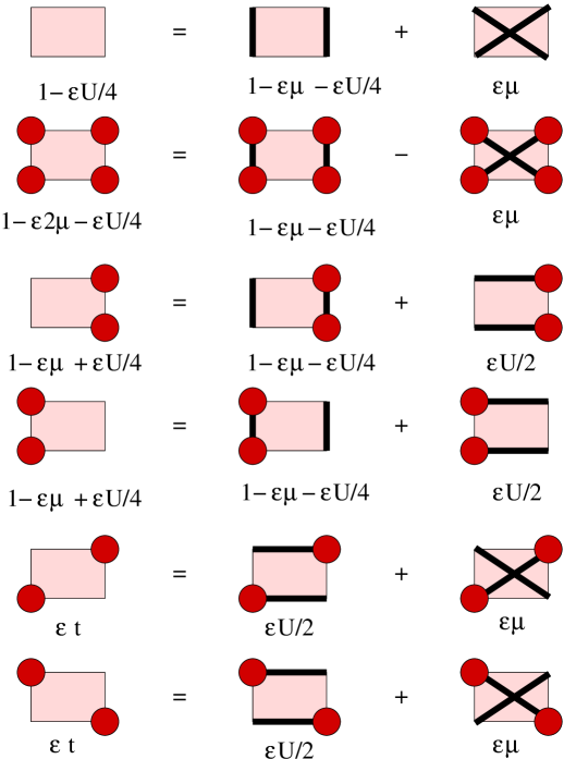
Figure 1: Interaction plaquettes and their weights that contribute to $W[n]$ and $W[n,b]$ so that $Z_{f}$ is preserved. It is assumed that $t=U/2+\mu$.

Figure 1 shows the non-zero transfer matrix elements $[1-\varepsilon h_{x,y}]$ in the occupation number configuration $[n]$ as well as in the extended configuration of occupation numbers and bonds $[n,b]$, such that partition function does not change. A typical configuration of fermion occupation numbers and bonds in one spatial and one temporal direction with $M=4$ is shown in Fig. 2. The shaded regions represent the interaction plaquettes each of which represents a transfer matrix element. The global fermion permutation sign factor for this configuration is $-1$.

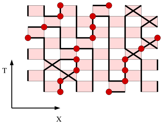
Figure 2: A typical configuration of fermions and bonds.

The significance of the breakup chosen in Fig. 1 is that it yields a model that satisfies properties (a) and (b) of the meron cluster approach. The first property is easily checked by noticing that the magnitude of the weights of the transfer matrix elements depend only on the bonds and not on the fermion occupation numbers. In order to check that the property (b) is also satisfied it is important to find the effect of a cluster flip on $\mbox{Sign}[n,b]$. It can be shown that if

$$\frac{N_{\mbox{side hops}}}{2}+N_{\mbox{cross hop over filled sites}}+N_{\mbox{temporal winding}}$$ (14)

for a cluster is even only then the fermion permutation sign changes when that cluster is flipped. Details of the derivation of this formula can be found in [13]. The formula shows that the cross bonds can in principle induce dependence between clusters. However, the extra local negative sign associated with the fully occupied cross bond in Fig. 1, cancels such dependences. Finally for property (c) to be satisfied one has to either set $\mu=0$ or $U=0$. When $\mu=0$ there are no cross bonds and one can flip all configurations $[n,b]$ to a configuration of staggered spatial fermion occupation which is static in time. This configuration is again guaranteed to be positive [5]. On the other hand when $U=0$ there are no horizontal bonds and one can flip all the configurations $[n,b]$ to a configuration with all sites are empty. This configuration is guaranteed to be positive [6].

5 Fermions with Spin

Fermionic Hamiltonians that are of interest in both nuclear and condensed matter systems, involve internal degrees of freedom like spin and isospin. In order to illustrate how the meron cluster approach can be extended to such systems let us construct a model of fermions with spin which can be viewed as two layers of spin-less fermions. Instead of starting from the Hamilton operator and then constructing the cluster model as we did in the case of spin-less fermions, let us construct the cluster model first. For simplicity, consider models where the bond configuration of Fig. 2 represents a typical configuration on each of the layers. Let the interactions between layers arise due to a constraints on how the bonds in the two layers are related. Fig. 3 shows the allowed bond configurations on each “interaction cube” of a simple interacting model and the magnitude of their weights. This means that every configuration is forced to contain identical clusters in the two layers. In addition, if the allowed fermion occupation numbers on the sites for a given bond configuration satisfy the rules of the previous section (i.e., the occupation numbers of sites connected by vertical and cross bonds must be the same and those connected by horizontal bonds must be opposite) and if all these configurations have the same weight $W[b]$ ( which is the product of the magnitudes of the interaction cube weights specified in Fig. 3) then the model automatically satisfies the property (a) of section 3. Since the clusters live on a single layer we can again use eq. (14) to determine the sign change due to a cluster flip. In order for the cross bonds not to violate property (b), we again associate an extra local negative sign with fully occupied cross bonds on each spin layer. It is easy to check that these restrictions automatically also satisfy property (c) and the cluster model thus becomes solvable with the meron cluster approach.

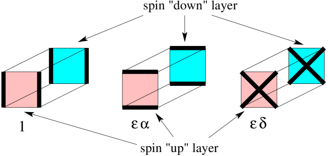
Figure 3: Bond configurations and their weights of an interaction cube for a model with spin.

As before the partition function of the model is given by eq. (11) with $\overline{\mbox{Sign}}[b]$ given by eq. (12). In the present case, the number of clusters $N_{\cal C}$ is always even with $N_{\cal C}/2$ clusters in the spin up layer and an equal number of identical clusters in the spin down layer. When the quantity of eq. (14) is even for any of the clusters then $\overline{\mbox{Sign}}[b]=0$. Such clusters are the meron clusters. When there are no meron clusters in the configuration then $\overline{\mbox{Sign}}[b]=2^{N_{\cal C}}$ since each cluster can have two fermion occupation number configurations associated to it. Retracing the steps of the previous section in the reverse order, we can also determine the associated Hamilton operator. Remembering that $2dM$ is the number of time slices of the lattice and $\varepsilon M=1/T$, it can be shown that the model obtained in the limit $\varepsilon\rightarrow 0$ can be described by the Hamilton operator of eq. (3) with

$$h_{x,y}\;=\;-\delta\left\{[{c_{x,\downarrow}}^{\dagger}c_{y,\downarrow}+{c_{y,\downarrow}}^{\dagger}c_{x,\downarrow}-n_{x,\downarrow}-n_{y,\downarrow}+1]\;\;\;\;\times\right.$$

$$\left.\;\;\;\;\;\;\;\;\;\;\;\;\;\;\;\;\;\;\;\;\;\;\;\;\;[{c_{x,\uparrow}}^{\dagger}c_{y,\uparrow}+{c_{y,\uparrow}}^{\dagger}c_{x,\uparrow}-n_{x,\uparrow}-n_{y,\uparrow}+1]\right\}$$

$$-\alpha\left\{[{c_{x,\downarrow}}^{\dagger}c_{y,\downarrow}+{c_{y,\downarrow}}^{\dagger}c_{x,\downarrow}-2(n_{x,\downarrow}-1/2)(n_{y,\downarrow}-1/2)+1/2]\;\;\;\;\times\right.$$

$$\left.\;\;\;\;\;\;\;\;\;[{c_{x,\uparrow}}^{\dagger}c_{y,\uparrow}+{c_{y,\uparrow}}^{\dagger}c_{x,\uparrow}-2(n_{x,\uparrow}-1/2)(n_{y,\uparrow}-1/2)+1/2]\right\}.$$ (15)

Here the spin up and down fermions are created and annihilated by $c_{x,\uparrow}^{+},c_{x,\downarrow}^{+}$ and $c_{x,\uparrow},c_{x,\downarrow}$ respectively and $n_{x,\uparrow}$ and $n_{x,\downarrow}$ refer to the corresponding number operators.

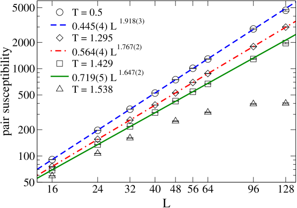
Figure 4: Pair susceptibility as a function of $L$.

The above Hubbard type model has a $U(1)$ fermion number symmetry. In three or more dimensions the breaking of this symmetry leads to superfluidity(or superconductivity when the symmetry is gauged). In two dimensions due to the Mermin Wagner theorem the symmetry cannot break spontaneously and the superfluid transition is driven by the Kosterlitz-Thouless phenomena [14]. It has been difficult to study the predictions of universality in fermionic systems. This is the reason no known calculation exists that confirms the predictions of the Kosterlitz-Thouless phenomena starting from a microscopic fermionic Hamiltonian. The above model for the first time provides an opportunity for studying such a superfluid transition using cluster algorithms. The simplest observable relevant to this transition is the pair susceptibility which can be defined as

$$\chi\;=\;\frac{2T}{ZV}\;\int_{0}^{1/T}\;dt\;{\rm Tr}\left[\;{\rm e}^{-(1/T-t)H}\;p^{+}\;{\rm e}^{-tH}\;p^{-}\;\right]$$ (16)

with $p^{+}=\sum_{x}c_{x,\uparrow}^{\dagger}c_{x,\downarrow}^{\dagger}$ the pair creation and $p^{-}=(p^{+})^{\dagger}$ the pair annihilation operators. In terms of cluster variables the susceptibility is proportional to the sum over the square of the size of certain clusters depending on the number of meron clusters in the configuration. The Kosterlitz-Thouless prediction says that

$$\chi\;\propto\;\left\{\begin{array}[]{cc}L^{2-\eta(T)}&T<T_{c}\cr\mbox{Const.}&T>T_{c}\end{array}\right.$$ (17)

where $\eta(T)$ changes continuously from $0.25$ at $T_{c}$ to $0$ at $T=0$. Figure 4 shows the results for the pair susceptibility as a function of spatial size $L$ in the above model with $\delta=1,\alpha=1,d=2$ and $M=20$. As can be seen, $T=1.538,1.429$ are both above $T_{c}$, although in the latter case lattices of size $L=128$ are necessary to see the saturation. At $T=1.295$ and $T=0.5$ the power law fits are extremely good over the entire range of $L$ with powers $1.767(2)$ and $1.918(3)$. More details can be found in [10].

6 Model Extensions

Although the meron cluster approach helps to find models without sign problems, it is also possible to find cluster models which seem not to satisfy all the properties of the meron cluster approach but still do not suffer from sign problems. For example the model with the Hamilton operator $H=\sum_{x,i}h_{x,x+i}+\sum_{x}h_{x}$, where

$$h_{x}\;=\;U\left(c_{x,\uparrow}-\frac{1}{2}\right)\left(c_{x,\downarrow}-\frac{1}{2}\right)+\mu(n_{x,\uparrow}+n_{x,\downarrow}).$$ (18)

will have the same partition function as eq. (11) except that $\overline{\mbox{Sign}}[b]$ is no longer $2^{N_{\cal C}}$ but is replaced by

$$\prod_{{\cal C}\;\in\;\uparrow\;\mbox{layer}}\left[\mathrm{e}^{(\epsilon/2d)\;\left(-U\;S_{\cal C}/4+\mu\Omega_{\cal C}\right)}+\mathrm{e}^{(\epsilon/2d)\;\left(-U\;S_{\cal C}/4-\mu\Omega_{\cal C}\right)}\right]\;\pm\;2\;\mathrm{e}^{(\epsilon/2d)\;U\;S_{\cal C}/4},$$ (19)

where $S_{{\cal C}}$ is the size of the cluster ${\cal C}$ and $\Omega_{\cal C}$ is $2dM$ times the cluster’s temporal winding number. The negative sign should be taken for a meron cluster. This factor is obviously positive for any $\mu$ if $U<0$. Interestingly, it is also positive for $\mu<U/2$ if $\delta=0$ and $U>0$ since then meron clusters always come in pairs. The proof also uses the fact that for all clusters $S_{\cal C}\geq\Omega_{\cal C}$. Thus we have found a repulsive Hubbard type model which does not suffer from a sign problem when formulated in the cluster approach for at least a limited range of chemical potentials.

7 Conclusions

We have sketched how a variety of fermionic partition functions can be written as a sum over cluster configurations with positive definite weights. The three properties of the meron cluster approach discussed in section 3 help find such models. However, it is possible to relax these properties and find extensions in certain cases. One drawback of this approach is that the new models possess a complicated Hamilton operator. On the other hand, given the numerical efficiency of the algorithms that can be constructed for them it may still be useful to study these models. For example this approach has led to the first precise confirmation of universality arguments in fermionic systems [7-10]. Other applications in condensed matter and nuclear physics are being explored.

8 Acknowledgment

I would like to thank J. C. Osborn and U.-J. Wiese for their collaboration. This work is supported in part by funds provided by US Department of Energy grant DE-FG02-96ER40945 and the National Science Foundation grant DMR-0103003.

References

- [1] S. Duane and J. Kogut, Phys. Rev. Lett. 55 (1985) 2774.
- [2] M. Lüscher, Nucl. Phys. B418 (1994) 637.
- [3] S. R. White et. al., Phys. Rev. B38 (1988) 11695.
- [4] S. Zhang et. al., Phys. Rev. Lett 74 (1995) 3652.
- [5] S. Chandrasekharan and U.-J. Wiese, Phys. Rev. Lett. 83, 3116 (1999).
- [6] S. Chandrasekharan, Nucl. Phys. (Proc. Suppl.) 83-84, 774 (2000).
- [7] S. Chandrasekharan et al., Nucl. Phys. B576, 481 (2000).
- [8] S. Chandrasekharan and J. C. Osborn, Phys. Lett. B496, 122 (2000).
- [9] J. Cox and K. Holland, Nucl. Phys. B583, 331 (2000).
- [10] S. Chandrasekharan and J. C. Osborn, cond-mat/0109424.
- [11] S. Chandrasekharan, et. al., in preparation.
- [12] U.-J. Wiese, Phys. Lett. B311 (1993) 235.
- [13] S. Chandrasekharan, Springer Proceedings of Physics, 86 (2000) 28.
- [14] J. M. Kosterlitz and D. J. Thouless, J. Phys. C6, 1181 (1973).