Chirally improved Dirac operators: Studying the sensitivity to topological excitations for zero and finite temperature

Abstract

We discuss the construction and properties of an approximate solution of the Ginsparg-Wilson equation, the so-called chirally improved lattice Dirac operator. In particular we study the behavior of its eigenmodes in smooth instanton backgrounds as well as for thermalized gauge configurations on both sides of the QCD phase transition. We compare with results from other Dirac operators including the overlap operator. The results support the picture of chiral symmetry breaking being closely related to instantons.

1 Motivation and introduction

During the last three years it has been realized that the Ginsparg-Wilson relation [1] is the key to chirally symmetric fermions on the lattice. However, the overlap operator [2] which exactly solves the Ginsparg-Wilson equation is numerically very expensive. For many applications an alternative to an exact solution is an approximate Ginsparg-Wilson Dirac operator, such as a finite parametrization of the perfect action [3] or the recently proposed chirally improved Dirac operator [4]. The latter results from a systematic expansion of a solution of the Ginsparg-Wilson equation.

In this contribution we report on our results for the eigenvectors and eigenvalues of the chirally improved Dirac operator, using smooth instanton backgrounds as well as thermalized (quenched) gauge configurations on both sides of the QCD phase transition. These studies serve two purposes: Firstly, they allow to obtain a sound understanding of the properties of the chirally improved Dirac operator. In particular we also compare our results to calculations done with the overlap operator in order to understand the effects of small violations of chirality. Secondly, the analysis of the eigenmodes provides insights into the nature of the QCD vacuum, since the eigenvectors couple to localized objects in the underlying gauge field such as instantons or instanton anti-instanton molecules.

2 Remarks on the construction of the lattice Dirac operators

Chirally improved operator: In [4] we suggested an expansion of the lattice Dirac operator $D$ in terms of a systematic series of simple hopping terms, connecting sites along paths of arbitrary length and allowing for all elements of the Clifford algebra. For the ansatz one respects all standard translational and rotational symmetries of the lattice Dirac operator as well as invariance under C and P and $\gamma_{5}$-hermiticity. We insert that formal series into

$$E\equiv-D-D^{\dagger}+D^{\dagger}\,D\;.$$ (1)

Finding a solution to the Ginsparg-Wilson equation [1] amounts to solving for $E=0$. The product $D^{\dagger}\,D$ is again constructed algebraically, leading to terms involving Clifford algebra elements and paths corresponding to ordered products of gauge link variables.

$E$ is an infinite series of terms that are linear and quadratic in the coupling coefficients of the Dirac operator multiplying the path terms. Independent terms have to vanish and thus we obtain a system of coupled equations quadratic in the (unknown) coupling constants. We truncate the ansatz for $D$ and the series for $E$ at paths of length 4. Whereas the complete series would lead to an exact solution of the Ginsparg-Wilson equation, the solution now will only be approximate and it remains to be studied, how good this approximation is.

In solving the set of equations there is much freedom. In order to partially remedy the approximation we introduce two more conditions (and parameters) such that the boundary condition for a massless Dirac operator

$$\hat{D}(p)\equiv i\not p+{\cal O}(p^{2})\;,$$ (2)

is satisfied at a given value of the gauge coupling. The solution we study here has 19 terms and values of the coefficients are listed in the appendix of [5]. It is ultralocal with non-vanishing couplings only for $|x-y|\leq\sqrt{5}$ decreasing exponentially in size.

Exact solutions to the Ginsparg-Wilson equation ($E=0$) have eigenvalues on a unit circle with center 1 in the complex plane. It turned out that our solution, defining a chirally improved Dirac operator, has eigenvalues, that are very close to the unit circle in particular for the small eigenvalue region, which is most relevant for the infrared behavior.

Overlap operator: Below we compare the properties of the sector with small eigenvalues (complex or real) of the introduced chirally improved operator with those of an overlap operator [2] which has the form

$$D_{ov}=1-Z\quad\textrm{with}\quad Z\equiv\gamma_{5}\,\mathop{\mathrm{sign}}\nolimits(H)\;,$$ (3)

where $H$ is related to the hermitian Dirac operator. This is constructed from an arbitrary Dirac operator $D_{0}$ (e.g. the Wilson operator),

$$H=\gamma_{5}\,(s-D_{0})\;,$$ (4)

and $s$ is a parameter which may be adjusted in order to minimize the probability for zero modes of $H$. In case $D_{0}$ is already an overlap operator one reproduces $D_{ov}=D_{0}$ for $s=1$ because $\mathop{\mathrm{sign}}\nolimits\left(\mathop{\mathrm{sign}}\nolimits(H)\right)=\mathop{\mathrm{sign}}\nolimits(H)$.

The sign-function may be defined through the spectral representation

$$\mathop{\mathrm{sign}}\nolimits H=\sum_{i}\,\mathop{\mathrm{sign}}\nolimits\lambda_{i}\,|i\rangle\langle i|\;,$$ (5)

($|i\rangle$ denote the eigenvectors) but in practical computations this definition cannot be used for realistic QCD Dirac operators, which for $L^{4}$ lattices have dimension $\mathcal{O}(10^{5}-10^{6})$ ($\sim n_{color}\cdot n_{Dirac}\cdot L^{4}$). Note that in the subsequent applications the operator has to be applied many times, since it may be entering a diagonalization or a conjugate gradient inversion tool. One therefore relies on the relation

$$\mathop{\mathrm{sign}}\nolimits(H)=\frac{H}{\sqrt{H^{2}}}$$ (6)

and approximates the inverse square by some method. In our computations [6] we follow the methods discussed in [7, 8]. One approximates the inverse square root by a Chebychev polynomial, which has exponential convergence in $[\epsilon,1]$, where $\epsilon$ (and thus the order of the polynomial) depends on the ratio of smallest to largest eigenvalue of $H^{2}$. Clenshaw’s recurrence formula provides further numerical stability.

Depending on the input Dirac operator $D_{0}$ the rate of convergence may be quite unfavorable. Although one may adjust $s$ it turns out that particular simple operators like the Wilson Dirac operator eventually will give rise to several small eigenvalues of $H^{2}$. Technically, one then proceeds as follows: One determines the subspace of e.g. the lowest 20 eigenmodes of $H^{2}$ and computes the inverse square separately for the subspace (using the spectral representation) and the reduced operator (with polynomial approximation). For this approach it is important to determine the subspace with high accuracy (we request 12 digits).

In our study we need to diagonalize not only the hermitian matrix $H$ but, for the later analysis, also $D_{ov}$ and the chirally improved operator. All diagonalizations have been done with the Arnoldi method [9].

CPU-time comparison: The central element of the diagonalization (and conjugate gradient methods) is the multiplication of the Dirac operator with a vector. For the consideration of the computational effort we disregard the startup time for initialization of the operator. Comparing the CPU-time in units of the time used for the Wilson Dirac operator we find that the chirally improved operator needs 24 units and the overlap operator (with Wilson input) typically needs $300\pm 100$ units (always with 12 digits accuracy for the matrix norm $||H^{2}-1||$). These are the results for lattice size $12^{4}$, but they are not significantly different for $8^{4}$ or $16^{4}$.

As mentioned, whenever $(1-D_{0})$ is already an overlap operator, one finds $D_{ov}=D_{0}$. We are interested in the case when $(1-D_{0})$ is close to, but not quite an overlap operator. Such an operator might accelerate the convergence in the construction of the overlap operator, since the convergence of the polynomial approximation depends crucially on the smallest eigenvalue of $H^{2}$. It is therefore of high practical importance, whether $H$ will have eigenvalues close to zero. A Dirac operator $D_{0}$ used as input to the construction of $H$ may produce such small eigenvalues. Physically they are related to the appearance or disappearance of an instanton. Different Dirac operators will differ in their sensitivity to “identify” such structures in the gauge configuration.

When using the chirally improved operator – in comparison to using the Wilson Dirac operator – as starting point we need typically a factor 2 less matrix-vector multiplications ($75\pm 25$ terms of the Chebychev series for $12^{4}$ or $16^{4}$ lattices). One reason that this improvement factor is not higher may lie in the removal of the small eigenmode subspace, which is relatively more efficient for the “bad” Wilson operator used as input to the overlap construction. Another reason may be that the series approximation forces all eigenvalues to the unit circle; since the chirally improved operator has its large eigenvalues not as close to the circle as the small ones, one has to pay the price with longer polynomials.

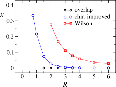
Figure 1: Position $x$ of the real eigenvalue (the would-be zero mode) of different lattice Dirac operators as a function of the radius $R$ of the underlying instanton configuration.

3 Small eigenvalues and instantons

For an instanton in the continuum it is known that the Dirac operator has a zero mode. On the lattice only an exact solution of the Ginsparg-Wilson equation will display an eigenvalue which vanishes exactly. An approximate Ginsparg-Wilson Dirac operator will then have a small real eigenvalue. Typically the size of the real part will increase as one shrinks the radius of the underlying instanton. The rate at which the real eigenvalue moves away from the origin is a measure for the quality of the approximate solution of the Ginsparg-Wilson equation. A good approximation will keep the eigenvalue near zero also for relatively small instantons. In order to implement this test of the would-be zero modes we use instantons with several values of the radius $R$ discretized on the lattice following the method described in [10, 6].

Fig. 1 shows the position $x$ of the real eigenvalue (the would-be zero mode) of different Dirac operators as a function of the radius $R$ of the underlying instanton. We show the results computed on $16^{4}$ lattices for the chirally improved operator (circles), the Wilson operator (squares), and the overlap operator (diamonds). The latter, since it is an exact solution of the Ginsparg-Wilson equation, has an exact zero mode. It is, however, interesting to see that the overlap operator can trace the instanton only down to a radius $R=1.5$. The Wilson operator has an eigenvalue which very quickly departs from zero as $R$ is decreased. The chirally improved operator keeps the real eigenvalue fairly close to 0 even for relatively small instantons and only for $R\leq 2$ the deviation becomes significant.

For practical applications of the chirally improved Dirac operator, the question is whether also in a gauge configuration with quantum fluctuations the real eigenmodes lie close to the origin. In order to test this property, we computed histograms for the probability distribution of the real eigenvalues. The gauge fields were generated in a quenched simulation, using the tadpole improved Lüscher-Weisz action [11]. The histograms were computed on $16^{4}$ lattices at values of $\beta_{1}=$ 8.10, 8.30 and 8.45 using 200 configurations for each $\beta_{1}$. The corresponding values of the couplings $\beta_{2}$ and $\beta_{3}$ of the gauge action can be found in [12]. There we obtained for the lattice spacing $a$ the values 0.127 fm, 0.107 fm, and 0.1 fm for $\beta_{1}=$ 8.10, 8.30, and 8.45, respectively.

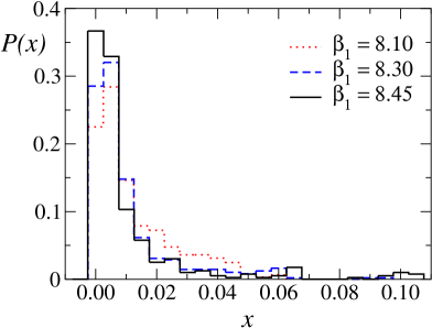
Figure 2: Probability distribution of the position $x$ of the real eigenvalues of the chirally improved Dirac operator. The data were computed on $16^{4}$ lattices at values of $\beta_{1}=8.10,8.30$ and 8.45 using 200 configurations for each $\beta_{1}$.

From Fig. 2 it is obvious that the eigenvalues are concentrated near the origin. The tail of the distribution decays very quickly and extends almost exclusively towards values $x>0$. Both these features are highly welcome: The narrow width of the distribution lets one hope for only a very small additive renormalization of the quark mass. The fact that the distribution does not extend to values $x<0$ implies furthermore that exceptional configurations (which spoil the computation of the propagator) are suppressed effectively.

4 Localization properties of zero modes

We now analyze the eigenvectors with real eigenvalues, i.e. the modes which correspond to the zero modes in the continuum. For a continuum instanton the zero modes are known to be localized at the same position as the instanton. This property also holds for thermalized configurations on the lattice [13]. The eigenmodes provide an efficient filter for the excitations of the QCD vacuum as seen by the Dirac operator.

To study the eigenvectors we define the scalar density $p_{0}(x)$. Let $\psi(x)_{c}$ be an eigenvector of the Dirac operator with $x$ denoting the lattice point while $c$ is the color index. A gauge invariant density $p_{\sigma}(x)$ is defined as

$$p_{\sigma}(x)=\sum_{c}\psi(x)_{c}^{*}\,\Gamma_{\sigma}\,\psi(x)_{c}\;.$$ (7)

(Here $\Gamma_{0}=\mathbf{1}$, $\Gamma_{5}=\gamma_{5}$; the sum over Dirac indices is implied.) In the last section we have seen that the continuum zero modes correspond to eigenvectors of the lattice Dirac operator with eigenvalue zero (overlap operator) or small real eigenvalue (chirally improved operator, Wilson operator). An interesting question is, to which extent the eigenvectors are different for different lattice Dirac operators.

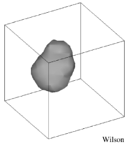
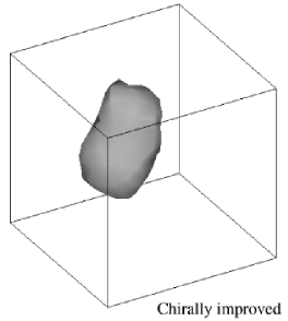
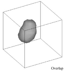
Figure 3: Comparison of iso-surfaces (for a given time-slice) of the scalar density for the zero-mode of different Dirac operators. We show the density for the Wilson operator (top), the chirally improved operator (middle), and the overlap operator (bottom).

In Fig. 3 we compare iso-surfaces of the scalar density for the zero-mode of different Dirac operators on the same gauge configuration ($12^{4}$ lattice at $\beta_{1}=8.45$). All three operators see the same localized instanton. Only the details vary slightly as can be seen by the different fluctuations around the core.

An interesting effect was observed for small instantons in [6] where we compared the localization of the zero mode for the smooth instantons discussed above for different lattice Dirac operators. It was found that for instantons with radius smaller than 3 in lattice units, the overlap operator has a zero mode which is less localized than in the case of a continuum instanton. Since the other two operators (chirally improved, Wilson) do not display such a blowing up of zero modes we attribute this effect to the rather big size of the overlap operator. As opposed to the other two operators the overlap operator is not ultra-local, i.e. $|D_{ov}(x,y)|$ decays exponentially with $|x-y|$ but does not vanish exactly. Objects smaller than the typical size of the overlap operator thus can no longer be resolved. We estimate [6] that at typical lattice spacings of $a\sim$ 0.1 fm this effect sets in at about 0.3 fm.

For further study we introduce the so-called inverse participation ratio, a convenient measure of the localization widely used in solid state physics. Due to the normalization of the eigenmodes we have $\sum_{x}\,p_{0}(x)=1$. The inverse participation ratio is then defined as

$$I\;=\;V\sum_{x}\,p_{0}(x)^{2}\;,$$ (8)

where $V$ is the volume of the lattice. An alternative observable for localization, based on the self correlation of the scalar density $p_{0}(x)$ was analyzed in [14].

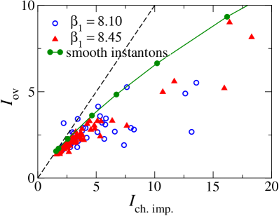
Figure 4: Comparing the localization of the zero modes of the chirally improved operator and the overlap operator.

In Fig. 4 we show a scatter plot of the inverse participation ratio for zero modes of the overlap operator $I_{ov}$ plotted as a function of the inverse participation ratio of the corresponding modes of the chirally improved operator $I_{ch.~{}imp.}$. The data were computed on $12^{4}$ lattices using 200 configurations at $\beta_{1}=8.10$ (circles), and $\beta_{1}=8.45$ (filled triangles). The full curve with filled circles is the result for the smooth artificial instantons. The dashed line is a straight line with slope 1. If both operators would see the same localization for the zero modes, all data points would be located on this line. However, obviously this is not the case. Except for a single data point, all data are below this line. This means that the overlap operator systematically produces zero modes with smaller localization when compared to the chirally improved operator; this trend becomes stronger for more localized states.

5 Analysis of the near-zero modes

So far we have concentrated on analyzing the eigenvectors with real eigenvalues, i.e. the would-be zero modes. However, also the eigenvectors with small but complex eigenvalues, the so-called near-zero modes, play an important role in QCD phenomenology. In particular the eigenvalue density $\rho(\lambda)$ near at the origin is related to the chiral condensate through the Banks-Casher formula [15],

$$\langle\overline{\psi}\psi\rangle\;=\;-\pi\lim_{\lambda\to 0}\lim_{V\to\infty}\rho(\lambda)V^{-1}\;.$$ (9)

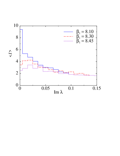
Figure 5: Histograms of the inverse participation ratio for eigenvectors as a function of the imaginary part of the corresponding eigenvalue.

According to the instanton liquid picture of chiral symmetry breaking [16], the near-zero modes come from weakly interacting instantons and anti-instantons. The corresponding eigenvectors are expected to be still quite localized, since they correspond to interacting “lumps” which still resemble instantons or anti-instantons. These predictions may be tested in an ab-initio calculation on the lattice. Again we use the inverse participation ratio defined in Eq. (8) to study the localization of these modes. An interesting question is how the localization of eigenvectors varies as a function of the eigenvalue.

In Fig. 5 we show a histogram of the inverse participation ratio for eigenvectors as a function of the imaginary part of the corresponding eigenvalues. The data were computed on $16^{4}$ lattices at values of $\beta_{1}=8.10,8.30$ and 8.45 using 200 configurations for each $\beta_{1}$. It is obvious that the most localized states have eigenvalues near the origin. Such large values are expected for weakly interacting instantons and anti-instantons. As $\textrm{Im\,}\lambda$ is increased, the localization decreases. The corresponding modes do no longer feel distinguished topological lumps but become dominated by quantum fluctuations.

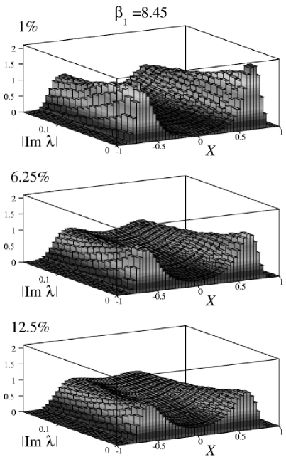
Figure 6: Local chirality of eigenvectors as a function of $\textrm{Im\,}\lambda$ of the corresponding eigenvalues. We use cuts of 1% (top) 6.25% (middle) and 12.5 % (bottom) for the number of supporting points.

An interesting observable was suggested by Horvath et al. in [17]. Their local chirality variable was subsequently studied by several other groups in [18, 5, 12]. The underlying idea is to test whether the near-zero modes are locally chiral, i.e. left-handed for lattice points near the instanton peak of the density and right-handed near the anti-instanton peak. The construction starts with defining left- and right-handed densities $p_{\pm}(x)$,

$$p_{\pm}(x)=\frac{1}{2}\left(p_{0}(x)\pm p_{5}(x)\right)\;,$$ (10)

i.e. the density (7) projected on positive and negative chirality. A mode dominated by instantons and anti-instantons is expected to have $p_{+}(x)>0$ and $p_{-}(x)=0$ for lattice points $x$ near the instanton peak and vice versa for $x$ near an anti-instanton peak. Thus the ratio $p_{+}(x)/p_{-}(x)$ should be large for $x$ close to an instanton peak and small for all $x$ close to an anti-instanton peak. In a final step Horvath et al. map the positive real values of this ratio onto the interval between $-1$ and $+1$ using the transformation

$$X(x)\;=\;\frac{4}{\pi}\;\mbox{arctan}\,\left(\sqrt{\frac{p_{+}(x)}{p_{-}(x)}}\right)\;-\;1\;.$$ (11)

In order to suppress the quantum fluctuations one evaluates $X(x)$ only for $x$ near instanton or anti-instanton peaks, i.e. for $x$ near the maxima of the scalar density $p_{0}(x)$. We computed our results using cutoffs of 1%, 6.25% and 12.5% for the number of lattice points $x$ (ordered according to $p_{0}(x)$) and averaged over $X(x)$. On the gauge field ensemble the local chirality variable is expected to show a double peak structure only for instanton dominance.

In Fig. 6 we show the local chirality of the near-zero modes as a function of the imaginary part of their eigenvalues. The data were computed from 200 configurations on $16^{4}$ lattices at $\beta_{1}=8.45$. When using a cut of 1% on the number of supporting lattice points (top plot) we find the best signal while for cuts of 6.25% (middle plot) and 12.5% (bottom plot) the signal becomes weaker due to quantum fluctuations. Furthermore it is obvious for all three plots that the strongest signal for local chirality is found for the eigenvectors with eigenvalues closest to the origin. For larger values of $|\textrm{Im\,}\lambda|$ the signal of local chirality for the corresponding eigenvectors weakens and the mode becomes dominated by quantum fluctuations.

Figure 7: The inverse participation ratio as a function of the imaginary part of the corresponding eigenvalue. These data were computed at $\beta_{1}=8.45$ where (with time extent 6) the theory is in the deconfined phase. In the subsample used here the expectation value of the Polyakov loop $\langle L\rangle$ is close to real.

6 The near-zero modes at finite temperature

Let us now discuss what happens to instantons at the QCD phase transition. At the critical temperature $T_{c}$ the theory enters the deconfined phase and chiral symmetry is restored. The spectrum develops a gap (see e.g. [5] for a plot of typical spectra) and the density of eigenvalues is zero near the origin. According to the Banks-Casher formula (9) this gap in the spectral density amounts to a vanishing chiral condensate.

The topological charge does not vanish abruptly at $T_{c}$ and topological objects are observed also for $T>T_{c}$. Thus the liquid of weakly interacting instantons responsible for chiral symmetry breaking at $T<T_{c}$ must undergo some change in its structure as the temperature is increased above $T_{c}$. It may be expected that above $T_{c}$ instead of interacting weakly, instantons and anti-instantons form tightly bound molecules [16]. This prediction from instanton models can be tested on the lattice (compare [19] for a similar study using the staggered Dirac operator).

In Fig. 7 we show the inverse participation ratio as a function of the imaginary part of the corresponding eigenvalue, as in Fig. 5, but now for finite temperature. In particular we show the results for configurations where the Polyakov loop $\langle L\rangle$ is in its real branch, which is the domain of the Polyakov loop value for the full, unquenched theory. For the equivalent plot with complex Polyakov loop see [5]. Due to the spectral gap in the deconfined phase, there are no near-zero modes and the graph has support for $|\textrm{Im\,}\lambda|>0.15$. One finds that now the most localized states are near the edge of the spectrum. Localization decreases quickly as $|\textrm{Im\,}\lambda|$ is increased and the mode becomes a bulk mode dominated by quantum fluctuations. The inverse participation ratio, however, provides only information on the localization of the modes and does not test for other properties such as local chirality. Thus it makes sense to repeat last section’s study of Horvath et al.’s local chirality variable for $T>T_{c}$.

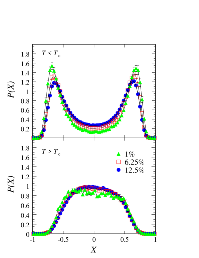
Figure 8: Comparison of the local chirality of the (complex) near-zero modes for $T<T_{c}$ (top) and $T>T_{c}$ (bottom).

In Fig. 8 we compare the local chirality of the near-zero modes for an ensemble at $T<T_{c}$ (top plot, $6\times 20^{3}$ lattices, 400 configurations at $\beta_{1}=8.10$) with an ensemble at $T>T_{c}$ (bottom plot, $6\times 20^{3}$ lattices, 147 configurations with real branch Polyakov loop at $\beta_{1}=8.45$). The plots were computed using only the eigenvectors with $|\textrm{Im\,}\lambda|$ less than some cut corresponding to roughly the 4 eigenvalues closest to the origin, respectively the edge of the spectrum. Zero modes were left out. For $T<T_{c}$ we find a very pronounced double peak structure, i.e. a strong signal for local chirality. At $T>T_{c}$ the double peak structure is gone and we do not observe local chirality in the eigenmodes. It is obvious that the weakly interacting instantons and anti-instantons undergo a drastic change as $T$ increases above $T_{c}$. The resulting states are still localized (see Fig. 7) but the local chirality present for weakly interacting topological excitations has vanished, probably due to the formation of tightly bound molecules.

Acknowledgements: We thank the Leibniz Rechenzentrum in Munich for computer time on the Hitachi SR8000 and their operating team for support and training. C. Gattringer and C.B. Lang thank the DOE’s Institute of Nuclear Theory at the University of Washington for its hospitality and the DOE for partial support during the completion of this work. We have profited considerably from discussion with Pierre van Baal, Tom DeGrand, Stefan Dürr, Peter Hasenfratz, Ivan Hip and Ferenc Niedermayer.

References

- [1] P.H. Ginsparg and K.G. Wilson, Phys. Rev. D 25 (1982) 2649.
- [2] R. Narayanan and H. Neuberger, Phys. Lett. B 302 (1993) 62, Nucl. Phys. B 443 (1995) 305.
- [3] P. Hasenfratz, Nucl. Phys. B (Proc. Suppl.) 63 (1998) 53; P. Hasenfratz, Nucl. Phys. B 525 (1998) 401; P. Hasenfratz, V. Laliena and F. Niedermayer, Phys. Lett. B 427 (1998) 353; P. Hasenfratz, S. Hauswirth, K. Holland, Th. Jörg, F. Niedermayer and U. Wenger, Int. J. Mod. Phys. C12 (2001) 691; P. Hasenfratz, S. Hauswirth, K. Holland, Th. Jörg and F. Niedermayer, hep-lat/0109004, hep-lat/0109007.
- [4] C. Gattringer, Phys. Rev. D 63 (2001) 114501; C. Gattringer, I. Hip and C.B. Lang, Nucl. Phys. B597 (2001) 451; C. Gattringer and I. Hip, Phys. Lett. B 480 (2000) 112.
- [5] C. Gattringer, M. Göckeler, P.E.L. Rakow, S. Schaefer and A. Schäfer, hep-lat/0105023.
- [6] C. Gattringer, M. Göckeler, C.B. Lang, P.E.L. Rakow and A. Schäfer, hep-lat/0108001.
- [7] P. Hernández, K. Jansen, and M. Lüscher, Nucl. Phys. B 552 (1999) 363; P. Hernandez, K. Jansen, and L. Lellouch, hep-lat/0001008, 2000.
- [8] B. Bunk, Nucl. Phys. B (Proc. Suppl.) 63 (1998) 952.
- [9] D.C. Sorensen, SIAM J. Matrix Anal. Appl. 13 (1992) 357; R. B. Lehoucq, D.C. Sorensen and C. Yang, ARPACK User’s Guide, SIAM, New York, 1998.
- [10] I.A. Fox, M.L. Laursen, G. Schierholz, J.P. Gilchrist and M. Göckeler, Phys. Lett. B 158 (1985) 332.
- [11] M. Lüscher and P. Weisz, Commun. Math. Phys. 97 (1985) 59; Erratum: 98 (1985) 433; G. Curci, P. Menotti and G. Paffuti, Phys. Lett. B 130 (1983) 205; Erratum: B 135 (1984) 516; M. Alford, W. Dimm, G.P. Lepage, G. Hockney and P.B. Mackenzie, Phys. Lett. B 361 (1995) 87.
- [12] C. Gattringer, M. Göckeler, P.E.L. Rakow, S. Schaefer and A. Schäfer, hep-lat/0107016 (Nucl. Phys. B, in print).
- [13] M.C. Chu, J.M. Grandy, S. Huang and J.W. Negele, Phys. Rev. D 49 (1994) 6039.
- [14] T. DeGrand and A. Hasenfratz, Phys. Rev. D 64 (2001) 034512.
- [15] T. Banks and A. Casher, Nucl. Phys. B 169 (1980) 103.
- [16] T. Schäfer and E.V. Shuryak, Rev. Mod. Phys. 70 (1998) 323; D. Diakonov, Talk given at International School of Physics, ’Enrico Fermi’, Course 80: Selected Topics in Nonperturbative QCD, Varenna, Italy, 1995, hep-ph/9602375.
- [17] I. Horváth, N. Isgur, J. McCune and H.B. Thacker, hep-lat/0102003.
- [18] T. DeGrand and A. Hasenfratz, hep-lat/0103002; I. Hip, Th. Lippert, H. Neff, K. Schilling and W. Schroers, hep-lat/0105001; R.G. Edwards and U.M. Heller, hep-lat/0105004; T. Blum, N. Christ, C. Cristian, C. Dawson, X.Liao, G. Liu, R. Mawhinney, L. Wu and Y. Zhestkov, hep-lat/0105006.
- [19] M. Göckeler, P.E.L. Rakow, A. Schäfer, W. Söldner and T. Wettig, Phys. Rev. Lett. 87 (2001) 042001.