Diquark condensation in dense adjoint matter

Abstract

We study SU(2) lattice gauge theory at non-zero chemical potential with one staggered quark flavor in the adjoint representation. In this model the fermion determinant, although real, can be both positive and negative. We have performed numerical simulations using both hybrid Monte Carlo and two-step multibosonic algorithms, the latter being capable of exploring sectors with either determinant sign. We find that the positive determinant sector behaves like a two-flavor theory, with the chiral condensate rotating into a two-flavor diquark condensate for $\mu>m_{\pi}/2$, implying a superfluid ground state. Good agreement is found with analytical predictions made using chiral perturbation theory. In the ‘full’ model there is no sign of either onset of baryon density or diquark condensation for the range of chemical potentials we have considered. The impact of the sign problem has prevented us from exploring the true onset transition and the mode of diquark condensation, if any, for this model.

1 Introduction

In recent years, significant progress has been made in understanding the phase diagram of QCD at non-zero baryon chemical potential (for reviews, see Rajagopal:2000wf ; Alford:2001dt ). On the basis of numerous model calculations, it is now believed that the ground state of QCD at high density is characterised by a diquark condensate which spontaneously breaks gauge and/or baryon number symmetries Bailin:1984bm ; Alford:1997zt ; Rapp:1998zu ; Alford:1998mk . However, although the results appear to be qualitatively independent of the specific model and approximation employed, little can be said quantitatively due to the lack of a first-principles, nonperturbative method that can access the relevant regions of the phase diagram.

Lattice QCD, which would be such a method, fails because the Euclidean-space fermion determinant becomes complex when a chemical potential is included, so standard algorithms cannot be applied. However, it is possible to study QCD-like theories where the fermion determinant remains real even at non-zero $\mu$. These theories can be used as testbeds to examine the validity of the models used to study real QCD, as well as directly to improve our understanding of phenomena such as diquark condensation and phase transitions in dense matter. Examples of such theories are two-color QCD, QCD with adjoint quarks or at non-zero isospin chemical potential Son:2000xc , and the Nambu–Jona-Lasinio model Hands:1998kk ; Lucini:2000 . A further point of interest is that chiral perturbation theory ($\chi$PT) may also be applied to many of these theories Kogut:1999iv ; Kogut:2000ek ; Splittorff:2000mm .

Two-color QCD with a baryon chemical potential has been an object of study for lattice theorists for many years Nakamura:1984 ; Dagotto:1987 ; klatke:1990 ; there have recently been a number of simulations with quarks in the fundamental representation Morrison:1998ud ; Hands:1999md ; Aloisio:2000if ; Bittner:2000rf ; Liu:2000in ; Muroya:2000qp ; Kogut:2001na ; Kogut:2001if . Here we will be studying two-color QCD with staggered fermions in the adjoint representation. The symmetries and conjectured phase diagram of this model have been presented in a previous paper Hands:2000ei ; here we summarise the main features:

• For an odd number of staggered flavors $N$, the fermion determinant may be negative. This means that this model still has a sign problem, which may make simulations at large $\mu$ difficult.

• At $m=\mu=0$ the $\operatorname{U}(N)\times\operatorname{U}(N)$ flavor symmetry is enhanced to a $\operatorname{U}(2N)$ symmetry which relates quarks to antiquarks. This symmetry is broken by the chiral condensate to $\mathrm{Sp}(2N)$, leaving $N(2N-1)$ massless Goldstone modes, which become degenerate pseudo-Goldstone states for $m\neq 0$.

• When $N\geq 2$ these pseudo-Goldstone states include gauge invariant scalar diquarks, which are thus degenerate with the pion at $\mu=0$. These models can be studied for $\mu\not=0$ by $\chi$PT Kogut:2000ek , the main result being that for $\mu>m_{\pi}/2$ the chiral condensate rotates into a diquark condensate (the two being related by a $\operatorname{U}(2N)$ rotation) while the baryon density increases from zero. For $N=2$ the diquark operator which condenses is

  $$qq_{\bf 3}=\frac{i}{2}\left[\chi^{p\,tr}(x)\varepsilon^{pq}\chi^{q}(x)+\bar{\chi}^{p}(x)\varepsilon^{pq}\bar{\chi}^{q\,tr}(x)\right],$$ (1)

  where $p,q=1,2$ are explicit flavor indices and $\varepsilon$ the antisymmetric tensor.

• The model with $N=1$ is not expected to contain any diquark pseudo-Goldstones and is not accessible to $\chi$PT. We expect an onset transition as some $\mu_{o}\approx m_{b}/n_{q}>m_{\pi}/2$, where $m_{b}$ is the mass of the lightest baryon and $n_{q}$ its baryon charge.

• For $N=1$ the operator (1) is forbidden by the Exclusion Principle; there is, however, a possibility of a gauge non-singlet, and hence color superconducting, diquark condensate at large chemical potential:

  $$qq_{sc}^{i}=\frac{1}{2}\left[\chi^{tr}(x)t^{i}\chi(x)+\bar{\chi}(x)t^{i}\bar{\chi}^{tr}(x)\right]\,,$$ (2)

  where $t^{i}$ is a group generator in the adjoint representation. Since $qq_{sc}^{i}$ also transforms in the adjoint representation of the gauge group, the difference between the sum of the Casimirs of the constituents and that of the composite is positive, and hence the interaction due to one-gluon exchange is attractive in this channel.

The indication in Hands:2000ei  (and the update in Hands:2000yh ) is that the positive determinant sector of the $N=1$ model behaves like the model with $N=2$. Ignoring the determinant sign has the effect of introducing extra ‘conjugate quark’ degrees of freedom $q^{c}$, which carry positive baryon charge but transform in the conjugate representation of the gauge group Stephanov:1996ki . In three-color QCD this approximation leads to unphysical light $qq^{c}$ states which distort the physics of $\mu\not=0$ beyond recognition. In two-color QCD the effect is more subtle; generically the physical spectrum contains $qq^{c}$ states unless expressly forbidden by the Exclusion Principle. For models with staggered lattice fermions this is the case for $N=1$ adjoint flavor Hands:2000ei . In principle, therefore, by simulating this model we may get information about two ‘physical’ models for the price of one; $N=1$ by taking account of the determinant sign, and $N=2$ by ignoring it. The present paper aims to strengthen the evidence for this scenario. As discussed in Hands:2000ei , for $N=1$ staggered adjoint quarks, corresponding to four physical flavors, the continuum limit is problematic since the model is not asymptotically free. Our primary interest remains in studying a strongly interacting model with the potential to show superconducting behaviour regardless of these issues.

The remainder of the article is organised as follows. In section 2 we study the performance of the two-step multibosonic algorithm. In section 3 we present our results. In sec. 3.2 we study the chiral condensate, fermion density, and pion mass and susceptibilities, and demonstrate the different physical behaviour of the positive determinant sector and the full theory. In sec. 3.3 we study pure gauge observables and the effect of Pauli blocking in the positive determinant sector. Secs. 2, 3.2 and 3.3 all build on the results of Hands:2000ei . In sec. 3.4 we present new results for diquark condensation, in both superfluid (i.e. gauge singlet) and superconducting (i.e. gauge non-singlet) channels. Our conclusions are presented in section 4.

2 Algorithm results

The two-step multibosonic (TSMB) algorithm Montvay:1996ea ; Montvay:1999ty  contains 6 tunable parameters: the polynomial orders $n_{1}$ and $n_{2}$; and the number of scalar heatbath, scalar overrelaxation, gauge metropolis and noisy correction steps $I_{H},I_{O}$, $I_{M},I_{c}$ in each update cycle. We have not systematically explored the effect of varying the relative values of $I_{H}$ and $I_{O}$, but we do not believe that this would have a major impact. In practice, we have also set $I_{c}=1$ which leaves us with 4 parameters to tune.

The number of multiplications by $M^{\dagger}M$, where $M$ is the fermion matrix, in a TSMB cycle is given by

$$n_{\text{TSMB}}\simeq\frac{7}{2}n_{1}(I_{H}+I_{O}+I_{M})+(n_{2}+n_{3})I_{c}\,.$$ (3)

The parameters $n_{1}$ and $n_{2}$ are essentially given by the condition number for a typical configuration at the simulation point. $n_{1}$ is tuned to give a reasonable acceptance rate, while $n_{2}$ is tuned to give reasonable reweighting factors. What is ‘reasonable’ in the latter case depends on whether we are in the phase where the determinant is positive, or whether there is a significant proportion of negative determinant configurations. In the former case, it is desirable to choose $n_{2}$ so large that the reweighting factors are very close to 1. In the latter case, the sign of the determinant will multiply the reweighting factor in the reweighting step, so a sharp peak around 1 will also give a sharp peak around $-1$. Instead, it is preferable to have a flatter distribution, thus permitting the algorithm to change the determinant sign. This is illustrated in fig. 1, where we show the reweighting factors obtained on a $4^{3}\times 8$ lattice with $\beta=2.0,m=0.1$ at three values for the chemical potential: $\mu=0.3$, where the determinant is always positive; $\mu=0.37$, where we find that 22% of the configurations have a negative determinant; and $\mu=0.4$, where nearly half the configurations have a negative determinant. In all cases, we find that $n_{2}\sim 10n_{1}$. The optimal value of $n_{1}$ increases somewhat with $\mu$ (and the condition number).

Figure 1: Reweighting factors, for $\mu=0.3$ (left), $\mu=0.37$ (middle) and $\mu=0.4$ (right). As the proportion of negative determinant configurations increases, the preferred distribution of reweighting factors changes from being sharply peaked around 1 to nearly flat. The polynomial orders $(n_{1},n_{2})$ are (48,500), (80,800) and (100,1000) respectively.

In fig. 2 we show the distribution of the lowest eigenvalues of the hermitean fermion matrix used in our update procedure at $\mu=0.3$ and 0.4. We see that the typical lowest eigenvalue, and thereby also the condition number, changes by more than two orders of magnitude between these two points. Also included is the lower limit $\epsilon$ of the polynomial approximation we have used at these two points. We find that at $\mu=0.3$ the polynomial approximation is nearly always accurate, while at $\mu=0.4$ this is no longer the case for a substantial proportion of our configurations.

Figure 2: The lowest eigenvalues of the hermitean fermion matrix, for $\mu=0.3$ (left) and $\mu=0.4$ (right). The lines indicate the lower bound $\epsilon$ of the polynomial approximation employed.

How the autocorrelation depends on the values of $I_{H}$ and $I_{M}$ is not obvious. It turns out that the acceptance rates are virtually unchanged when $I_{M}$ is changed. This means that it should be preferable to perform a long series of metropolis updates before the noisy correction, since the configuration will on average change more during the update sequence. This becomes inefficient at the point where the time taken for the metropolis updates begins to dominate over the time required for the noisy correction.

To determine the autocorrelation and its dependence on the algorithm parameters more precisely, we have performed long runs on a $4^{3}\times 8$ lattice with $\beta=2.0,m=0.1$ at $\mu=0.3$ and $\mu=0.37$. The parameters are given in table 1. A measure of how expensive one update cycle (sweep) is, is given by the number $N_{4hr}$ of sweeps in one 4-hour job on the Cray T3E, where this simulation was performed. We can see that the ratios of these numbers do not quite match those derived from (3); this may be attributed to the time the TSMB algorithm spends on operations that have not been included in the estimate (3).

$\mu$	$n_{1}$	$n_{2}$	$I_{M}$	$n_{\text{sweep}}$	$n_{\text{TSMB}}$	$N_{4hr}$	$\tau$	$\tau_{M}$
0.30	48	500	4	80080	3452	370	2000–3000
0.30	48	500	20	91080	6140	230	$1500$	$9.2\times 10^{6}$
0.37	80	800	4	96910	5600	220	2000–4500
0.37	80	800	20	73080	10080	140	$\sim 2500$	$25\times 10^{6}$

Table 1: Parameters for our autocorrelation runs. In all cases we have used $I_{H}=2;I_{O}=8;I_{c}=1$. $n_{\text{sweep}}$ is the length of the runs in update cycles; $N_{4hr}$ is the number of such update cycles achieved in 4 hours on the Cray T3E. $n_{\text{TSMB}}$ is the number of matrix multiplications in one update cycle according to (3). $\tau$ is the autocorrelation time in update cycles, while $\tau_{M}$ is the autocorrelation time in matrix multiplications.

In all cases we have updated two separate lattices, and the autocorrelations have been measured separately for the timelike and spacelike plaquette for each lattice. The autocorrelation time has been measured by two methods: firstly, by a straightforward measurement of the autocorrelation function, giving the integrated autocorrelation time $\tau_{a}$; and secondly, by determining the jackknife variance of the plaquette with successively larger bin sizes, until a plateau is reached. The autocorrelation time is then obtained as $\tau_{j}\approx\operatorname{var}(n_{\max})/2\operatorname{var}(1)$ where $\operatorname{var}(n)$ is the jackknife variance with bin size $n$. In figure 3 we show the autocorrelation functions for each of our four runs. We can see that for $I_{M}=4$ there is a very long tail, and the autocorrelation itself is poorly determined. This reflects the presence of some very slow modes, and our runs are not long enough to accurately determine the autocorrelation in this case. The situation is substantially improved for $I_{M}=20$, although there are still substantial uncertainties and possibly residual slow modes in the data for $\mu=0.37$, where we have only been able to obtain order-of-magnitude estimates. We have combined all 8 estimates in one number or range for each parameter value; those are given in table 1.

Figure 3: Autocorrelations for our four runs. The solid lines are the autocorrelations of the spatial plaquette; the dotted lines are the timelike plaquette autocorrelations. All these runs were performed independently on two processors, so there are two autocorrelation curves for each quantity.

We have also studied the autocorrelation of fermion quantities such as the chiral condensate and the pion propagator at $\mu=0.3$. Here we found an autocorrelation time of $\tau_{\langle\bar{\psi}\psi\rangle}\sim\tau_{\pi}\sim 120$ with $I_{M}=4$, at least an order of magnitude smaller than for the plaquette. This means that we can be confident that the long plaquette autocorrelation times will not give rise to any additional uncertainty in fermionic observables.

3 Physics results

3.1 Simulation parameters

As in Hands:2000ei , we have used three different masses using HMC at $\beta=2.0$ on a $4^{3}\times 8$ system, exploring values of $\mu$ up to and including 0.8 for $m=0.1$, $\mu=0.7$ for $m=0.05$, and $\mu=0.5$ for $m=0.01$ Hands:2000yh . In addition we have performed further high statistics runs at $m=0.1$ in the region of the onset phase transition at $\mu_{o}\simeq 0.35$. This latter parameter space was also explored using the TSMB algorithm, permitting an assessment of the impact of the determinant sign fluctuations. The simulation parameters in this region for both algorithms are given in table 2. Note that in order to maintain a reasonable acceptance rate extremely short HMC trajectory lengths are required for $\mu>\mu_{o}$. We also performed an analysis of diquark measurables to be described in sec. 3.4.

$\mu$	$n_{1}$	$n_{2}$	$n_{4}$	$N_{\text{cfg}}$	$N_{\text{gauge}}$	$p_{-}$	$\langle r\rangle$	$N_{\text{traj}}$	$\tau$
0.00	16	120	240	1248	380	0.00	1.00
0.20								2000	0.5
0.30	48	500	800	2592	216	0.00	0.9982(3)	2000	0.465
0.35								4000	0.18
0.36	64	700	900	640	140	0.14	0.476(14)	8000	0.05
0.37	80	800	1000	768	275	0.22	0.45(2)	4000	0.05
0.38	100	1000	1200	640	440	0.33	0.30(4)	3400	0.05
0.39								5000	0.045
0.40	100	1000	1200	960	265	0.44	0.085(24)	4000	0.04
0.50								2000	0.03

Table 2: Parameters for the simulations in the neighbourhood of the onset. $N_{\text{cfg}}$ is the total number of configurations used. $N_{\text{gauge}}$ is an estimate of the number of independent gauge configurations, based on the plaquette autocorrelation times. With respect to fermionic observables, we assume all configurations to be independent. $p_{-}$ is the fraction of configurations with a negative determinant, while $\langle r\rangle$ is the average reweighting factor, with the sign of the determinant included. $N_{\text{traj}}$ is the number of HMC trajectories, and $\tau$ the average trajectory length.

3.2 Standard fermionic observables

First we update our results for the ‘standard’ fermionic obervables: chiral condensate $\langle\bar{\psi}\psi\rangle$, fermion density $n$ and pion mass $m_{\pi}$. In Hands:2000ei , we found that the HMC algorithm, which samples only positive determinant configurations, yields results that agree well with the $\chi$PT predictions Kogut:2000ek  for theories with diquark Goldstone modes:

$$y=\frac{\langle\bar{\psi}\psi\rangle}{\langle\bar{\psi}\psi\rangle_{0}} =\begin{cases}1&\!x\!<\!1\\ \frac{1}{x^{2}}&\!x\!>\!1\end{cases}\,;$$ (4)

$$\tilde{n}=\frac{nm_{\pi 0}}{8m\langle\bar{\psi}\psi\rangle_{0}} =\begin{cases}0&\!x\!<\!1\\ \frac{x}{4}\left(1-\frac{1}{x^{4}}\right)&\!x\!>\!1\end{cases}\,;$$ (5)

$$m_{\pi} =\begin{cases}m_{\pi 0}&\!x\!<\!1\\ 2\mu&\!x\!>\!1\end{cases}\,;$$ (6)

where $m$ is the bare quark mass, $x\equiv 2\mu/m_{\pi 0}$ and the subscript 0 denotes the values at $\mu=0$. Here we have extended our simulation to higher values of $\mu$. The results are shown in figs. 4, 5 and 6 for $\langle\bar{\psi}\psi\rangle$, $n$ and $m_{\pi}$ respectively. We see that good qualitative agreement with lowest-order $\chi$PT, in particular for $\langle\bar{\psi}\psi\rangle$, continues up to $x\simeq 2$. It is also worth noting at this stage that the prediction for the onset $x_{o}=1$, clearly supported by our data, is stable to next-to-leading order in $\chi$PT Splittorff:2001fy . For $x\gtrsim 2$, however, there is a dispersion between the data for different values of $m$. This could be explained by the appearance of new baryonic states in the spectrum not described by $\chi$PT (eg. a spin-1 $qq$ state, or perhaps even a $qg$ fermion), which should start to populate the ground state once $\mu\approx m_{b}/n_{q}$. Since we expect such states to have a mass $m_{b}$ of order the constituent quark mass, governed by the magnitude of $\langle\bar{\psi}\psi\rangle_{0}$, then for different $m$ the new thresholds should manifest themselves at different values of the rescaled variable $x$. For $x\gtrsim 3$ there is also an indication of nonanalytic behaviour, which may conceivably be a sign of a further phase transition. It is also interesting to note that there are no signs of any saturation effects (i.e., when $n$ approaches its maximum allowed value of 3), even at our largest $\mu=0.8$. It is clear, however, that any such conclusions remain provisional until data from larger volumes is available.

Figure 4: Rescaled chiral condensate vs. chemical potential together with the $\chi$PT predictions (4).

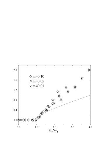
Figure 5: Rescaled baryon density vs. chemical potential together with the $\chi$PT predictions (5).

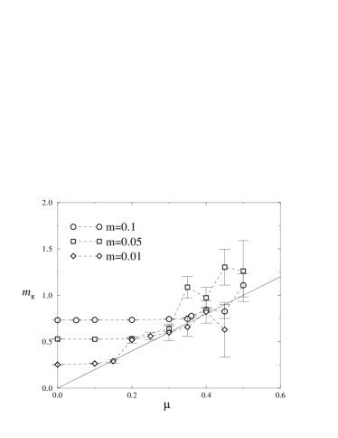
Figure 6: $m_{\pi}$ vs. $\mu$, for the three different quark masses. Also shown is the line $m_{\pi}=2\mu$.

In Hands:2000ei  we found indications that the onset transition at $x\approx 1$ may be delayed when the negative configurations are included using the TSMB algorithm. Here we have collected additional data with both algorithms from the region just above this transition point for $m=0.1$ (see table 2). The results are shown in figs. 7 and 8 for the chiral condensate and fermion density respectively. We can clearly see that the numbers for the positive determinant sector of TSMB agree well with the HMC data, giving the same early onset transition, but including the negative determinant sector brings the total average back so that it is consistent with the vacuum value — and inconsistent with the value in the positive determinant sector. We conclude from this that, as already indicated, the positive determinant sector and the full theory represent two different ‘physical’ models: the former describes a two-flavor theory with an onset transition at $\mu_{o}=m_{\pi}/2$, while the latter, the true $N=1$ theory, remains in the vacuum phase for $\mu>m_{\pi}/2$, and presumably has a transition to a normal or superconducting phase at higher $\mu$. At $\mu=0.4$ we see that the uncertainties in the averages of the full theory become large. This is an effect of the sign problem, which becomes serious at this point. Simulating at even larger chemical potential, in the hope of finding the real onset transition in this model, would be very demanding and beyond our current resources.

To gain further insight into the nature of the dense phase it is instructive to consider the quark energy density, given by

$$\epsilon_{\text{phys}}=\langle\bar{\chi}D_{0}\chi\rangle-{1\over 4}(3-m\langle\bar{\psi}\psi\rangle_{0})\,.$$ (7)

The results are shown in table 3, along with the expected energy density $nm_{\pi 0}/2$ of a system with quark number density $n$ consisting of non-interacting diquark baryons of mass $m_{\pi 0}$. The two sets of numbers are comparable, although to the accuracy we have obtained it is impossible to assess even the sign of the binding energy in such a picture. It is also possible to express things in physical units; since $m_{\pi}\propto\surd m$ Hands:2000ei , and observing that our value of $m/m_{\pi 0}\simeq 0.136$ is about 5 times the physical ratio (assuming $m_{u}=4$ MeV, $m_{\pi}=140$ MeV), we conclude that our $m=0.1$ simulation describes a world with $m\simeq 90$ MeV, $m_{\pi}\simeq 670$ MeV. This corresponds to a lattice spacing $a\simeq 0.22$ fm. At $\mu=0.37$ this gives a quark number density $n\simeq 3.6\text{ fm\,,}^{\!\!-3}$ with a corresponding energy density $\epsilon\simeq 1270\text{ MeV\,fm\,,}^{\!\!\!-3}$ considerably in excess of the nuclear matter values $n\simeq 0.48\text{ fm\,,}^{\!\!\!-3}$ $\epsilon\simeq 150\text{ MeV\,fm\,.}^{\!\!\!-3}$ Perhaps a more reasonable comparison, however, is the dimensionless ratio $\epsilon/(mn)$, which is $\simeq 3.8$ at $\mu=0.37$ but has a value closer to 80 in nuclear matter. This emphasises the large value of the quark mass in our simulations; a more “realistic” simulation would require a separate calibration, e.g. via the vector meson mass.

$\mu$	$\epsilon_{\text{phys}}$	${n\over 2}m_{\pi 0}$
0.20	0.0001(20)	0.0005(10)
0.30	$-0.0047(28)$	$-0.0007(12)$
0.35	$-0.0056(40)$	0.0020(18)
0.36	0.0042(31)	0.0074(15)
0.37	0.0148(51)	0.0142(24)
0.38	0.0188(80)	0.0226(40)
0.39	0.0316(70)	0.0302(30)
0.40	0.0609(83)	0.0536(37)
0.50	0.2688(220)	0.1921(88)

Table 3: Energy density as a function of $\mu$, compared with that of a system of non-interacting pions, for simulations with $m=0.1$.

Figure 7: The chiral condensate from TSMB and HMC simulations.

Figure 8: The fermion density from TSMB and HMC simulations.

In table 4 we report the susceptibility defined by the integrated pion correlator

$$\chi_{\pi}=\sum_{x}\langle\bar{\chi}\varepsilon\chi(0)\bar{\chi}\varepsilon\chi(x)\rangle=\sum_{x}G_{0,x}(\mu)G^{tr}_{0,x}(-\mu)\,,$$ (8)

where $\varepsilon(x)=(-1)^{x_{0}+x_{1}+x_{2}+x_{4}}$ and $G$ is the fermion propagator, which is real for adjoint quarks.

$\mu$	$\langle\chi_{\pi}\rangle_{\text{TSMB}}$	$\langle\chi_{\pi}\rangle_{+}$	$\langle\chi_{\pi}\rangle_{-}$	$\langle\chi_{\pi}\rangle_{\text{HMC}}$
0.00	45.87(7)
0.20				45.80(16)
0.30	45.76(5)			45.87(22)
0.35				45.36(25)
0.36	45.79(24)	45.28(21)	35.32(155)	45.04(17)
0.37	46.49(35)	44.80(22)	35.02(78)	44.18(21)
0.38	46.23(81)	42.49(30)	36.34(56)	42.91(45)
0.39				40.63(32)
0.40	46.24(321)	38.06(34)	35.56(38)	37.42(40)
0.50				21.15(82)

Table 4: Pion susceptibility $\chi_{\pi}$ from TSMB and HMC simulations.

In fact, the tabulated results come from ‘non-singlet’ diagrams with connected quark lines only; disconnected contributions were consistent with zero within large statistical uncertainties (we also attempted to measure the scalar susceptibility but did not find a significant signal with our statistics). The results are consistent, to within an irrelevant normalisation factor of 3, with the axial Ward identity $m\chi_{\pi}=\langle\bar{\psi}\psi\rangle$. Once again the HMC data and the positive determinant sector of TSMB are in close agreement, showing a systematic decrease of $\chi_{\pi}$ in the dense phase. Reweighting to the correct ensemble, however, again removes the evidence for the onset transition – this is significant since it demonstrates that reweighting also gives the expected behaviour for two-point correlation functions.

$\mu$	$m_{\pi}^{\text{TSMB}}$	$m_{\pi}^{+}$	$m_{\pi}^{-}$	$m_{\pi}^{\text{HMC}}$
0.00	0.7322(6)
0.20				0.7324(7)
0.30	0.7360(8)			0.7345(16)
0.35				0.7504(40)
0.36	2.00(85)	1.35(40)	—	0.7580(56)
0.37	0.686(81)	0.751(56)	2.06(30)	0.769(10)
0.38	1.29(65)	0.915(128)	—	0.758(22)
0.39				0.819(22)
0.40	1.19(2.52)	—	1.16(30)	0.829(28)

Table 5: The pion mass $m_{\pi}$ from TSMB and HMC simulations.

The pion mass $m_{\pi}(\mu)$ is extracted from the temporal decay of the correlator over timeslices 1–7. The results are shown in table 5. HMC results show that $m_{\pi}$ is constant and equal to $m_{\pi 0}$ for $\mu<\mu_{o}$, and increases for $\mu>\mu_{o}$ in approximate agreement with the $\chi$PT prediction (6); the fact that the results lie slightly above the $\chi$PT value is probably attributable to the small volume. It is interesting to contrast this behaviour with that observed in two-color QCD with fundamental staggered quarks Kogut:2001na , in which $m_{\pi}$ is observed to decrease once $\mu>\mu_{o}$. This behaviour is predicted by $\chi$PT Kogut:2000ek  for a pseudo-Goldstone meson with a flavor content symmetric under the residual global symmetry in the superfluid state, which for $N=2$ staggered adjoint flavors is Sp(2); $m_{\pi}$ should decrease with $\mu$ in a theory with Dyson index $\beta=4$ such as two-color QCD with staggered fundamental quarks, and increase if $\beta=1$ as is the case for the current model. It becomes very difficult to determine $m_{\pi}$ from the TSMB simulation once $\mu>0.3$, so we are not able to draw any significant conclusions from these data. However, the general tendency is compatible with what we observe for $\langle\bar{\psi}\psi\rangle$ and $n$; namely, that $m_{\pi}$ increases (with values compatible with those from HMC) when only positive determinant configurations are included, while it remains compatible with the $\mu=0$ value when all configurations are included.

3.3 Gauge field quantities

Our results for the plaquette and Wilson loops are given in table 6. Beyond the observation that both algorithms give consistent results for the plaquette we see no discernible effect over this range of chemical potentials — all quantities remain consistent with their values at $\mu=0$. At larger $\mu$ there is evidence that the plaquette starts to fall towards its quenched value due to the effects of Pauli blocking Hands:2000ei ; Hands:2000yh . The deviation of the $\mu=0.37$ values from the rest is probably a sign of insufficient statistics and/or a too short equilibration time.

$\mathcal{O}/\mu$	$\langle\mathcal{O}\rangle$	$\langle\mathcal{O}\rangle_{+}$	$\langle\mathcal{O}\rangle_{-}$	$\langle\mathcal{O}\rangle_{\text{HMC}}$
$\Box$
0.0	0.5667(9)
0.20				0.5667(16)
0.30	0.5689(12)			0.5677(20)
0.35				0.5689(20)
0.36	0.5687(20)	0.5684(19)	0.5623(27)	0.5644(30)
0.37	0.5584(15)	0.5583(14)	0.5572(21)	0.5642(35)
0.38	0.5696(15)	0.5688(12)	0.5676(13)	0.5677(35)
0.39				0.5685(30)
0.40	0.5579(38)	0.5597(18)	0.5602(19)	0.5676(40)
0.50				0.5634(50)
$\Box_{s}$
0.0	0.5667(9)
0.30	0.5688(13)
0.36	0.5686(19)	0.5683(19)	0.5625(30)
0.37	0.5595(15)	0.5590(15)	0.5566(22)
0.38	0.5687(18)	0.5682(14)	0.5667(15)
0.40	0.5583(43)	0.5600(20)	0.5602(21)
$W_{11}$
0.0	0.5668(9)
0.30	0.5687(12)
0.36	0.5691(22)	0.5688(22)	0.5617(26)
0.37	0.5574(14)	0.5575(14)	0.5579(21)
0.38	0.5696(15)	0.5688(13)	0.5676(16)
0.40	0.5575(41)	0.5593(17)	0.5599(18)
$W_{12}$
0.0	0.3426(14)
0.30	0.3452(16)
0.36	0.3463(33)	0.3459(32)	0.3375(37)
0.37	0.3291(19)	0.3292(19)	0.3294(29)
0.38	0.3474(22)	0.3462(20)	0.3443(21)
0.40	0.3299(59)	0.3320(25)	0.3326(28)
$W_{21}$
0.0	0.3422(14)
0.30	0.3451(18)
0.36	0.3458(35)	0.3543(34)	0.3356(36)
0.37	0.3289(22)	0.3292(21)	0.3308(28)
0.38	0.3451(26)	0.3453(21)	0.3457(23)
0.40	0.3296(60)	0.3321(25)	0.3328(28)
$W_{22}$
0.0	0.1408(15)
0.30	0.1439(18)
0.36	0.1460(35)	0.1456(35)	0.1377(39)
0.37	0.1268(22)	0.1269(21)	0.1279(28)
0.38	0.1478(30)	0.1477(24)	0.1474(25)
0.40	0.1303(68)	0.1318(31)	0.1323(33)
$L$
0.00	-0.003(3)
0.30	-0.005(4)
0.36	0.015(9)	0.014(9)	-0.002(10)
0.37	-0.002(4)	0.000(4)	0.011(7)
0.38	0.010(9)	0.008(7)	0.004(10)
0.40	-0.005(18)	-0.010(6)	-0.11(6)

Table 6: Results for the gauge observables: the plaquette $\Box$, spatial plaquette $\Box_{s}$, timelike Wilson loops $W_{ij}$, and Polyakov loop $L$.

The Polyakov loop $L$ on small lattices in the dense phase of two-color QCD with fundamental quarks was found to be small but non-zero in Kogut:2001na . Our results for the average Polyakov loop are also given in table 6. We can see that it remains zero everywhere, and conclude that there is no sign of any deconfinement transition either in the positive determinant sector or in the full theory.

3.4 Diquark condensation

A natural explanation of the agreement between the HMC and positive determinant results and $\chi$PT predictions is that the positive determinant sector mimics a theory with two flavors: one quark and one ‘conjugate quark’ Stephanov:1996ki . We may cast further light on this by studying the behaviour of the diquark condensate (1) expected in the two-flavor theory. This condensate may be determined by introducing a diquark source term in the action, which now describes two flavors,

$$S[j]=S+j\sum_{x}qq_{\bf 3}(x)\,,$$ (9)

extracting the condensate $\langle qq_{\bf 3}(j)\rangle\!=\!V^{-1}\partial\ln Z[j]/\partial j$, and extrapolating the results to $j=0$ Morrison:1998ud . Here, we have only performed ‘partially quenched’ measurements — i.e., we have included a nonzero diquark source $j$ in the measurement of observables from configurations generated at $j=0$.

In figure 9 we show the chiral and two-flavor diquark condensates from our HMC simulations as a function of $j$ for a number of values of the chemical potential. Note that on a finite system at $j=0$ the diquark condensate is identically zero. We have therefore excluded this point from our plot.

Figure 9: The chiral and diquark condensates as a function of the chemical potential $\mu$ and the diquark source $j$, from HMC.

The extrapolation $j\to 0$ needs some discussion. To leading order in $\chi$PT the relation between chiral and diquark condensates, $m$, and $j$ is Kogut:2000ek

$$x^{2}\langle\bar{\psi}\psi\rangle\langle qq_{\bf 3}\rangle=\frac{\langle\bar{\psi}\psi\rangle_{0}}{\sqrt{1+\frac{j^{2}}{m^{2}}}}\left[\langle qq_{\bf 3}\rangle-\frac{j}{m}\langle\bar{\psi}\psi\rangle\right],$$ (10)

together with the constraint

$$\langle\bar{\psi}\psi\rangle_{0}^{2}=\langle\bar{\psi}\psi\rangle^{2}+\langle qq_{\bf 3}\rangle^{2}.$$ (11)

If we assume $j\ll m$ and ignore quadratic terms, then at at the critical point $x_{o}=1$ the resulting cubic equation yields $\langle qq_{\bf 3}\rangle/\langle\bar{\psi}\psi\rangle_{0}=^{3}\!\!\!\!\!\surd 2({j\over m})^{1\over 3}-{2\over 3}{j\over m}$. We have therefore tried to fit the data using the form

$$\langle qq_{\bf 3}(j)\rangle=A+Bj^{1\over 3}+Cj\,.$$ (12)

The results of the extrapolation are shown in fig. 10. Positive values for the coefficient $A$ were found for $\mu\geq 0.36$, and the quality of the fit improved as $\mu$ increased. At $\mu=0.36$ the values for the coefficients were $A=0.062(15)$, $B=9.37(7)$, $C=-16.1(2)$, the latter to be compared with $\chi$PT predictions at $x_{o}=1$ of 8.28 and -20.4 respectively. Although the quality of the fits improves as $\mu$ increases, the curvature due to the $j^{1\over 3}$ term is observed to manifest itself principally at values of $j<0.01$, i.e., below where we have data. We therefore suspect that fits to (12) underestimate $\langle qq_{\bf 3}(j=0)\rangle$ for $\mu>\mu_{o}$. This is in line with the solutions of (10,11) at $x>1$: extrapolating the solutions of (10) at $j>0$ to $j=0$ using (12) always yields a lower value than the actual solution at $j=0$,

$$\langle qq_{\bf 3}\rangle=\langle\bar{\psi}\psi\rangle_{0}\sqrt{1-\frac{1}{x^{4}}}\,.$$ (13)

We can also see from fig. 9 that the behaviours of $\langle\bar{\psi}\psi\rangle$ and $\langle qq_{\bf 3}\rangle$ are strongly anti-correlated. This is a result of the two quantities being connected by a $\operatorname{U}(4)_{f}$ transformation Hands:2000ei ,

$$X=\begin{pmatrix}\chi_{o}\\ \bar{\chi}_{o}^{tr}\end{pmatrix}\to VX\quad\bar{X}=\begin{pmatrix}\bar{\chi}_{e}&\chi_{e}^{tr}\end{pmatrix}\to\bar{X}V^{\dagger}\,,$$ (14)

with

$$V=\frac{1}{2}\begin{pmatrix}\phantom{i}P&iP^{tr}\\ iP&\phantom{i}P^{tr}\\ \end{pmatrix}\quad\text{where}\quad P=\begin{pmatrix}1&-1\\ 1&\phantom{-}1\\ \end{pmatrix}.$$ (15)

The superfluid transition in this model is expected to be realised by the chiral condensate ‘rotating’ into the diquark condensate, in such a way that the constraint (11) is maintained. This has been shown to be the case to leading order in $\chi$PT Kogut:2000ek . At next to leading order, however, some dependence on $\mu$ and $j$ is expected Splittorff:2001fy .

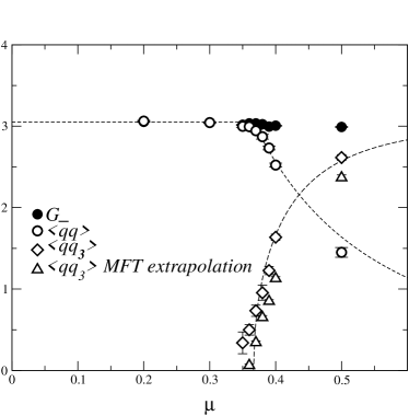
Figure 10: $\langle\bar{\psi}\psi\rangle$, $\langle qq_{\bf 3}\rangle$ and $G$ versus $\mu$, together with predictions from leading order $\chi$PT. “MFT extrapolation” denotes points from fits to (12)

We have therefore tried a second method in which the quantity $G^{2}=\langle\bar{\psi}\psi\rangle^{2}+\langle qq_{\bf 3}\rangle^{2}$ measured for $j>0$ is extrapolated to $j=0$ using a second order polynomial. Fig. 11 shows that $G^{(}j,\mu)$ exhibits relatively little variation with either $j$ or $\mu$, implying that the NLO $\chi$PT corrections are small. Note that since $\langle qq_{\bf 3}(j=0)\rangle\equiv 0$, the extrapolated $G^{(}0)$ lies considerably above the numerical data for $\mu>\mu_{o}$. We now use $G^{(}0)$, which appears to vary very little across the transition at $\mu=\mu_{o}$, together with $\langle\bar{\psi}\psi\rangle$ to extract $\langle qq_{\bf 3}\rangle$; the results are plotted in fig. 10. In this case difficulties associated with taking the difference of two fluctuating quantities means that the method is probably not accurate for $\langle qq_{\bf 3}\rangle$ in the immediate vicinity of the critical point; for $\mu\geq 0.37$, however, the agreement with the $\chi$PT predictions (4,13) is striking.

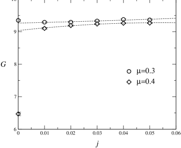
Figure 11: The quantity $G^{2}(j)$ for values of $\mu$ in either phase. Lines show the quadratic extrapolation to $j=0$.

In figure 12 we compare the HMC results for $\langle qq_{\bf 3}\rangle$ at $\mu=0.38$ with TSMB numbers. Since the superfluid transition is not present for $N=1$, the diquark condensate should be suppressed, and indeed the data from the full theory lie lower and exhibit a stronger negative curvature than the positive determinant data. It is, however, not possible to conclude from these data whether the one set will extrapolate to zero and the other to a non-zero value, especially taking into account the problems discussed above.

Figure 12: The diquark condensate as a function of the diquark source $j$ at $\mu=0.38$, from TSMB and HMC.

Figure 13: The superconducting (top) and superfluid (bottom) diquark susceptibilites as a function of the chemical potential $\mu$, from HMC and TSMB.

We have also computed the following four-point functions, which we refer to as superfluid and superconducting “susceptibilities”:

$$\chi_{\bf 3} =\langle\bar{\chi}(x)\varepsilon\bar{\chi}^{tr}(x)\chi^{tr}(x)\varepsilon\chi(x)\rangle\,,$$ (16)

$$\chi_{sc} =\frac{1}{3}\langle\bar{\chi}(x)t^{i}\bar{\chi}^{tr}(x)\chi^{tr}(x)t^{i}\chi(x)\rangle\,.$$ (17)

Both may be computed without introducing a diquark source term in the action Hands:1998kk ; Morrison:1998ud , and are related to the superfluid and superconducting diquark condensates of eqs. (1) and (2) respectively. Both are scalar objects corresponding to the local component of a diquark susceptibility $\chi_{qq}=\sum_{x}\langle qq(0)\bar{q}\bar{q}(x)\rangle$ which we might expect to increase significantly if condensation occurs. Note, however, that $\chi_{sc}$ in (17) is the only such contribution which is gauge invariant and hence a possible signal of color superconductivity in a simulation (to be compared with $\Phi^{\dagger}\Phi$ in a Higgs model). To be able to compare signals for condensation between channels we have therefore chosen the local operators (16,17) over the full susceptibilities.

Figure 13 shows the superfluid and superconducting diquark susceptibilities as a function of chemical potential from our HMC and TSMB simulations. In the low density regime $\chi_{\bf 3}$ and $\chi_{sc}$ show little variation with $\mu$ and are roughly equal. Once we enter the superfluid phase for $\mu>\mu_{o}$, however, signals for both observables become increasingly dominated by very sharp peaks of amplitude $O(10-20)$, the distinction being that for $\chi_{\bf 3}$ the peaks are all positive whereas for $\chi_{sc}$ they occur with either sign. Such peaks are characteristic of localised small-eigenvalue modes of $D{\!\!\!\!/\,}$, of which there are many in the dense phase Hands:2000ei . For $\mu>\mu_{o}$, in the positive determinant sector $\chi_{sc}$ decreases. We interpret this as an effect of Pauli blocking or phase space suppression: as the ground state is filled up by fermions, there is less phase space left to accommodate the fermion loops that contribute to $\chi_{sc}$.

When the sign is taken into account, this effect, like other effects of the superfluid transition, disappears. Perhaps surprisingly, this is in fact the cleanest signal we have of the effect of the sign of the determinant on observables. By way of contrast, $\chi_{\bf 3}$ shows a small increase as the onset transition is reached, as one would expect as a result of a Goldstone mode once a superfluid condensate forms. However, there is a large deviation between $\chi_{\bf 3}$ as measured in HMC and TSMB(+); this is the only observable we have examined in which the two algorithms significantly fail to agree. One possible explanation is that Goldstone physics is extremely sensitive to small eigenmodes of $D{\!\!\!\!/\,}$. In HMC such modes are responsible for large force terms and reduced acceptance rates; moreover the sampling may not be correct due to the breakdown of ergodicity Hands:2000ei . Hybrid algorithms have produced disparate results for susceptibilities in the dense phase Morrison:1998ud ; Hands:1999md . TSMB, in contrast, tends to over-sample configurations with small modes, correcting this by reweighting factors with modulus less than 1. In fact, in this case some of the eigenvalues and reweighting factors are very small, and therefore problems with numerical accuracy cannot be excluded. It is perhaps not surprising that the algorithms disagree in this exacting regime. We were not able to obtain any result for the overall superfluid susceptibility in TSMB (i.e., with the negative determinant sector included) due to huge fluctuations in the signal.

4 Conclusions

We have studied two-color QCD with one flavor of staggered quark in the adjoint representation. We have employed two different simulation algorithms, and have continued to gain insight into the optimal tuning of the TSMB algorithm in the high density regime. This is the preferred algorithm not only because as highlighted in Hands:2000ei  it is capable of maintaining ergodicity via its ability to change the determinant sign once $\mu>\mu_{o}$, but also because it more effectively samples small eigenmodes, which are important in the presence of a physical Goldstone excitation. We find that the positive determinant sector behaves like a two-flavor model, and exhibits good agreement with chiral perturbation theory predictions for such a model in the regime $1<x<2$. At higher chemical potentials there are preliminary indications of a breakdown of $\chi$PT, and possible signs of a further phase transition. However, data from larger volumes and smaller bare quark masses would be needed to make these observations definitive.

Above the onset transition in the positive determinant sector, we have successfully obtained a signal for a non-zero two-flavor diquark condensate $\langle qq_{\bf 3}\rangle$, indicating a superfluid ground state for $\mu>m_{\pi}/2$. The chiral condensate rotates into this diquark condensate, in good quantitative agreement with the behaviour predicted by $\chi$PT. This feature also enabled us to achieve reasonable control over the necessary $j\to 0$ extrapolation. We also find that the superfluid susceptibility (16) increases, while the superconducting susceptibility (17) decreases for $\mu>\mu_{o}$. For the former there are indications of a lack of consistency between HMC and TSMB algorithms, indicative of the two methods’ differing treatment of small eigenmodes. The latter may be interpreted as an effect of phase space suppression. Unfortunately we have seen no evidence for a superconducting condensate $\langle qq^{i}_{sc}\rangle\not=0$, one of our original motivations for studying the model.

When the negative determinant configurations are included in the measurement, the onset transition and diquark condensation disappear. This is what we would expect for the one-flavor model and is consistent with the Exclusion Principle. There is much stronger evidence for this scenario than that presented in our previous paper Hands:2000ei , providing a conclusive demonstration, should any still be needed, that the determinant sign plays a decisive role in determining the ground state of systems with $\mu\not=0$. Unfortunately, the severity of the sign problem means we have not been able to locate the real onset transition for this model.

- (1) K. Rajagopal and F. Wilczek, The condensed matter physics of QCD, in At the Frontier of Particle Physics: Handbook of QCD, edited by M. Shifman, p. 2061, Singapore, 2001, World Scientific, hep-ph/0011333.
- (2) M. Alford, hep-ph/0102047.
- (3) D. Bailin and A. Love, Phys. Rept. 107, 325 (1984).
- (4) M. Alford, K. Rajagopal, and F. Wilczek, Phys. Lett. B422, 247 (1998), hep-ph/9711395.
- (5) R. Rapp, T. Schäfer, E. Shuryak, and M. Velkovsky, Phys. Rev. Lett. 81, 53 (1998), hep-ph/9711396.
- (6) M. Alford, K. Rajagopal, and F. Wilczek, Nucl. Phys. B537, 443 (1999), hep-ph/9804403.
- (7) D. Son and M. Stephanov, Phys. Rev. Lett. 86, 592 (2001), hep-ph/0005225.
- (8) S. Hands and S. E. Morrison, Phys. Rev. D59, 116002 (1999), hep-lat/9807033.
- (9) S. Hands, B. Lucini, and S. Morrison, Phys. Rev. Lett. 86, 753 (2001), hep-lat/0008027; hep-lat/0109001.
- (10) J. Kogut, M. Stephanov, and D. Toublan, Phys. Lett. B464, 183 (1999), hep-ph/9906346.
- (11) J. Kogut, M. Stephanov, D. Toublan, J. Verbaarschot, and A. Zhitnitsky, Nucl. Phys. B582, 477 (2000), hep-ph/0001171.
- (12) K. Splittorff, D. Son, and M. Stephanov, Phys. Rev. D64, 016003 (2001), hep-ph/0012274.
- (13) A. Nakamura, Phys. Lett. B149, 391 (1984).
- (14) E. Dagotto, A. Moreo, and U. Wolff, Phys. Lett. B186, 395 (1987).
- (15) J. Klatke and K. Mütter, Nucl. Phys. B342, 764 (1990).
- (16) S. Morrison and S. Hands, Two colours QCD at nonzero chemical potential, in Strong and Electroweak Matter, Copenhagen, 1998, p. 364, 1999, hep-lat/9902012.
- (17) S. Hands, J. B. Kogut, M.-P. Lombardo, and S. E. Morrison, Nucl. Phys. B558, 327 (1999), hep-lat/9902034.
- (18) R. Aloisio, V. Azcoiti, G. Di Carlo, A. Galante, and A. F. Grillo, Phys. Lett. B493, 189 (2000), hep-lat/0009034; Nucl. Phys. B606, 322 (2001), hep-lat/0011079.
- (19) E. Bittner, M.-P. Lombardo, H. Markum, and R. Pullirsch, Nucl. Phys. Proc. Suppl. 94, 445 (2001), hep-lat/0010018.
- (20) Y. Liu, O. Miyamura, A. Nakamura, and T. Takaishi, hep-lat/0009009.
- (21) S. Muroya, A. Nakamura, and C. Nonaka, Nucl. Phys. Proc. Suppl. 94, 469 (2001), hep-lat/0010073.
- (22) J. Kogut, D. Sinclair, S. Hands, and S. Morrison, hep-lat/0105026.
- (23) J. B. Kogut, D. Toublan, and D. Sinclair, Phys. Lett. B514, 77 (2001), hep-lat/0104010.
- (24) S. Hands et al., Eur. Phys. J. C17, 285 (2000), hep-lat/0006018.
- (25) S. Hands, I. Montvay, M. Oevers, L. Scorzato, and J. Skullerud, Nucl. Phys. Proc. Suppl. 94, 461 (2001), hep-lat/0010085.
- (26) M. Stephanov, Phys. Rev. Lett. 76, 4472 (1996), hep-lat/9604003.
- (27) I. Montvay, Nucl. Phys. B466, 259 (1996), hep-lat/9510042.
- (28) I. Montvay, Multi-bosonic algorithms for dynamical fermion simulations, in Molecular dynamics on parallel computers, World Scientific, 2000, hep-lat/9903029.
- (29) K. Splittorff, D. Toublan, and J. Verbaarschot, hep-ph/0108040.