Spectral function at high temperature HD-THEP-01-39

Abstract

For a weakly coupled quantum field at high temperature the classical approximation offers a possibility to gain insight into nonperturbative real-time dynamics. I use this to present a nonperturbative approach to the computation of spectral functions in real time. Results are shown for a scalar field in $2+1$ dimensions.

1. In thermal equilibrium spectral functions contain all available information since other real- (and imaginary-) time correlators are related to them via the KMS condition. A nonperturbative computation of spectral functions seems therefore desirable; nonperturbative in order to:

• deal with a truly nonperturbative theory, such as the infrared sector of high-temperature nonabelian gauge fields,

• investigate the utility of (resummed) perturbative ideas, since weak coupling $+$ high temperature $\neq$ simple.

For the calculation of static quantities, such as free energies, phase diagrams and screening masses, the euclidean lattice formulation of finite-temperature quantum fields offers a first-principle approach. For intrinsically real-time correlators, such as the spectral function, no first-principle nonperturbative formulation exists. In the last ${\cal O}(10)$ years the classical approximation at high temperature and weak coupling has provided much insight into real-time dynamics, see [1, 2] for recent reviews. In this talk I discuss how spectral functions can be computed in the classical approximation and what can be learned from them. Details can be found in [3].

2. The spectral function for a bosonic operator $O$ can be defined as the thermal expectation value

$$\rho(x-y)=i\langle[O(x),O^{\dagger}(y)]_{-}\rangle.$$ (1)

Other two-point functions can be expressed in terms of it using the KMS condition, leading to the appearance of the Bose distribution function $n(\omega)=1/[e^{\omega/T}-1]$. For example, the euclidean correlator $D(\tau,{\mathbf{x}})=\langle O(\tau,{\mathbf{x}})O^{\dagger}(0,{\mathbf{0}})\rangle_{E}$, with imaginary time $\tau\in[0,1/T]$, is related to the spectral function via the integral equation

$$D(\tau,{\mathbf{p}})=\int_{0}^{\infty}\frac{{\rm d}\omega}{2\pi i}\,K(\tau,\omega)\rho(\omega,{\mathbf{p}}),$$ (2)

with the kernel

$$K(\tau,\omega)=n(\omega)\left[e^{\omega\tau}+e^{-\omega(\tau-1/T)}\right]$$ (3)

obeying $K(\tau,\omega)=-K(\tau,-\omega)=K(1/T-\tau,\omega)$. The extraction of the spectral function from the euclidean lattice correlator is a highly nontrivial inversion problem, currently tackled using the Maximal Entropy Method [4]. In real time the spectral function would be accessible directly without the need to solve an integral equation.

The classical approximation provides a nonperturbative computational scheme in real time. In the classical limit $-i$ times the commutator is replaced with the Poisson bracket and the classical spectral function reads

$$\rho_{\rm cl}(x-y)=-\langle\{O(x),O^{\dagger}(y)\}\rangle_{\rm cl}.$$ (4)

The time evolution is determined by the classical equations of motion, evolving from some initial condition. The brackets $\langle\cdot\rangle_{\rm cl}$ denote a Boltzmann-weighted average over these initial conditions.

In perturbation theory the relation between classical and quantum physics at finite temperature can be seen clearly. Consider a self-interacting scalar field with coupling constant $\lambda$. The effective expansion parameter is $\hbar\lambda n(\hbar\omega)$ (with the $\hbar$ dependence indicated explicitly). As a result, in the classical limit each loop contributes with a proportionality factor $\lambda T/\omega$. Note that this implies that the infrared sector ($\hbar\omega/T\ll 1$) is essentially classical but that in the ultraviolet problems are encountered (the Rayleigh-Jeans divergence, see below).

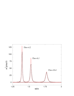
Figure 1: Spectral functions $\rho_{\rm cl}(\omega,{\mathbf{0}})$ for various temperatures $T$. Fits to a Breit-Wigner function are shown with dotted lines.

For actual calculations, the Poisson bracket in Eq. (4) appears difficult to use numerically, but in equilibrium the KMS condition comes to the rescue. In the classical limit the KMS relation relates the statistical correlator $S(x-y)=\langle O(x)O^{\dagger}(y)\rangle_{\rm cl}$ and the spectral function in momentum space as

$$-i\frac{T}{\omega}\rho_{\rm cl}(\omega,{\mathbf{p}})=S(\omega,{\mathbf{p}}).$$ (5)

or equivalently in real-space as

$$\rho_{\rm cl}(t,{\mathbf{x}})=-\frac{1}{T}\partial_{t}S(t,{\mathbf{x}}).$$ (6)

The latter relation, valid for arbitrary $O$, allows an easy calculation of classical spectral functions.

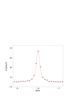
Figure 2: As in Fig. 1 at $T/m=7.2$. The actual data points are presented with squares.

3. To illustrate the method we consider a simple real scalar field with a $\lambda\phi^{4}$/4!-interaction in the symmetric phase in $2+1$ dimensions (note that in a classical theory the dimensionless coupling $\lambda/m$ can be taken equal to 1 without loss of generality). We focus on the one-particle spectral function. According to the classical KMS condition we have to compute

$$\rho_{\rm cl}(t,{\mathbf{x}})\!\!\!\! = \!\!\!\!-\langle\{\phi(t,{\mathbf{x}}),\phi(0,{\mathbf{0}})\}\rangle_{\rm cl}$$ (7)

$$= \!\!\!\!-\frac{1}{T}\langle\pi(t,{\mathbf{x}})\phi(0,{\mathbf{0}})\rangle_{\rm cl},$$

where $\pi=\partial_{t}\phi$ is the canonical momentum. The right-hand-side is a simple correlation function that can be computed numerically without any problems [3]. The theory is defined on a spatial lattice of $N\times N$ sites and lattice spacing $a$ (we used $N=128,ma=0.2$, and periodic boundary conditions). The classical equations of motion are solved with a leapfrog algorithm with time step $a_{0}/a=0.1$. Thermal initial configurations are generated with the Kramers equation algorithm (the plots shown are obtained with 2000 independently thermalized initial configurations). On the lattice the spectral function (7) is symmetrized:

$$\rho_{{\rm cl},\rm lat}(t,{\mathbf{x}})\!\!\!\! =$$ (8)

$$\!\!\!\!\!\!\!\!\!\!\!\!\!\!\!\!\!\!\!\!\!\!\!\!\!\!\!\!\!\!\!\!\!\!-\frac{1}{T}\left\langle\pi(t+\frac{1}{2}a_{0},{\mathbf{x}})\frac{1}{2}\left[\phi(0,{\mathbf{0}})+\phi(a_{0},{\mathbf{0}})\right]\right\rangle_{\rm cl}\!.$$

The simulations give the spectral function as a correlation function in real time. A sine transform (using symmetry properties of the spectral function under time reflection and complex conjugation) yields the desired result as a function of frequency. In Fig. 1 the spectral function at zero momentum is shown for various temperatures and in Fig. 2 a magnification with the actual data points indicated is presented. The maximal (real) time $t_{\rm max}$ used in the analysis constrains the resolution in frequency space to $\Delta\omega=\pi/t_{\rm max}$, but this poses no problem ($\Delta\omega/m\approx 0.01$ in Fig. 2).

Figure 3: Temperature dependence of the mass $M$ (circles) and width $\Gamma$ (squares, multiplied by 25 for clarity), obtained from fits to a Breit-Wigner function. Errors are determined with a jackknife analysis. The resummed perturbative predictions are shown with lines.

4. It is now clear that spectral functions can be computed nonperturbatively in classical thermal field theory. The question is what we may learn for hot quantum fields.

As alluded to above, the setup of perturbation theory in the quantum and classical case is similar and the results may be used to address the applicability of (resummed) perturbation theory. In the weak-coupling regime the spectral function is dominated by the plasmon. A simple way to parametrize it (ignoring the proper analytical structure) is by a Breit-Wigner spectral function. At zero momentum it reads

$$\rho_{\rm BW}(\omega)=\frac{2\omega\Gamma}{(\omega^{2}-M^{2})^{2}+\omega^{2}\Gamma^{2}}.$$ (9)

Fits of the data to a Breit-Wigner function are shown in Figs. 1,2, and yield nonperturbatively determined values of the plasmon mass and width. These can be compared with the perturbative predictions. At lowest order the mass parameter $M$ is determined from the classical limit of the standard one-loop gap equation. The leading contribution to the width $\Gamma$ comes from the two-loop setting-sun diagram and on dimensional grounds it is $\Gamma=c\lambda^{2}T^{2}/M^{3}$, with a small coefficient $c=(3-2\sqrt{2})/(32\pi)$ [3]. A comparison between the perturbatively and nonperturbatively determined values of the effective mass and width is shown in Fig. 3. A nice agreement can be seen, indicating that for this range of parameters perturbation theory is reliable.

5. It is straightforward to extend the calculation to more complicated spectral functions in scalar and gauge theories (for lattice fermions in real time, see [5]). Transport coefficients can be defined from the zero-momentum and zero-frequency limit of equilibrium spectral functions of appropriate composite operators. Simple power counting shows that these quantities are dominated by hard ($\sim T$) momenta. In a classical calculation they will therefore be sensitive to the lattice regulator. In fact, such dependence has already been encountered since the effective mass parameter $M$ depends (logarithmically in $2+1$ dimensions) on the lattice cutoff. However, as can be seen from Fig. 3, this does not automatically imply that the classical findings cannot be used: analytical perturbative and numerical nonperturbative calculations can still be compared, provided the role of the lattice regulator is incorporated properly.

Acknowledgements: I thank Nucu Stamatescu for discussions. Supported by the TMR network, EU contract no. FMRX-CT97-0122.

References

- [1] D. Bödeker, Nucl. Phys. Proc. Suppl. 94 (2001) 61 [hep-lat/0011077].
- [2] L. G. Yaffe, these Proceedings.
- [3] G. Aarts, Phys. Lett. B 518 (2001) 315 [hep-ph/0108125].
- [4] I. Wetzorke and F. Karsch, hep-lat/0008008, and various contributions to these Procs.
- [5] G. Aarts and J. Smit, Nucl. Phys. B 555 (1999) 355 [hep-ph/9812413].