Calculating the $I=2$ Pion Scattering Length Using Tadpole Improved Clover Wilson Action on Coarse Anisotropic Lattices

Abstract

In an exploratory study, using the tadpole improved clover Wilson quark action on small, coarse and anisotropic lattices, the $\pi\pi$ scattering length in the $I=2$ channel is calculated within quenched approximation. A new method is proposed which enables us to make chiral extrapolation of our lattice results without calculating the decay constant on the lattice. Finite volume and finite lattice spacing errors are analyzed and the results are extrapolated towards the infinite volume and continuum limit. Comparisons of our lattice results with the new experiment and the results from Chiral Perturbation Theory are made. Good agreements are found.

1 Introduction

It has become clear that anisotropic, coarse lattices and improved lattice actions are ideal candidates for lattice QCD calculations on small computers [1, 2, 3, 4]. They are particularly advantageous for heavy objects like the glueballs, one meson states with nonzero spatial momenta and multi-meson states with or without spatial momenta. The gauge action employed is the tadpole improved gluonic action on anisotropic lattices:

$$S= - \beta\sum_{i>j}\left[{5\over 9}{TrP_{ij}\over\xi u^{4}_{s}}-{1\over 36}{TrR_{ij}\over\xi u^{6}_{s}}-{1\over 36}{TrR_{ji}\over\xi u^{6}_{s}}\right]$$ (1)

$$- \beta\sum_{i}\left[{4\over 9}{\xi TrP_{0i}\over u^{2}_{s}}-{1\over 36}{\xi TrR_{i0}\over u^{4}_{s}}\right]\;\;,$$

where $P_{0i}$ and $P_{ij}$ represents the usual temporal and spatial plaquette variable, respectively. $R_{ij}$ and $R_{i0}$ designates the $2\times 1$ spatial and temporal Wilson loops, where, in order to eliminate the spurious states, we have restricted the coupling of fields in the temporal direction to be within one lattice spacing. The parameter $u_{s}$, which is taken to be the fourth root of the average spatial plaquette value, is the tadpole improvement parameter determined self-consistently from the simulation. With this tadpole improvement factor, the renormalization of the anisotropy (or aspect ratio) $\xi=a_{s}/a_{t}$ will be small. Therefore, we will not differentiate the bare aspect ratio and the renormalized one in this work. Using this action, glueball and hadron spectra have been studied within quenched approximation [3, 4, 5, 6, 7, 8, 9]. In this paper, we would like to present our results on the pion-pion scattering lengths within quenched approximation. Main results of this paper has already been reported in [10]. Some details of the calculation are presented in this paper.

Lattice calculations of pion scattering lengths have been performed by various authors using symmetric lattices without the improvement [11, 12, 13]. It turned out that, using the symmetric lattices and Wilson action, large lattices have to be simulated which require substantial amount of computing resources. It becomes even more challenging if the chiral, infinite volume and continuum limits are to be studied [13]. In this exploratory study, we would like to show that, such a calculation is feasible using relatively small lattices, typically of the size $8^{3}40$, with the tadpole improved anisotropic lattice actions. Attempts are also made to study the chiral, infinite volume and continuum limits extrapolation in a more systematic fashion. The final extrapolated result on the pion-pion scattering length in the $I=2$ channel is compared with the new experimental result from E865 collaboration [14] and Chiral Perturbation Theory [15, 16, 17, 18] with encouraging results. Of course, more accurate lattice calculations of the pion scattering length will inevitably require lattices larger than the ones studied in this paper.

The fermion action used in this calculation is the tadpole improved clover Wilson action on anisotropic lattices [19, 20]:

$${\mathcal{M}}_{xy} = \delta_{xy}\sigma+{\mathcal{A}}_{xy}$$

$${\mathcal{A}}_{xy} = \delta_{xy}\left[{1\over 2\kappa_{\max}}+\rho_{t}\sum^{3}_{i=1}\sigma_{0i}{\mathcal{F}}_{0i}+\rho_{s}(\sigma_{12}{\mathcal{F}}_{12}+\sigma_{23}{\mathcal{F}}_{23}+\sigma_{31}{\mathcal{F}}_{31})\right]$$ (2)

$$- \sum_{\mu}\eta_{\mu}\left[(1-\gamma_{\mu})U_{\mu}(x)\delta_{x+\mu,y}+(1+\gamma_{\mu})U^{\dagger}_{\mu}(x-\mu)\delta_{x-\mu,y}\right]\;\;,$$

where various coefficients in the fermion matrix ${\mathcal{M}}$ are given by:

$$\eta_{i} = \nu/(2u_{s})\;\;,\;\;\eta_{0}=\xi/2\;\;,\;\;\sigma=1/(2\kappa)-1/(1\kappa_{max})\;\;,$$

$$\rho_{t} = c_{SW}(1+\xi)/(4u^{2}_{s})\;\;,\;\;\rho_{s}=c_{SW}/(2u^{4}_{s})\;\;.$$ (3)

Among the parameters which appear in the fermion matrix, $c_{SW}$ is the coefficient of the clover term and $\nu$ is the so-called bare velocity of light, which has to be tuned non-perturbatively using the single pion dispersion relations [20]. Tuning the clover coefficients non-perturbatively is a difficult procedure. In this work, only the tadpole improved tree-level value is used instead.

In the fermion matrix (1), the bare quark mass dependence is singled out into the parameter $\sigma$ and the matrix ${\mathcal{A}}$ remains unchanged if the bare quark mass is varied. Therefore, the shifted structure of the matrix ${\mathcal{M}}$ can be utilized to solve for quark propagators at various values of valance quark mass $m_{0}$ (or equivalently $\kappa$) at the cost of solving only the lightest valance quark mass value at $\kappa=\kappa_{\max}$, using the so-called Multi-mass Minimal Residual ($M^{3}R$ for short) algorithm [21, 22, 23]. This is particularly advantageous in a quenched calculation since one needs the results at various quark mass values to perform the chiral extrapolation.

This paper is organized in the following manner. In Section 2, the method to calculate $\pi\pi$ scattering length is reviewed. In Section 3, some simulation details are described. In Section 4, our results of the scattering lengths obtained on lattices of various sizes and lattice spacings are extrapolated towards the chiral limit. A new quantity is proposed which is easier to measure on the lattice and has a simpler chiral behavior than the scattering length itself. Finite size effects are studied and two schemes of extrapolating to the infinite volume limit are studied. Finally, our lattice results are extrapolated towards the continuum limit. Comparisons with the experimental value and values from chiral perturbation theory at various orders are also discussed. In Section 5, we conclude with some general remarks.

2 Formulation to extract the scattering length

In order to calculate hadron scattering lengths on the lattice, or the scattering phase shifts in general, one uses Lüscher’s formula which relates the exact energy level of two hadron states in a finite box to the scattering phase shift in the continuum. In the case of two pions which scatter at zero relative three momentum, this formula then relates the exact two pion energy $E^{(I)}_{\pi\pi}$ in a finite box of size $L$ and isospin $I$ channel to the corresponding scattering length $a^{(I)}_{0}$ in the continuum. This formula reads [24]:

$$E^{(I)}_{\pi\pi}-2m_{\pi}=-\frac{4\pi a^{(I)}_{0}}{m_{\pi}L^{3}}\left[1+c_{1}\frac{a^{(I)}_{0}}{L}+c_{2}(\frac{a^{(I)}_{0}}{L})^{2}\right]+O(L^{-6})\;\;,$$ (4)

where $c_{1}=-2.837297$, $c_{2}=6.375183$ are numerical constants. In this paper, this formula will be utilized to calculate the pion-pion scattering length $a^{(2)}_{0}$ in the $I=2$ channel, which then requires the determination of the corresponding energy shift $\delta E^{(2)}_{\pi\pi}\equiv E^{(2)}_{\pi\pi}-2m_{\pi}$ in that channel.

One issue that one has to keep in mind is that, in a quenched calculation, Lüscher’s formula (4) has to be modified dramatically as discussed in [25]. Due to the anomalous contributions in quenched chiral perturbation theory from $\eta^{\prime}$, the energy shifts are contaminated by terms that might be of order $L^{0}=1$ and $L^{-2}$ in the $I=0$ channel. If these contributions were substantial, extraction of the corresponding scattering length from the energy shift might become problematic. In the $I=2$ channel, the situation is better. The quenched chiral corrections modify the energy shift by terms that are at least of order $L^{-3}$ with usually small coefficients. Therefore, doing quenched calculation in the $I=2$ channel is safer.

To measure the pion mass $m_{\pi}$ and to extract the energy shift $\delta E^{(2)}_{\pi\pi}$ of two pions with zero relative momentum, we construct the correlation functions from the corresponding operators in the $I=2$ channel. We have used the operators proposed in Ref. [12]. First, the local operators which create a single pion with appropriate isospin values are:

$$\pi^{+}({\bf x},t) = -\bar{d}({\bf x},t)\gamma_{5}u({\bf x},t)\;\;,\;\;\pi^{-}({\bf x},t)=\bar{u}({\bf x},t)\gamma_{5}d({\bf x},t)\;\;,\;\;$$

$$\pi^{0}({\bf x},t) = {1\over\sqrt{2}}[\bar{u}({\bf x},t)\gamma_{5}u({\bf x},t)-\bar{d}({\bf x},t)\gamma_{5}d({\bf x},t)]\;\;,$$ (5)

where $u({\bf x},t)$, $d({\bf x},t)$, $\bar{u}({\bf x},t)$ and $\bar{d}({\bf x},t)$ are basic local quark fields corresponding to $u$ and $d$ quarks respectively. The operators which correspond to zero momentum single pions are:

$$\pi^{a}_{0}(t)={1\over L^{3/2}}\sum_{{\bf x}}\pi^{a}({\bf x},t)\;\;,$$ (6)

where the flavor of pions $a=+,-,0$ and $L^{3}$ is the three volume of the lattice. Zero momentum one pion correlation function can then be formed as:

$$C_{\pi}(t)=<\pi^{\bar{a}}_{0}(t)\pi^{a}_{0}(0)>\;\;.$$ (7)

From the large $t$ behavior of this correlation function, the pion mass $m_{\pi}$ is obtained. Similarly, we use the two pion operators in the $I=2$ channel defined by:

$$O^{I=2}_{\pi\pi}(t)=\pi^{+}_{0}(t)\pi^{+}_{0}(t+1)\;\;,$$ (8)

to construct the two pion correlation functions:

$$C^{I=2}_{\pi\pi}(t)=<O^{I=2}_{\pi\pi}(t)O^{I=2}_{\pi\pi}(0)>\;\;.$$ (9)

From the large $t$ behavior of $C^{I=2}_{\pi\pi}(t)$, one could infer the exact two pion state energy in the finite box. Numerically, it is more advantageous to construct the ratio of the correlation functions defined above:

$${\mathcal{R}}^{I=2}(t)=C^{I=2}_{\pi\pi}(t)/(C_{\pi}(t)C_{\pi}(t))\;\;.$$ (10)

This ratio thus exhibits the following asymptotic behavior for large $t$:

$${\mathcal{R}}(t)\stackrel{{\scriptstyle t>>1}}{{\sim}}e^{-\delta E^{(2)}_{\pi\pi}t}\;\;,$$ (11)

with $\delta E^{(2)}_{\pi\pi}=E^{(2)}_{\pi\pi}-2m_{\pi}$ is the energy shift in this channel which directly enters Lüscher’s formula (4). It is argued [26, 12, 25] that this formula can only be utilized for small $\delta E^{(2)}_{\pi\pi}t$ values in a quenched calculation for large enough $L$. In this case, one could equally use the linear fitting function:

$${\mathcal{R}}(t)\stackrel{{\scriptstyle T>>t>>1}}{{\sim}}1-\delta E^{(2)}_{\pi\pi}t\;\;,$$ (12)

to determine the energy shift $\delta E^{(2)}_{\pi\pi}$.

Figure 1: Diagrams representing the contributions to the two-pion correlation function in the $I=2$ channel. Diagrams (A) and (D) correspond to the Direct contribution while (B) and (C) belong to the Cross contribution.

Two pion correlation function, or equivalently, the ratio ${\mathcal{R}}(t)$ constructed above can be transformed into products of quark propagators using Wick’s theorem. In order to avoid the complicated Fierz re-arrangement terms, we used the creation operators at time slices that are differ by one lattice spacing as suggested in [12]. It can be shown that the $I=2$ two pion correlation function is given by two contributions which are termed Direct and Cross contributions [11, 12]. These contributions are represented by diagrams as shown in Fig. 1, where the solid and dashed lines represent the $u$ and $d$ quark propagators respectively.The two pion correlation function in the $I=0$ channel is, however, more complicated which involves vacuum diagrams that require to compute the quark propagators for wall sources placed at every time-slice, a procedure which is more time-consuming than the $I=2$ channel. In the $I=2$ channel, it turns out that the quark propagators have to be solved only twice with two fixed wall sources placed at $t=0$ and $t=1$.

3 Simulation details

Simulations are performed on several PC’s and two workstations. Configurations are generated using the pure gauge action (1) for $4^{3}40$, $6^{3}40$ and $8^{3}40$ lattices with the gauge coupling $\beta=1.7$, $2.2$, $2.4$ and $2.6$. The spatial lattice spacing $a_{s}$ is roughly between $0.18$fm and $0.39$fm while the physical size of the lattice ranges from $0.7$fm to $3.2$fm. For each set of parameters, several hundred decorrelated gauge field configurations are used to measure the fermionic quantities. Statistical errors are all analyzed using the usual jack-knife method. Basic information of these configurations is summarized in Table 1.

Table 1: Simulation parameters for lattices studied in this work. Input aspect ratio parameter $\xi$ is fixed to be $5$ for all lattices being studied. The approximate spatial lattice spacing $a_{s}$ in physical units as obtained from [4, 9] is also indicated. Also listed are the maximum value of the hopping parameter $\kappa_{\max}$.

$\beta$	Lattice	$u^{4}_{s}$	$a_{s}$(fm)	No. confs	$\kappa_{\max}$	$\nu$
$1.7$	$4^{3}\times 40$	$0.295$	$0.39$	$700$	$0.0570$	$0.90$
$1.7$	$6^{3}\times 40$	$0.295$	$0.39$	$288$	$0.0585$	$0.90$
$1.7$	$8^{3}\times 40$	$0.295$	$0.39$	$240$	$0.0585$	$0.90$
$2.2$	$4^{3}\times 40$	$0.378$	$0.27$	$700$	$0.0590$	$0.95$
$2.2$	$6^{3}\times 40$	$0.378$	$0.27$	$256$	$0.0600$	$0.95$
$2.2$	$8^{3}\times 40$	$0.378$	$0.27$	$224$	$0.0600$	$0.95$
$2.4$	$4^{3}\times 40$	$0.409$	$0.22$	$700$	$0.0620$	$0.87$
$2.4$	$6^{3}\times 40$	$0.409$	$0.22$	$256$	$0.0605$	$0.92$
$2.4$	$8^{3}\times 40$	$0.409$	$0.22$	$224$	$0.0605$	$0.93$
$2.6$	$4^{3}\times 40$	$0.438$	$0.19$	$600$	$0.0630$	$0.80$
$2.6$	$6^{3}\times 40$	$0.438$	$0.19$	$256$	$0.0620$	$0.88$
$2.6$	$8^{3}\times 40$	$0.438$	$0.19$	$240$	$0.0605$	$0.93$

Quark propagators are measured using the Multi-mass Minimal Residue algorithm for $5$ different values of bare quark mass. Periodic boundary condition is applied to all three spatial directions while in the temporal direction, Dirichlet boundary condition is utilized. In this calculation, it is advantageous to use the wall sources which greatly enhance the signal [11, 12, 13]. Values of the maximum hopping parameter $\kappa_{\max}$, which corresponds to the lowest valance quark mass, are also listed in Table 1. Typically, a few hundred Minimal Residual iterations are needed to obtain the solution vector for a given source vector. On small lattices, in particular those with a low value of $\beta$, the hopping parameter has to be kept relatively far away from the critical kappa value in order to avoid the appearance of exceptional configurations.

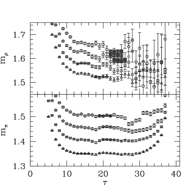
Figure 2: The single pseudo-scalar (lower) and vector (upper) meson effective mass plot obtained from the meson correlation functions on $8^{3}40$ lattices with $\beta=1.7$. Only the results for one value of $\kappa$ is shown. The bare velocity of light is taken to be $\nu=0.90$. The open triangles, open squares, open pentagons and open hexagons are data for the zero and the lowest three non-zero spatial lattice momenta ($(000)$, $(100)$, $(110)$ and $(111)$), respectively. Grey shaded horizontal bars represent the fitted values, the errors and the fitting ranges of the corresponding energy levels, as explained in the text.

The single pseudo-scalar and vector meson, which will be referred to as pion and rho, correlation functions at zero spatial momentum and three lowest lattice momenta, namely $(100)$, $(110$ and $(111)$ are constructed from the corresponding quark propagators. Conventional effective mass functions are computed from which the single meson energy levels with zero and non-zero momentum are extracted from the effective mass plateaus. The fitting range of the plateau is determined automatically by requiring the minimum of the $\chi^{2}$ per degree of freedom of the fit. Using the anisotropic lattices, we are able to obtain decent effective mass plateaus from the single pion and rho correlation functions. In Fig. 2, the effective mass plateaus for the pion and rho are shown for one of our parameter set, namely $8^{3}40$ lattices with $\beta=1.7$. Points with error bars are the effective mass values from the pion (lower half) and rho (upper half) correlation functions. For simplicity, only data for one particular value of $\kappa$ is shown. The grey shaded horizontal regions represent the final fitted value of the energy. The starting and ending positions of these shaded regions correspond to the fitting ranges. The height and thickness of each of these shaded region designates the fitted value and the corresponding error respectively. It is seen that single meson energy values are obtained with good accuracy, especially for the mass. The fitting quality for other parameter sets is similar. The accuracy of the mass values are so good that we could neglect the errors of these mass values when we perform the error analysis of the scattering length where the errors from the energy shifts $\delta E^{(2)}_{\pi\pi}$ are dominating.

Figure 3: The dispersion relation for the pseudo-scalar meson obtained on $8^{3}40$ lattices with $\beta=1.7$. The bare velocity of light is taken to be $\nu=0.90$. It is seen that the measured dispersion relations agree with the free dispersion relation at small lattice momenta with a slope of $1.06(3)$.

Having obtained the single meson energy levels for zero and non-zero spatial momentum, the dispersion relation of the meson is also at our disposal. The parameter $\nu$, also known as the bare velocity of light, that enters the fermion matrix (1) is determined non-perturbatively using the single pion dispersion relations as described in Ref. [20]. In Fig. 3, we show the single pion dispersion relation obtained at the optimal value of $\nu=0.90$ for $\beta=1.7$, $8^{3}40$ lattices. Points with error bars are the single pion energy levels obtained by fitting the pion effective mass plateaus. All data which correspond to $5$ different values of $\kappa$ are plotted. The straight lines are the linear fits to these data. The optimal value of $\nu$ is such that the slope of these lines are consistent with unity. The optimal value of $\nu$ which corresponds to each parameter set of the simulation is also tabulated in Table 1

Figure 4: The ratio $R(t)$ as a function of $t$ obtained from the two pion correlation functions at zero lattice momentum for $5$ different values of the bare quark mass. The lattice size is $8^{3}40$ and the gauge coupling $\beta=2.2$. The optimal bare velocity of light is taken to be $\nu=0.95$. The straight lines are linear fits according to Eq. (12), from which the energy shifts $\delta E\equiv E^{(2)}_{\pi\pi}-2m_{\pi}$ are extracted for all $5$ values of $\kappa$.

Two pion correlation functions and the ratio ${\mathcal{R}}(t)$ are constructed from products of suitable quark propagators according to Wick’s theorem. Both the Direct and the Cross contributions are included. For the ratio ${\mathcal{R}}(t)$, we obtain good signal for all our data sets. In Fig. 4 we show the ratio ${\mathcal{R}}(t)$ for all five $\kappa$ values as a function of the temporal separation $t$, together with the corresponding linear fit (12) for $\beta=2.2$ on $8^{3}40$ lattices. The fitting range cannot start at a value of $t$ that is too small, particularly in a quenched calculation, as discussed in [25]. The starting and ending positions of the straight lines indicate the appropriate fitting range which minimizes the $\chi^{2}$ per degree of freedom. Here, especially on lattices with larger sizes and better signal, we have tried to enlarge the fitting range as much as possible. But for small lattices, e.g. $4^{3}40$ lattices at $\beta=2.6$, signals only last a few time slices.

Table 2: Extracted values of the single pseudo-scalar, vector meson mass and the energy shift $\delta E^{(2)}_{\pi\pi}$ in the isospin $I=2$ channel obtained from the simulation on $4^{3}40$ lattices, all measured in $a^{-1}_{t}$. Also listed are the values of the quantity $F={a^{(2)}_{0}m^{2}_{\rho}\over m_{\pi}}$ (see Sec. 4 for the discussion) obtained by substituting the value of $\delta E^{(2)}_{\pi\pi}$ into Eq. (4).

$\beta=1.7$, $4^{3}40$ lattices					$\beta=2.2$, $4^{3}40$ lattices
$\kappa$	$m_{\pi}$	$m_{\rho}$	$\stackrel{{\scriptstyle\delta E^{(2)}_{\pi\pi}}}{{{}_{(10^{-4})}}}$	$-F$	$\kappa$	$m_{\pi}$	$m_{\rho}$	$\stackrel{{\scriptstyle\delta E^{(2)}_{\pi\pi}}}{{{}_{(10^{-4})}}}$	$-F$
$.057$	$.4129(6)$	$.512(2)$	$99(3)$	$1.29(3)$	$.059$	$.275(1)$	$.334(2)$	$200(3)$	$1.04(1)$
$.056$	$.4827(6)$	$.570(2)$	$89(3)$	$1.42(3)$	$.058$	$.341(1)$	$.392(2)$	$175(3)$	$1.24(1)$
$.055$	$.5503(5)$	$.629(1)$	$81(3)$	$1.57(4)$	$.057$	$.406(1)$	$.451(1)$	$157(3)$	$1.44(1)$
$.054$	$.6163(5)$	$.689(1)$	$75(3)$	$1.72(4)$	$.056$	$.4700(9)$	$.510(1)$	$143(2)$	$1.66(2)$
$.053$	$.6813(5)$	$.7496(8)$	$69(2)$	$1.88(5)$	$.055$	$.5330(8)$	$.570(1)$	$131(2)$	$1.88(2)$
$\beta=2.4$, $4^{3}40$ lattices					$\beta=2.6$, $4^{3}40$ lattices
$\kappa$	$m_{\pi}$	$m_{\rho}$	$\stackrel{{\scriptstyle\delta E^{(2)}_{\pi\pi}}}{{{}_{(10^{-4})}}}$	$-F$	$\kappa$	$m_{\pi}$	$m_{\rho}$	$\stackrel{{\scriptstyle\delta E^{(2)}_{\pi\pi}}}{{{}_{(10^{-4})}}}$	$-F$
$.062$	$.180(2)$	$.216(3)$	$256(19)$	$0.58(3)$	$.063$	$.215(1)$	$.246(2)$	$143(15)$	$0.45(4)$
$.061$	$.245(1)$	$.276(3)$	$218(17)$	$0.78(4)$	$.062$	$.2701(9)$	$.286(2)$	$135(13)$	$0.56(4)$
$.060$	$.308(1)$	$.336(2)$	$186(18)$	$0.97(6)$	$.061$	$.3261(8)$	$.342(2)$	$125(12)$	$0.73(5)$
$.059$	$.368(1)$	$.395(2)$	$140(10)$	$1.03(5)$	$.060$	$.3821(8)$	$.398(2)$	$116(11)$	$0.89(6)$
$.058$	$.428(1)$	$.453(2)$	$158(21)$	$1.45(12)$	$.059$	$.4380(7)$	$.454(1)$	$107(10)$	$1.06(7)$

Table 3: Same as Fig. 2 but for $6^{3}40$ lattices.

$\beta=1.7$, $6^{3}40$ lattices					$\beta=2.2$, $6^{3}40$ lattices
$\kappa$	$m_{\pi}$	$m_{\rho}$	$\stackrel{{\scriptstyle\delta E^{(2)}_{\pi\pi}}}{{{}_{(10^{-4})}}}$	$-F$	$\kappa$	$m_{\pi}$	$m_{\rho}$	$\stackrel{{\scriptstyle\delta E^{(2)}_{\pi\pi}}}{{{}_{(10^{-4})}}}$	$-F$
$.0585$	$.3029(8)$	$.416(2)$	$43(6)$	$1.32(14)$	$.060$	$.202(1)$	$.294(2)$	$81(6)$	$1.19(7)$
$.0575$	$.3803(7)$	$.477(1)$	$37(5)$	$1.45(15)$	$.059$	$.2751(7)$	$.348(2)$	$66(5)$	$1.33(8)$
$.0565$	$.4472(5)$	$.537(1)$	$32(4)$	$1.62(16)$	$.058$	$.3440(8)$	$.404(1)$	$56(5)$	$1.51(9)$
$.0555$	$.5159(4)$	$.597(1)$	$30(4)$	$1.82(18)$	$.057$	$.4097(7)$	$.461(1)$	$49(5)$	$1.72(12)$
$.0545$	$.5827(4)$	$.657(1)$	$28(4)$	$2.03(20)$	$.056$	$.4737(6)$	$.520(1)$	$43(4)$	$1.91(13)$
$\beta=2.4$, $6^{3}40$ lattices					$\beta=2.6$, $6^{3}40$ lattices
$\kappa$	$m_{\pi}$	$m_{\rho}$	$\stackrel{{\scriptstyle\delta E^{(2)}_{\pi\pi}}}{{{}_{(10^{-4})}}}$	$-F$	$\kappa$	$m_{\pi}$	$m_{\rho}$	$\stackrel{{\scriptstyle\delta E^{(2)}_{\pi\pi}}}{{{}_{(10^{-4})}}}$	$-F$
$.0605$	$.205(1)$	$.267(3)$	$66(21)$	$0.82(20)$	$.0615$	$.199(1)$	$.232(2)$	$130(10)$	$1.09(6)$
$.0595$	$.275(1)$	$.322(2)$	$62(8)$	$1.08(10)$	$.0605$	$.2626(9)$	$.291(1)$	$106(8)$	$1.38(6)$
$.0585$	$.3402(9)$	$.379(1)$	$48(10)$	$1.18(19)$	$.0595$	$.3241(6)$	$.351(1)$	$91(7)$	$1.70(8)$
$.0575$	$.4030(8)$	$.436(1)$	$38(10)$	$1.25(25)$	$.0585$	$.3840(5)$	$.409(2)$	$79(6)$	$2.00(10)$
$.0565$	$.4610(6)$	$.494(2)$	$31(10)$	$1.30(32)$	$.0575$	$.4439(6)$	$.467(1)$	$71(6)$	$2.30(12)$

Table 4: Same as Fig. 2 but for $8^{3}40$ lattices.

$\beta=1.7$, $8^{3}40$ lattices					$\beta=2.2$, $8^{3}40$ lattices
$\kappa$	$m_{\pi}$	$m_{\rho}$	$\stackrel{{\scriptstyle\delta E^{(2)}_{\pi\pi}}}{{{}_{(10^{-4})}}}$	$-F$	$\kappa$	$m_{\pi}$	$m_{\rho}$	$\stackrel{{\scriptstyle\delta E^{(2)}_{\pi\pi}}}{{{}_{(10^{-4})}}}$	$-F$
$.0585$	$.3005(7)$	$.421(2)$	$21(3)$	$1.57(21)$	$.060$	$.2026(7)$	$.279(2)$	$45(9)$	$1.43(23)$
$.0575$	$.3782(6)$	$.481(1)$	$14(2)$	$1.43(13)$	$.059$	$.2758(6)$	$.338(1)$	$37(8)$	$1.66(25)$
$.0565$	$.4495(5)$	$.542(1)$	$13(1)$	$1.62(14)$	$.058$	$.3432(5)$	$.397(1)$	$32(7)$	$1.97(29)$
$.0555$	$.5180(4)$	$.597(1)$	$12(1)$	$1.78(17)$	$.057$	$.4084(4)$	$.4558(6)$	$29(6)$	$2.30(34)$
$.0545$	$.5846(4)$	$.657(1)$	$11(1)$	$1.98(18)$	$.056$	$.4721(4)$	$.5150(6)$	$26(6)$	$2.65(39)$
$\beta=2.4$, $8^{3}40$ lattices					$\beta=2.6$, $8^{3}40$ lattices
$\kappa$	$m_{\pi}$	$m_{\rho}$	$\stackrel{{\scriptstyle\delta E^{(2)}_{\pi\pi}}}{{{}_{(10^{-4})}}}$	$-F$	$\kappa$	$m_{\pi}$	$m_{\rho}$	$\stackrel{{\scriptstyle\delta E^{(2)}_{\pi\pi}}}{{{}_{(10^{-4})}}}$	$-F$
$.0605$	$.1966(7)$	$.256(1)$	$56(6)$	$1.43(11)$	$.0605$	$.1991(5)$	$.2394(9)$	$64(10)$	$1.39(15)$
$.0595$	$.2662(6)$	$.3130(8)$	$42(6)$	$1.59(15)$	$.0595$	$.2652(5)$	$.2988(7)$	$52(7)$	$1.73(15)$
$.0585$	$.3317(5)$	$.3717(6)$	$34(5)$	$1.83(19)$	$.0585$	$.3285(4)$	$.3579(6)$	$42(9)$	$2.03(27)$
$.0575$	$.3950(5)$	$.4303(6)$	$29(4)$	$2.09(20)$	$.0575$	$.3904(3)$	$.4167(6)$	$36(8)$	$2.33(33)$
$.0565$	$.4569(4)$	$.4887(5)$	$25(5)$	$2.34(31)$	$.0565$	$.4513(3)$	$.4753(5)$	$32(7)$	$2.65(39)$

Finally, the extracted values of the single meson energy and the energy shifts are all listed in Table 2,Table 3 and Table 4 for $4^{3}40$, $6^{3}40$ and $8^{3}40$ lattices, respectively.

After obtaining the energy shifts $\delta E^{(2)}_{\pi\pi}$, these values are substituted into Lüscher’s formula to solve for the scattering length $a^{(2)}_{0}$ for all five $\kappa$ values. This is done for lattices of all sizes being simulated and for all values of $\beta$. The results for the quantity $F\equiv a^{(2)}_{0}m^{2}_{\rho}/m_{\pi}$ (see the next section for the reason of this choice) are also listed in Table 2 to Table 4. From these results, attempts are made to perform an extrapolation towards the chiral, infinite volume and zero lattice spacing limit.

4 Extrapolation towards chiral, infinite volume and continuum limits

Since the valance quark mass values being studied are far from the chiral limit, we first try to make the chiral extrapolation at finite volume and finite lattice spacing. This is facilitated by results for the scattering length at $5$ different values of $\kappa$. In the chiral limit, the $\pi\pi$ scattering length in the $I=2$ channel is given by the current algebra result due to S. Weinberg [15]:

$$a^{(2)}_{0}=-{1\over 16\pi}{m_{\pi}\over f^{2}_{\pi}}\;\;,$$ (13)

where $a^{(2)}_{0}$ is the $\pi\pi$ scattering length $a_{0}$ in the $I=2$ channel and $f_{\pi}\sim 93$MeV is the pion decay constant. Chiral Perturbation Theory to one-loop order gives an expression which includes the next-to-leading order contributions [16]. Even the next-next-to-leading order corrections have been calculated within Chiral Perturbation Theory [17]. For a summary of the results in Chiral Perturbation Theory, see Ref. [18] and the references therein. Since the one-loop and two-loop numerical results on the pion-pion scattering length in the $I=2$ channel do not differ from the current algebra value substantially, we will mainly compare with Weinberg’s value. Complication arises in the quenched approximation. In principle, the quenched scattering lengths becomes divergent in the chiral limit [25]. However, these divergent terms only become numerically important when the pion mass is close to zero. For the parameters used in our simulation, these terms seem to be numerically small in the $I=2$ channel and we could not observe this divergence from our data.

In most of the previous lattice calculations [11, 12, 13], both the mass and the decay constant of the pion were calculated on the lattice. Then, the lattice results of $m_{\pi}$ and $f_{\pi}$ were substituted into the current algebra result (13) to obtain a prediction of the scattering length. This is to be compared with the scattering length obtained from Lüscher’s formula. In these studies, some discrepancies between the lattice results and the chiral results was observed [13]. There were also discrepancies between the staggered fermion results and the Wilson fermion results. The major disadvantage of the this procedure is the following: First, it is difficult to make a direct chiral extrapolation towards the chiral limit; Second, the lattice results of the decay constant are usually much less accurate, both statistically and systematically, than the mass values. In fact, most of the discrepancies are due to inaccuracy of the decay constants, as realized already in [13]. In this paper, we propose to use another quantity which has a simpler chiral behavior to compare with the current algebra result (13). This quantity is simply $F=a^{(2)}_{0}m^{2}_{\rho}/m_{\pi}$, which in the chiral limit reads:

$$F\equiv{a^{(2)}_{0}m^{2}_{\rho}\over m_{\pi}}=-{1\over 16\pi}{m^{2}_{\rho}\over f^{2}_{\pi}}\sim-1.3638\;\;,$$ (14)

where the final numerical value is obtained by substituting in the experimental values for $m_{\rho}\sim 770$MeV and $f_{\pi}\sim 93$MeV. Note that both $m_{\rho}$ and $f_{\pi}$ have finite values when approaching the chiral limit. Therefore, the above combination will approach a finite value in the chiral limit. On the lattice, we could extract the scattering length $a^{(2)}_{0}$ from Lüscher’s formula. More importantly, the mass of the pion and the rho meson can be obtained with good accuracy on the lattice. So, the factor $F$ can be calculated on the lattice with good precision without the lattice calculation of $f_{\pi}$. The error of the factor $F$ obtained on the lattice will mainly come from the error of the scattering length $a^{(2)}_{0}$, or equivalently, the energy shift $\delta E^{(2)}_{\pi\pi}$ and nowhere else. Since we have calculated the factor $F$ for $5$ different values of valance quark mass, we could make a chiral extrapolation and extract the result in the chiral limit. Comparisons with Weinberg’s result (14) and the experiment will offer us a cross check among different methods.

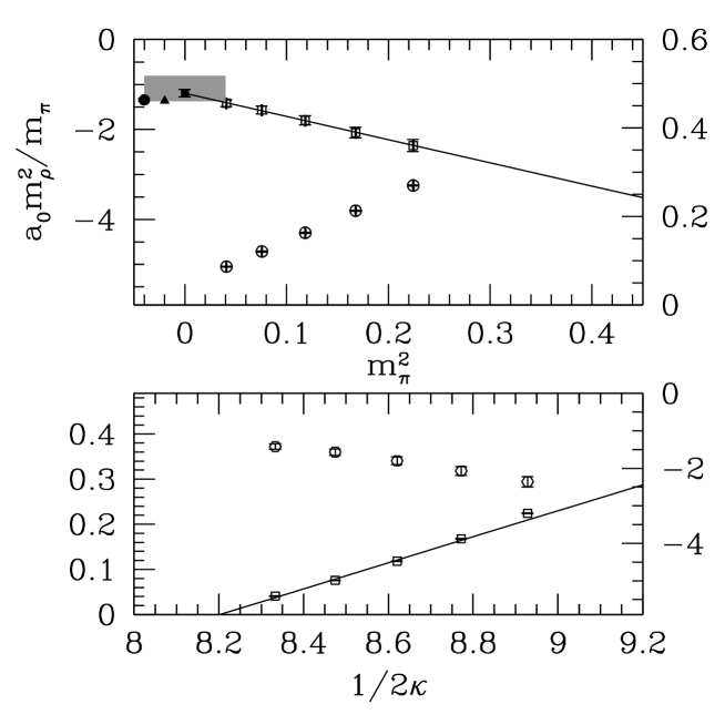
Figure 5: Chiral extrapolation for the quantity $F\equiv a^{(2)}_{0}m^{2}_{\rho}/m_{\pi}$ for our simulation results at $\beta=2.2$ on $6^{3}40$ lattices. In the lower half of the plot, the pseudo-scalar mass squared are plotted as open squares as function of $1/(2\kappa)$. The straight line represents the corresponding linear fit (15) for the data. Also shown in the lower half as open hexagons are the results for the factor $F$. In the upper half of the plot, the same quantity $F$ is plotted (open squares) as a function of $m^{2}_{\pi}$. Also plotted as open circles are the data points for $m^{2}_{\rho}$. The straight line represents the linear extrapolation towards the chiral limit $m^{2}_{\pi}=0$, where the extrapolated result is also depicted as a solid square. As a comparison, the corresponding experimental result [14] for this quantity is drawn as a shaded band. Weinberg’s result and the result from chiral perturbation theory are also shown as a filled triangle and a filled circle at $m_{\pi}=0$, respectively.

In the upper half of Fig. 5, we show the chiral extrapolation of the quantity $F=a^{(2)}_{0}m^{2}_{\rho}/m_{\pi}$ as a function of the pseudo-scalar mass squared ($m^{2}_{\pi}$) for the simulation on $6^{3}40$ lattices at $\beta=2.2$. The open squares represent data points for $F$ at various values of $m^{2}_{\pi}$. The straight line is the linear chiral extrapolation and the extrapolated result is also depicted as a solid square at $m_{\pi}=0$. Weinberg’s result and the result from chiral perturbation theory are also shown as a filled triangle and a filled circle at $m_{\pi}=0$, respectively. The vector meson mass values squared are also shown as the open circles in the upper half of this plot. The pseudo-scalar meson mass squared $m^{2}_{\pi}$ (open squares) are plotted in the lower half of the figure as a function of $1/(2\kappa)$, which linearly depends on the valance quark mass $m_{q}$ via:

$$m_{q}=A\left({1\over 2\kappa}-{1\over 2\kappa_{c}}\right)\;\;,$$ (15)

It is seen that meson mass squared depends on the valance quark mass linearly, as expected from chiral symmetry. It is also possible to dig out the critical value of the hopping parameter where the pseudo-scalar mass vanishes. The data points for the factor $F$ are also shown in the lower half of the plot as open circles. The fitting quality for the pion, rho and the factor $F$ are reasonable. The quality for the chiral extrapolation of other simulation points are similar. As is seen, the linear fit gives a reasonable modeling of the data. The divergent contributions from quenched chiral perturbation theory seem to be numerically small for the lattices being simulated.

Figure 6: Infinite volume extrapolation in Scheme I for the quantity $F=a^{(2)}_{0}m^{2}_{\rho}/m_{\pi}$ for our simulation results at $\beta=2.6$, $2.4$, $2.2$ and $1.7$. The straight lines represent the corresponding linear extrapolation in $1/L^{3}$. The extrapolated result is also shown, together with its error.

Figure 7: Same as Fig. 6 but for Scheme II.

After the chiral extrapolation, we now turn to study the finite volume effects of the simulation. According to formula (4), the quantity $F$ obtained from finite lattices differ from its infinite volume value by corrections of the form $1/L^{3}$. However, it was argued in Ref.[26, 12, 25] that in a quenched calculation, the form of Lüscher’s formula is invalidated. Finite volume corrections will have a different dependence on the volume, e.g. a correction of the form $1/L^{5}$ instead of $1/L^{6}$, as predicted by formula (4). This would mean that the factor $F$ receives finite volume correction of the form $1/L^{2}$. In our simulation, however, we were unable to judge from our data which extrapolation is more convincing. We therefore perform our infinite volume extrapolation in both ways, calling them scheme I ( extrapolating according to $1/L^{3}$ ) and scheme II ( extrapolating according to $1/L^{2}$ ), respectively. In fact, extrapolation in these two different schemes yields compatible results within statistical errors. The fitting quality of Scheme II is somewhat, but not overwhelmingly, better than that of Scheme I. In Fig. 6 and Fig. 7, we have shown the infinite volume extrapolation according to Scheme I and Scheme II, respectively, for the simulation points at $\beta=2.6$, $2.4$, $2.2$ and $1.7$. The extrapolated results are shown with open squares at $L=\infty$, together with the corresponding errors. The straight lines represent the linear extrapolation in $1/L^{3}$ or $1/L^{2}$. It is seen that, on physically small lattices, e.g. those with $\beta=2.6$ and $\beta=2.4$, the finite volume correction is much more significant than larger lattices. For the lattices with $\beta=1.7$, the finite volume dependence of the result is rather weak, showing that even on $4^{3}40$ lattices with this lattice spacing, the finite volume correction is small. This is also reflected by the slopes of the linear fits. It is seen from the figures that the slopes of the fitting straight lines increase with $\beta$, showing a larger finite volume correction at larger $\beta$ values hence smaller lattices.

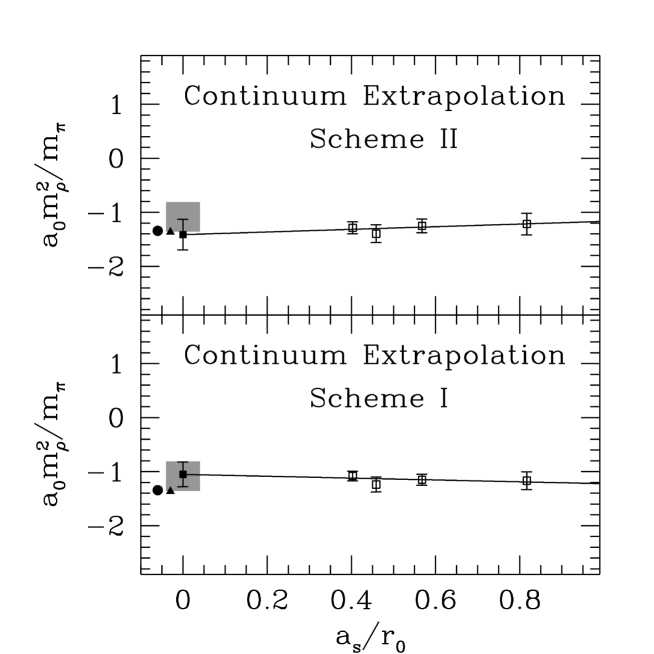
Figure 8: Continuum extrapolation for the quantity $a^{(2)}_{0}m^{2}_{\rho}/m_{\pi}$ obtained from our simulation results at $\beta=2.6$, $2.4$, $2.2$ and $1.7$. The results for both Scheme I and II are shown. The straight lines represent the linear extrapolation in $a_{s}/r_{0}$. The extrapolated results are also shown, together with the experimental result from Ref. [14] indicated by the shaded band. For comparison, Weinberg’s result (14) and the results from Chiral perturbation theory are also shown as the points at $a_{s}=0$ respectively.

Finally, we can make an extrapolation towards the continuum limit by eliminating the finite lattice spacing errors. Since we have used the tadpole improved clover Wilson action, all physical quantities differ from their continuum counterparts by terms that are proportional to $a_{s}$. The physical value of $a_{s}$ for each value of $\beta$ can be found from Ref. [4, 9], which is also included in Table 1. This extrapolation is shown in Fig. 8 where the results from the chiral and infinite volume extrapolation discussed above are indicated as data points in the plot for all $4$ values of $\beta$ that have been simulated. In the lower/upper half of the plot, results in Scheme I/II are shown. The straight lines show the extrapolation towards the $a_{s}=0$ limit and the extrapolated results are also shown as solid squares together with the experimental result from Ref.[14] which is shown as the shaded band. For comparison with chiral perturbation theory, Weinberg’s result (14) and the results from Chiral perturbation theory are also shown as the filled triangles and filled circles at $a_{s}=0$, respectively. It is seen that our lattice calculation gives a compatible result for the quantity $a^{(2)}_{0}m^{2}_{\rho}/m_{\pi}$ when compared with the experiment. The statistical errors for the final result is still somewhat large. This is mainly due to lack of results at smaller lattice spacings. However, the result is promising since the chiral, infinite volume and continxuum extrapolation for the pion scattering length have not been studied systematically using small lattices before. Another encouraging sign is that all data points at different lattice spacing values are about the same which indicates that the $O(a_{s})$ lattice effects are small, presumably due to the tadpole improvement of the action. To summarize, we obtain from the linear extrapolation the following result for the quantity $F=a^{(2)}_{0}m^{2}_{\rho}/m_{\pi}$:

$${a^{(2)}_{0}m^{2}_{\rho}\over m_{\pi}} = -1.05(23)\;\;\mbox{for Scheme I}\;\;,$$

$${a^{(2)}_{0}m^{2}_{\rho}\over m_{\pi}} = -1.41(28)\;\;\mbox{for Scheme II}\;\;.$$ (16)

If we substitute in the mass of the mesons from the experiment: $m_{\rho}\sim 770$MeV and $m_{\pi}\sim 139$MeV, we obtain the quantity $a^{(2)}_{0}m_{\pi}$:

$$a^{(2)}_{0}m_{\pi} = -0.0342(75)\;\;\mbox{for Scheme I}\;\;,$$

$$a^{(2)}_{0}m_{\pi} = -0.0459(91)\;\;\mbox{for Scheme II}\;\;.$$ (17)

Weinberg’s current algebra prediction (13) yields a value of $a^{(2)}_{0}m_{\pi}=-0.046$. This quantity has been calculated in Chiral Perturbation Theory to one-loop order with the result: $a^{(2)}_{0}m_{\pi}=-0.042$ [16] and recently to two-loop order [17, 18]. The final result from Chiral Perturbation Theory gives: $a^{(2)}_{0}m_{\pi}=-0.0444(10)$, where the error comes from theoretical uncertainties. On the experimental side, a new result from E865 collaboration claims $a^{(2)}_{0}m_{\pi}=-0.036(9)$. It is encouraging to find out that our lattice results in both schemes are compatible with the experiment. Our result in Scheme II also agrees with the Chiral Perturbation Theory results very well while our result in Scheme I is barely within one standard deviation of the chiral results.

5 Conclusions

In this paper, we have calculated pion-pion scattering lengths in isospin $I=2$ channel using quenched lattice QCD. It is shown that such a calculation is feasible using relatively small, coarse and anisotropic lattices with limited computer resources like several personal computers and workstations. The calculation is done using the tadpole improved clover Wilson action on anisotropic lattices. Simulations are performed on lattices with various sizes, ranging from $0.8$fm to about $3$fm and with different value of lattice spacing. Quark propagators are measured with $5$ different valance quark mass values. These enable us to explore the finite volume errors and the finite lattice spacing errors in a more systematic fashion. The infinite volume extrapolation is explored in two different schemes which yields compatible final results. The lattice result for the scattering length is extrapolated towards the chiral and continuum limit where a result consistent with the experiment and the Chiral Perturbation Theory is found. We believe that, using the method described in this exploratory study, more reliable and accurate results on pion scattering lengths could be obtained with simulations on larger lattices and computers.

Finally, our method for calculating the pion-pion scattering length discussed in this paper can easily be generalized to calculate the scattering lengths of other hadrons, or in other channels, e.g. $I=0$ channel, where extra care has to be taken due to enhanced terms coming from quenched chiral loops. The method can also be applied to calculate the scattering phase shift at non-zero spatial lattice momenta, where presumably lattices larger than the ones utilized in this exploratory study is needed.

References

- [1] G. P. Lepage and P. B. Mackenzie. Phys. Rev. D, 48:2250, 1993.
- [2] M. Alford, W. Dimm, G. P. Lepage, G. Hockney, and P. B. Mackenzie. Phys. Lett. B, 361:87, 1995.
- [3] C. Morningstar and M. Peardon. Phys. Rev. D, 56:4043, 1997.
- [4] C. Morningstar and M. Peardon. Phys. Rev. D, 60:034509, 1999.
- [5] C. Liu. Chinese Physics Letter, 18:187, 2001.
- [6] C. Liu. Communications in Theoretical Physics, 35:288, 2001.
- [7] C. Liu. In Proceedings of International Workshop on Nonperturbative Methods and Lattice QCD, page 57. World Scientific, Singapore, 2001.
- [8] C. Liu and J. P. Ma. In Proceedings of International Workshop on Nonperturbative Methods and Lattice QCD, page 65. World Scientific, Singapore, 2001.
- [9] C. Liu. Nucl. Phys. (Proc. Suppl.) B, 94:255, 2001.
- [10] C. Liu, Junhua Zhang, Y. Chen, and J.P. Ma. Phys. Lett. B, submitted:hep–lat/0109010, 2001.
- [11] R. Gupta, A. Patel, and S. Sharpe. Phys. Rev. D, 48:388, 1993.
- [12] M. Fukugita, Y. Kuramashi, H. Mino, M. Okawa, and A. Ukawa. Phys. Rev. D, 52:3003, 1995.
- [13] S. Aoki et al. Nucl. Phys. (Proc. Suppl.) B, 83:241, 2000.
- [14] P. Truöl. hep-ex/0012012, 2000.
- [15] S. Weinberg. Phys. Rev. Lett., 17:616, 1966.
- [16] J. Gasser and H. Leutwyler. Phys. Lett. B, 125:325, 1983.
- [17] J. Bijnens et al. Nucl. Phys. B, 508:263, 1997.
- [18] G. Colangelo, J. Gasser, and H. Leutwyler. Nucl. Phys. B, 603:125, 2001.
- [19] T. R. Klassen. Nucl. Phys. (Proc. Suppl.) B, 73:918, 1999.
- [20] Junhua Zhang and C. Liu. Mod. Phys. Lett. A, accepted:hep–lat/0107005, 2001.
- [21] A. Frommer, S. Güsken, T. Lippert, B. Nöckel, and K. Schilling. Int. J. Mod. Phys. C, 6:627, 1995.
- [22] U. Glaessner, S. Guesken, T. Lippert, G. Ritzenhoefer, K. Schilling, and A. Frommer. hep-lat/9605008.
- [23] B. Jegerlehner. hep-lat/9612014.
- [24] M. Lüscher. Commun. Math. Phys., 105:153, 1986.
- [25] C. W. Bernard and M. F. L. Golterman. Phys. Rev. D, 53:476, 1996.
- [26] S. R. Sharpe, R. Gupta, and G. W. Kilcup. Nucl. Phys. B, 383:309, 1992.