Atomic Bose Condensation and the Lattice

Abstract

I show how interaction corrections to the Bose condensation temperature of an atomic gas can be computed using a combination of perturbative effective field theory and lattice techniques.

1 Introduction

This is a lattice talk, but at first it won’t seem like it; it will be about atomic systems, and effective field theories. But studying the effective description of the atomic system will lead to a question suited to lattice techniques. I am summarizing 3 papers [1, 2, 3], all with Peter Arnold; the middle one contains all the lattice stuff.

Many systems exhibit Bose condensation; for instance, liquid Helium, Cooper pairs in superconductors, and arguably nucleon Cooper pairs in large nuclei. These examples condense because of interactions; none exhibit Bose condensation as originally proposed by Bose and Einstein, where condensation occurs exclusively because the temperature is so low that the only place to store the bosons is in the ground state.

The interest in atomic Bose condensation mainly arises because this is what does happen here; mutual interactions are not that important, the dominant reason for condensation is that there is not enough heat to store the density of atoms present in the excited states. In fact, interactions must be weak in an atomic Bose condensate; otherwise it would condense into a solid.

The beauty of small interactions is it means we can calculate; the coupling is weak enough that perturbatively based “field theorist” techniques, like effective field theories and loopwise expansions, can be used.

The question I will address in this talk is, how do interactions modify the relation between density and the temperature of the Bose condensation transition? For simplicity, and to follow the literature, I consider a homogeneous system. (This also makes the question well posed.) It means that the problem addressed is a little artificial and has less contact with experiment than we would like; but nevertheless since there is already a surprisingly big literature on the problem as posed, it is worth addressing.

2 Effective theories

The right effective description of a trapped atomic gas of bosonic atoms, all in the same spin state, is a second quantized Schrödinger equation:

$${\cal L} = \int d^{3}x\;\Psi^{\dagger}\!\left(i\hbar\,\partial_{t}+\frac{\hbar^{2}}{2m}\nabla^{2}-V(x)\right)\!\Psi\vspace{-0.06in}$$ (1)

$$-\int d^{3}x\,d^{3}y\;V(x,y)\>\Psi^{\dagger}\Psi(x)\,\Psi^{\dagger}\Psi(y)\,.\vspace{-0.1in}$$

The atomic number density is $\Psi^{\dagger}\Psi$, with a subtraction implied so the density vanishes in vacuum. Call this Theory I. Technically, Theory I is already an effective theory, containing no information about atomic structure; it is only valid on length scales larger than the atomic size. Since we are concerned with a dilute system we will be interested in scales large compared with the scattering length, in which case the nonlocal interaction term should be replaced with a local term plus higher dimension corrections. Furthermore we are interested in the behavior at finite temperature, and will only ask about static properties (namely the number density), so we can go to the Matsubara formalism, with Euclidean periodic time. I work in the grand canonical ensemble, so I introduce a chemical potential $\mu$, and because the system is homogeneous, $V(x)$ can be dropped. I will also set $\hbar=1$ from now on. The appropriate effective theory is therefore

$$S_{\rm II} \!\!\!=\!\!\! \int_{0}^{\beta}d\tau\int d^{3}x{\cal L}_{\rm E}\,,$$ (2)

$${\cal L}_{\rm E} \!\!\!\!=\!\!\!\! \Psi^{\dagger}\!\left(\!-\partial_{\tau}-\frac{\nabla^{2}}{2m}-\mu\!\right)\!\Psi+\frac{2\pi a_{\rm sc}}{m}(\Psi^{\dagger}\Psi)^{2}\,,\vspace{-0.1in}$$ (3)

plus high dimension operators. The number density is still $\Psi^{\dagger}\Psi$, with its zero temperature value subtracted. This effective theory requires regularization, and I use $\overline{\rm MS}$ dimensional regularization. $a_{\rm sc}$ is the scattering length; we could derive it by matching to Theory I, but we rather define it to be the coefficient shown. There are also high dimension operators, containing either more fields or derivatives; but at the order of interest they can all be dropped. I will call this Theory II.

Theory II contains three interesting length scales $\lambda$:

1. $\lambda\sim a_{\rm sc}\sim 5{\rm nm}$, where it breaks down;

2. $\lambda\sim\lambda_{\rm T}\equiv\sqrt{2\pi/mT}\sim 100$–$300{\rm nm}$, the thermal scale, where nonzero Matsubara frequencies decouple and the behavior becomes effectively 3D;

3. $\lambda\sim\lambda_{\rm T}^{2}/a_{\rm sc}$, the scale were the behavior becomes strongly coupled.

The physics of Bose condensation is associated with the third scale, where the nonzero Matsubara modes have decoupled and the physics is effectively 3D. Therefore we can write a still simpler effective theory which contains the physics of Bose condensation, which I call Theory III:

$$S_{\rm III} \!\!\!=\!\!\! \int d^{3}x\;{\cal L}_{\rm 3D}\,$$ (4)

$${\cal L}_{\rm 3D} \!\!\!=\!\!\! \frac{1}{2}\phi\!\left(-\nabla^{2}+r\right)\!\phi+\frac{u}{24}(\phi^{2})^{2}\,,\vspace{-0.1in}$$ (5)

with $\phi$ a two component real field (the two components correspond to the real and imaginary parts of $\Psi$). Again there are in principle high dimension terms, but we won’t need them. The possibility of such matching was realized by Baym et. al. [4].

The relation between $\mu$, $a_{\rm sc}$, and $\langle\Psi^{\dagger}\Psi\rangle$ in Theory II and $r$, $u$, and $\langle\phi^{2}\rangle$ in Theory III is determined by matching between the theories. The coupling is weak at $\lambda=\lambda_{\rm T}$, so the matching may be done perturbatively. At tree level, $u=96\pi^{2}a_{\rm sc}/\lambda_{\rm T}^{2}$, $\langle\phi^{2}\rangle=\langle\Psi^{\dagger}\Psi\rangle/m$, and $r=-2m\mu$. The operator $\phi^{2}$ mixes with the identity. A one loop matching calculation of the mixing gives the free theory value for the particle number,

$$n_{\rm free}=\zeta(3/2)\;\lambda_{\rm T}^{-3}\,.\vspace{-0.1in}$$ (6)

To find the $O(a_{\rm sc}/\lambda_{\rm T})$ corrections to the number density, we need to find this mixing to two loops, $r$ to one loop, and the other quantities at tree level. We can do even better, and determine the $O(a_{\rm sc}^{2}/\lambda_{\rm T}^{2})$ corrections, by going to one higher loopwise order in every variable. This is done in [3]. We cannot go further without including high dimension operators, so we will stop at this order.

Besides the matching calculation, we also need the critical values of two quantities in Theory III. At linear order in $a_{\rm sc}$ we need the value of $\langle\phi^{2}\rangle$, evaluated at the critical value $r_{\rm crit}$ (the critical $\mu$). At second order in $a_{\rm sc}$, we also need to know the critical value $r_{\rm crit}$. $r_{\rm crit}$ is also needed to find the total number of atoms in a wide but finite trap [5].

3 The lattice

The values of $\langle\phi^{2}\rangle$ and $r_{\rm crit}$ are nonperturbative. Theory III is the 3-D O(2) model, and its infrared behavior falls in the x-y universality class. The infrared behavior is strongly coupled. Furthermore, the quantities of interest, $\langle\phi^{2}\rangle$ and $r_{\rm crit}$, are not universal. They cannot, to our knowledge, be reliably determined using known analytic techniques (perturbation theory, $\epsilon$ expansion, high temperature expansion, etc.). We turn instead to a lattice determination.

We will refer to the lattice regularization of Theory III as Theory IV. $\phi$, a two component real field, is discretized on a 3D cubic lattice of spacing $a_{\rm latt}$, with action

$$S_{\rm IV}\!\!\! = \!\!\!a_{\rm latt}^{3}\sum{\cal L}_{\rm Latt}\,,$$ (7)

$${\cal L}_{\rm Latt}\!\!\! = \!\!\!\frac{1}{2}\phi_{\rm L}\!\left(-Z_{\phi}\nabla_{\rm L}^{2}+r_{\rm L}\right)\phi_{\rm L}+\frac{u_{\rm L}}{24}(\phi_{\rm L}^{2})^{2}\,.$$ (8)

Relating lattice parameters and Theory III parameters, including $\langle\phi_{\rm L}^{2}\rangle$, requires another matching calculation, which is identical in structure to the matching performed between Theories II and III; it can be done by lattice perturbation theory. In [2] we perform this matching to the same, and in some cases higher, loop order, as we used in matching Theories II and III. The matching is an expansion in $a_{\rm latt}u$, which means we want $a_{\rm latt}$ to be relatively small. However we also want to be deep in the critical scaling regime, requiring a large physical volume. To improve the matching to Theory III we use an improved lattice Laplacian, containing anti-ferromagnetic next-nearest couplings (analogous to using the Symanzik rather than Wilson action in pure glue QCD). This frustrates the cluster algorithm, but the multi-grid algorithm [6] is available and proves quite efficient for Monte-Carlo use.

We determine the critical value $r_{\rm crit}$ by the method of Binder [7], which accelerates the large volume convergence; extrapolation of $r_{\rm crit}$ to infinite volume is well behaved. Our matching procedure leaves linear in $a_{\rm latt}$ errors in $r_{\rm L}$, so this extrapolation is less trivial:

Figure 1: Zero spacing extrapolation for $r_{\rm crit}$.

The result is that, at renormalization point $\overline{\mu}=u/3$, $r_{\rm crit}/u^{2}=0.0019201(21)$ [2].

For $\langle\phi^{2}\rangle$ the large volume extrapolation is tougher, and requires a careful accounting of the expected critical behavior. However, the matching has eliminated more of the lattice spacing correction, see Fig. 2. After a double extrapolation, we find $\langle\phi^{2}_{\rm 3D}\rangle/u=-0.001198(17)$ [2].

Putting these results together with the results of the matching calculation between Theory II and Theory III, we determine the correction to $T_{\rm c}$, at fixed number density $n$, to second order in the scattering length. Defining $\rho=a_{\rm scatt}n^{1/3}$,

$$T_{\rm c}\!\!\! = \!\!\!T_{0}\left(1+c_{1}\rho+\left(c_{2}^{\prime}\ln(\rho)+c_{2}^{\prime\prime}\right)\rho^{2}\right)\,,$$ (9)

$$c_{1}\!\!\! = \!\!\!1.32(2)\,,\quad c_{2}^{\prime}=19.75\,,\quad c_{2}^{\prime\prime}=75.7(4)\,,$$ (10)

where $T_{0}$ is determined by inverting Eq. (6).

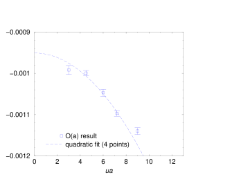
Figure 2: Top: volume behavior, fixed $a_{\rm latt}$. Bottom: $a_{\rm latt}$ behavior, fixed volume.

References

- [1] P. Arnold and G. D. Moore, Phys. Rev. Lett. 87, 120401 (2001), cond-mat/0103228.
- [2] P. Arnold and G. D. Moore, Phys. Rev. E, in production, cond-mat/0103227.
- [3] P. Arnold, G. D. Moore and B. Tomasik, cond-mat/0107124.
- [4] G. Baym, J. Blaizot, M. Holzmann, F. Laloe and D. Vautherin, Phys. Rev. Lett. 83, 1703 (1999), cond-mat/9905430.
- [5] P. Arnold and B. Tomasik, cond-mat/0105147.
- [6] J. Goodman and A. D. Sokal, Phys. Rev. Lett. 56, 1015 (1986).
- [7] K. Binder, Phys. Rev. Lett. 47, 693 (1981); Z. Phys. B 43 (1981) 119.