Deflation of Eigenvalues for GMRES in Lattice QCD

Abstract

Versions of GMRES with deflation of eigenvalues are applied to lattice QCD problems. Approximate eigenvectors corresponding to the smallest eigenvalues are generated at the same time that linear equations are solved. The eigenvectors improve convergence for the linear equations, and they help solve other right-hand sides.

1 Introduction

This paper looks at the iterative solution of complex, non-Hermitian systems of linear equations associated with a lattice QCD problem in particle physics. Let the $n$ by $n$ system of equations be $Ax=b$. We use a version of the GMRES method that deflates eigenvalues and can solve systems with multiple right-hand sides. We give examples that show deflating eigenvalues can make a significant improvement in the convergence for QCD matrices.

We work with the non-Hermitian Wilson-Dirac matrix $M(x,y)$ given by,

$$M(x,y)=I-\kappa\sum_{\mu}[(1+\gamma_{\mu})U_{\mu}^{\dagger}(x-a_{\mu})$$

$$\delta_{x,y+a_{\mu}}+(1-\gamma_{\mu})U_{\mu}(x)\delta_{x,y-a_{\mu}}],$$ (1)

because we perfer to consider systems for which multiple-mass shifts are possible. Our lattice here is of size $12^{3}\times 24$. After the standard even/odd preconditioning, the lattice QCD problem has the form,

$$A_{e}x_{e}=b_{e}+\kappa D_{eo}b_{o},\ \ A_{e}=I-\kappa^{2}D_{eo}D_{oe}.$$ (2)

where $A_{e}$ is of dimension 248,832. We set $\kappa=0.1575$, which for this size matrix and beta value (6.0) means working essentially at $\kappa_{critical}$. We consider a typical, non-exceptional configuration, $U_{\mu}$. The method is designed to efficiently solve the multiple right-hand sides of $Ax=b$ that occur when the “all to all” propagators used for disconnected diagrams are calculated. We will use multiple right-hand sides formed with Z(2) noise vectors. The matrix is not extremely sparse, with about 200 nonzeros per row.

Krylov subspace methods are iterative methods for solving large systems of linear equations. With approximate solution $x_{0}$, and residual vector $r_{0}=b-Ax_{0}$, the linear equations can be recast as $A(x-x_{0})=r_{0}.$ Then the Krylov subspace of dimension $m$ for this problem is $Span\{r_{0},Ar_{0},A^{2}r_{0},...,A^{m-1}r_{0}\}.$ The conjugate gradient method is for Hermitian problems, and GMRES [1, 2] is a well-known Krylov method for the non-Hermitian case.

The effectiveness of Krylov methods is often controlled by the distribution of eigenvalues. The existence of small eigenvalues can significantly slow the convergence rate. This motivates attempts to remove or deflate some eigenvalues from the effective spectrum for an iterative method.

2 The Method

The GMRES method fully orthogonalizes a basis for the Krylov subspace. As the iteration proceeds, the expense and storage both grow. This makes occasional restarting necessary. We refer to each pass through the GMRES iterations between restarts as a “cycle”.

Several approaches have been proposed for deflating eigenvalues from GMRES; see [3] for references. For deflation in QCD problems, see [4, 5, 6, 7]. Our approach differs from previous QCD deflation in that the eigenvalue problem is solved simultaneously with the linear equations.

In this paragraph, we describe the method for the first right-hand side. After the first GMRES cycle, approximate eigenvectors called harmonic Ritz vectors, are computed from the same Krylov subspace generated for solving the linear equations. Let the approximate eigenvectors corresponding to the $k$ approximate eigenvalues of smallest modulus be $\tilde{y}_{1},\tilde{y}_{2},\ldots\tilde{y}_{k}$. For the next cycle, the subspace used for GMRES is

$$Span\{r_{0},Ar_{0},A^{2}r_{0},A^{3}r_{0},\ldots,A^{m-k-1}r_{0},$$

$$\tilde{y}_{1},\tilde{y}_{2},\ldots\tilde{y}_{k}\}.$$ (3)

Having the approximate eigenvectors in the subspace accomplishes two things. The corresponding eigenvalues are deflated once the approximate eigenvectors are moderately accurate. Also the approximate eigenvectors are improved as the method proceeds. It sometimes takes several cycles to improve the approximate eigenvectors to the point that they are useful. This method is called GMRES-DR (GMRES with deflated restarting) [3]. GMRES-DR gives the approximate eigenvectors in the form of a short Arnoldi-type recurrence

$$AV_{k}=V_{k+1}\bar{H}_{k},$$ (4)

where $V_{k}$ is an $n$ by $k$ orthonormal matrix whos columns span the subspace of approximate eigenvectors, and $\bar{H}_{k}$ is a full $k+1$ by $k$ matrix.

Now we look at solving the second and subsequent right-hand sides. We use the eigenvector information that was generated in solving the first right-hand side. An efficient approach in which the eigenvalues are deflated outside of the GMRES cycles with a simple projection is called GMRES-Proj [3]. With the short Arnoldi-type recurrence (4) from GMRES-DR, we need to store only $k+1$ vectors of length $n$ in order to have access to both the approximate eigenvectors and their products with $A$. This allows for fairly inexpensive projections. We use a minimum residual projection [3] here. The GMRES-Proj method applies cycles of standard GMRES, with a projection over the approximate eigenvector subspace in between cycles. This projection is not needed between all of the GMRES cycles.

3 Experiments

We test the approaches just discussed with the matrix $A_{e}$, given earlier.

Example 1. For the first right-hand side, we compare GMRES-DR with standard GMRES. Figure 1 gives a plot of the residual norms for GMRES-DR(40,20), GMRES-DR(20,10), GMRES(40), and GMRES(20). GMRES-DR(40,20) uses subspaces of dimension 40, of which 20 basis vectors are approximate eigenvectors. GMRES(40) also restarts when the subspace reaches dimension 40. Starting around iteration 300, GMRES-DR(40,20) performs considerably better than the other methods. At that point, it has developed good enough approximations to some of the smallest eigenvalues. The eigenvalues halfway surround the origin [8], on the positive real side. This makes the problem difficult, but removing some of the surrounding eigenvalues nearest the origin is helpful.

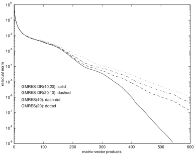
Figure 1: Solution of First Right-hand Side

Example 2. For the second right-hand side, we compare GMRES-Proj with standard GMRES and also with GMRES-DR. With GMRES, there is no deflation, and with GMRES-DR, the deflation happens only after accurate enough approximate eigenvectors develop. Meanwhile, GMRES-Proj is able to deflate from the start. Figure 2 has the residual norms for GMRES(20)-Proj(30), GMRES(20)-Proj(20), GMRES(20)-Proj(10), GMRES(20), and GMRES-DR(40,20). GMRES(20)-Proj(30) refers to cycles of GMRES(20) with occational projections over 30 approximate eigenvectors in between. We project in between every third cycle. GMRES(20)-Proj(20) and GMRES(20)-Proj(10) use the approximate eigenvectors generated while solving the first right-hand side with 400 iterations of GMRES-DR(40,20) and GMRES-DR(20,10), respectively. GMRES(20)-Proj(30)’s eigenvectors come from 610 iterations of GMRES-DR(50,30) (more iterations are needed in this case for the eigenvectors to become accurate enough). The expense per iteration is nearly the same for GMRES(20) and all the GMRES-Proj methods, while GMRES-DR(40,20) has greater orthogonalization expense. More storage is needed for the GMRES-Proj methods than for GMRES. For example, GMRES(20)-Proj(20) needs over 40 vectors of length $n$, while GMRES(20) uses a little over 20. The deflation in GMRES-Proj makes it much better than GMRES(20). GMRES(20)-Proj(20) is also considerably better than GMRES-DR(40,20), because the deflation can start from the beginning (both use 20 Krylov vectors and 20 eigenvectors for each cycle).

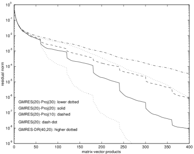
Figure 2: Solution of Second Right-hand Side

4 Conclusion

Deflating eigenvalues is useful for lattice QCD problems, particularly for the second and subsequent right-hand sides. While Z(2) noise vectors were used for these examples, the speedup from deflation is independent of the nature of the right-hand side. Future plans include implementing multiple mass versions of GMRES-DR and GMRES-Proj that solve several systems of equations with shifted matrices but the same right-hand side. We also would like to investigate deflating eigenvalues for the subsequent right-hand sides from Lanczos methods such as the conjugate gradient method and BiCGSTAB.

5 Acknowledgements

The work of both authors is partly supported by the Baylor University Sabbatical Program and NCSA and utilized the SGI Origin 2000 System at the University of Illinois. WW is also partly supported by NSF Grant No. 0070836.

References

- [1] Y. Saad and M. H. Schultz, SIAM J. Sci. Statist. Comput. 7 (1986) 856.
- [2] A. Frommer, Nucl. Phys. B (Proc. Suppl.) 53 (1997) 120.
- [3] R. B. Morgan, “GMRES with Deflated Restarting” Preprint (1999). Available at www.baylor.edu/\̃thinspaceRonald_Morgan.
- [4] P. de Forcrand, Nucl. Phys. B (Proc. Suppl.) 47 (1996) 228.
- [5] R. G. Edwards, U. M. Heller, and R. Narayanan, Phys. Rev. D 59 (1999) 0945101.
- [6] S. J. Dong, F. X. Lee, K. F. Liu, and J. B. Zhang, Phys. Rev. Lett. 85 (2000) 5051.
- [7] H. Neff, N. Eicker, Th. Lippert, J. W. Negele, and K. Schilling, “On the low fermionic eigenmode dominance in QCD on the lattice”, Preprint (2001) hep-lat/0106016.
- [8] B. Medeke. “On Algebraic Multilevel Preconditioners in Lattice Gauge Theory”, A. Frommer et. al. (eds.) Lecture Notes in Comp. Sci. and Eng., Numerical Challenges in Lattice Chromodynamics, Springer, Berlin (2000) p. 99.