Abstract

We discuss hybrid Monte Carlo algorithms for odd-flavor lattice QCD simulations. The algorithms include a polynomial approximation which enables us to simulate odd-flavor QCD in the framework of the hybrid Monte Carlo algorithm. In order to make the algorithms exact, the correction factor to the polynomial approximation is also included in an economical, stochastic way. We test the algorithms for $n_{f}=1$, 1+1 and 2+1 flavors and compare results with other algorithms.

1 Introduction

In lattice QCD simulations the standard algorithm to incorporate effects of dynamical fermions is the Hybrid Monte Carlo (HMC) algorithm [1] which is conventionally used to simulate two-flavor QCD. Due to the algorithmic limitation of the HMC, those simulations are limited to even numbers of degenerate flavors. In order to include dynamical effects correctly, simulations of QCD with three light flavors (u,d,s quarks) are desirable. Simulations with an odd number of flavors can be performed using the R-algorithm [2]. Also for two flavors of staggered fermions [3], the R-algorithm is chosen because the HMC is not applicable. The R-algorithm, however, is not exact: it causes systematic errors of order $(\Delta\tau)^{2}$, where $\Delta\tau$ is the step-size of the Molecular Dynamics evolution. A careful extrapolation to zero step-size is therefore needed to obtain exact results. Nevertheless, it is common practice to forego this extrapolation and to perform simulations with a single step-size chosen small enough that the expected systematic errors are smaller than the statistical ones. In this paper, we wish to emphasize that there is an alternative to the R-algorithm, which gives for our problem arbitrarily accurate results (for infinite computer time) without any extrapolation to $\Delta\tau=0$[4]. Furthermore, we can make our algorithm exact with an additional, stochastic Metropolis test which we describe and implement.

Lüscher proposed a local algorithm, the so-called ”Multiboson algorithm” [5], in which the inverse of the fermion matrix is approximated by a suitable Chebyshev polynomial. Originally he proposed it for two-flavor QCD. Boriçi and de Forcrand [6] noticed that the determinant of a fermion matrix can be written in a manifestly positive way using a polynomial approximation, so that one can simulate odd flavors QCD with the multiboson method. Indeed, using this method, one-flavor QCD was simulated successfully [7]. The same polynomial approximation can be applied for the HMC [8]. The first example of a polynomial approximation within HMC simulations of two-flavor QCD was made by the authors of [8], and later by [9]. Application to odd flavors QCD is straightforward when one uses Boriçi and de Forcrand’s idea. Actually, in the development stage of Ref.[7], one-flavor QCD was also simulated by HMC and it was confirmed that the two algorithmically different methods — multiboson and HMC — give the same distribution of plaquette values [10].

In preliminary work[11], we have simulated $n_{f}=3$ QCD by the HMC with a polynomial approximation, and shown that the results are consistent with those from the R-algorithm. However, the algorithm developed in [11] is not exact yet. A polynomial approximation of moderate degree $n$ may not be sufficiently accurate, especially for small quark masses. For such a case, it is important to control the errors coming from the polynomial approximation. In this study, in order to make our algorithm exact, we include the correction factor to the polynomial approximation into the algorithm and compare our results with those from other algorithms ( R-algorithm with one flavor, and two-flavor HMC ).

A problem specific to odd flavors is the so-called ”sign problem”: the fermionic determinant may change sign configuration by configuration and one has to include the sign into the statistical average (when quarks come in equal-mass pairs, the determinant is squared and its sign does not matter). The calculation of the sign of the determinant on each configuration is feasible in principle, but is very costly. It is common practice to assume that the QCD determinant is always positive. This is the case in the continuum limit, and there are indications that it is also the case for the lattice spacings normally considered and the quark masses currently reachable [12]. Anyway, our goal here is not to study the sign problem, but rather to present an alternative method to the R-algorithm, which samples the absolute value of the determinant like the R-algorithm, but requires no extrapolation.

Our paper is organized as follows. In Sec. 2 we describe the standard HMC algorithm which is used for even-flavor QCD simulations. In Sec. 3 we give our algorithm to simulate odd-flavor QCD, including the additional, stochastic Metropolis step which makes the algorithm exact. In Sec. 4-6 we show results from our algorithm and compare them with other algorithms. We give our conclusions in Sec. 7.

2 Standard Hybrid Monte Carlo Algorithm

The lattice QCD partition function with $n_{f}$ flavors is given by

$$Z=\int[dU](\Pi_{i}^{n_{f}}\det D_{i})\exp(-S_{g}[U]),$$ (1)

where $D_{i}$ is the Wilson Dirac fermion matrix, $D_{i}=1-\kappa_{i}M[U]$ with a hopping parameter $\kappa_{i}$ and $M[U]$ is the lattice Wilson hopping operator. $S_{g}[U]$ stands for the gauge action.

The Hybrid Monte Carlo (HMC) algorithm[1] was developed for a system containing multiples of two degenerate quark flavors. For instance, for $n_{f}=2$ flavors ( two degenerate quarks ), one has the partition function

$$Z=\int[dU]\det D^{2}\exp(-S_{g}[U]).$$ (2)

Using a pseudofermion field $\phi$, an integral representation of the determinant factor $\det D^{2}$ can be given by

$$\det D^{2}\sim\int[d{\phi}^{\dagger}][d{\phi}]\exp(-{\phi}^{\dagger}D^{\dagger-1}D^{-1}\phi),$$ (3)

where the relation, $\det D^{\dagger}=\det D$, is used. The term ${\phi}^{\dagger}{D}^{\dagger-1}{D}^{-1}\phi$ is written in a manifestly positive form which is essential to formulate the HMC algorithm. Introducing momenta $P_{i}$ conjugate to the link variables $U_{i}$, the partition function is rewritten as

$$Z=\int[dU][dP][d{\phi}^{\dagger}][d{\phi}]\exp(-H),$$ (4)

where the Hamiltonian $H$ is defined by

$$H=\frac{1}{2}P^{2}+S_{g}[U]+{\phi}^{\dagger}{D}^{\dagger-1}{D}^{-1}{\phi},$$ (5)

where $P^{2}\equiv\sum_{i}P^{2}_{i}$.

The HMC algorithm consists of two steps: molecular dynamics (MD) evolution and Metropolis accept/reject step. In the MD evolution, one solves Hamilton’s equations of motion:

$$\frac{dU_{i}}{dt} = \frac{\partial H}{\partial P_{i}}$$ (6)

$$\frac{dP_{i}}{dt} = -\frac{\partial H}{\partial U_{i}}.$$ (7)

In general these equations are not solvable analytically. Usually one solves the equations approximately by the 2nd order leapfrog integrator which is time-reversible and area-preserving, thanks to which detailed balance is satisfied. After integrating the equations, one obtains a candidate configuration $(U^{\prime},P^{\prime})$ from the starting configuration $(U,P)$. Next, one performs a Metropolis test with acceptance probability $p=\min(1,\exp(-\delta H))$ where $\delta H=H(U^{\prime},P^{\prime})-H(U,P)$. In case of rejection, one keeps the old $U$. In this study we call the HMC algorithm with Hamiltonian eq.(5) the standard HMC algorithm.

3 Algorithm for Odd Number of Flavors

3.1 $n_{f}=1$ algorithm

The partition function of $n_{f}=1$ QCD is given by

$$Z=\int[dU]\det D\exp(-S_{g}[U]).$$ (8)

In order to simulate $n_{f}=1$ QCD, one has to treat a single $\det D$ which can not be incorporated into the standard HMC. Boriçi and de Forcrand [6] noticed that a single $\det D$, when positive, can be written in a manifestly positive way when Lüscher’s polynomial approximation[5] is used.

One can approximate the inverse of $D$ by a polynomial,

$$1/D\approx P_{m}(D)\equiv\prod_{k=1}^{m}(D-z_{k}),$$ (9)

where $z_{k}$ are the roots of the polynomial $P_{m}(D)$ (a common choice is $z_{k}=1-\exp(i~{}2\pi k/(m+1))$). For a polynomial of even degree $m=2n$, the roots come in complex conjugate pairs $(z_{2k-1},z_{2n+2-2k}),k=1,..,n)$. Thus, eq.(9) is rewritten as

$$P_{2n}(D)=\prod_{k=1}^{n}(D-z_{2k-1})(D-\bar{z}_{2k-1})$$ (10)

where $z_{k}=1-\exp(i~{}2\pi k/(2n+1))$. Using the $\gamma_{5}$ hermiticity of the fermion matrix, one finds that $\det(D-\bar{z}_{k})=\det(D-z_{k})^{\dagger}$. Introducing $T_{n}(D)\equiv\prod_{k=1}^{n}(D-z_{2k-1})$, the determinant of $D$ is written as

$$\det(D)=C_{n}\det(T_{n}^{\dagger}(D)T_{n}(D))^{-1},$$ (11)

with the correction factor $C_{n}$ given by

$$C_{n}\equiv\det(DT_{n}^{\dagger}(D)T_{n}(D))$$ (12)

which goes to one in the limit $n\rightarrow\infty$. An integral representation of $\det(T_{n}^{\dagger}(D)T_{n}(D))^{-1}$ is given by

$$\det(T_{n}^{\dagger}(D)T_{n}(D))^{-1}\sim\int[d\phi^{\dagger}][d\phi]\exp(-\phi^{\dagger}T_{n}^{\dagger}(D)T_{n}(D)\phi).$$ (13)

Note that the term $\phi^{\dagger}T_{n}^{\dagger}(D)T_{n}(D)\phi$ is Hermitian positive, which can not be realized for one flavor in the standard HMC formulation.

Now, the $n_{f}=1$ Hamiltonian for our HMC algorithm can be defined as

$$H^{n_{f}=1}=\frac{1}{2}P^{2}+S_{g}[U]+\phi^{\dagger}T_{n}^{\dagger}(D)T_{n}(D)\phi.$$ (14)

Making use of this Hamiltonian one can perform HMC simulations for $n_{f}=1$ QCD.

The Hamiltonian defined by eq.(14) is an approximation to the exact one, which generates configurations with the measure $\sim\det(T_{n}^{\dagger}(D)T_{n}(D))^{-1}$. The quality of this approximation is measured by the deviation of $C_{n}$ (eq.(12)) from one. To make the algorithm exact, one has to include the correction factor $C_{n}$ into the algorithm. There are several possibilities to incorporate $C_{n}$ in the measure[13]. One possibility is to make a global Metropolis test with probability

$$p=\min\left[1,\frac{C_{n}^{\prime}}{C_{n}}\right],$$ (15)

where $C_{n}^{\prime}\equiv C_{n}[U^{\prime}]$ and $C_{n}\equiv C_{n}[U]$ correspond to a new candidate configuration $U^{\prime}$ and a starting configuration $U$ respectively. Since the correction factor is the determinant of a large matrix, its direct calculation is not feasible. An economical way is to form an unbiased estimator of the ratio ${C_{n}^{\prime}}/{C_{n}}$ and to use a noisy Metropolis test[14, 15]. The same correction factor appears in the $n_{f}=1$ multiboson algorithm[7], where the ratio was estimated by rewriting the correction factor using another high-quality polynomial $T_{r}(D)$ ($r>>n$)[7, 16] as

$$C_{n}=\lim_{r\rightarrow\infty}\frac{\det{T_{n}^{\dagger}(D)T_{n}(D)}}{\det{T_{r}^{\dagger}(D)T_{r}(D)}}.$$ (16)

Using this form of the correction factor, the ratio ${C_{n}^{\prime}}/{C_{n}}$ is written as

$$\frac{C_{n}^{\prime}}{C_{n}} \equiv \det\left[\frac{X^{\prime\dagger}X^{\prime}}{X^{\dagger}X}\right]$$ (17)

$$= \frac{\int d\eta^{\dagger}d\eta\exp(-|X^{\prime-1}X\eta|^{2})}{\int d\eta^{\dagger}d\eta\exp(-|\eta|^{2})}$$

$$= <\exp(-|X^{\prime-1}X\eta|^{2}+|\eta|^{2})>_{\eta}$$

where $X=T_{n}(D)T_{r}(D)^{-1}$. Thus the ratio can be estimated by calculating $\exp(-|X^{\prime-1}X\eta|^{2}+|\eta|^{2})$ with only one Gaussian random vector $\eta$. However convergence is slow, and there may be a technical difficulty using a high-quality polynomial: the above estimation includes a number of ” matrix($D$) $\times$ vector + vector ” type calculations, which results in divergence for high-degree polynomials due to the roundoff errors of computers[11].

We solve this problem very economically here, by proposing to estimate the ratio ${C_{n}^{\prime}}/{C_{n}}$ from unbiased estimators of $({C_{n}^{\prime}}/{C_{n}})^{2}$.

$({C_{n}^{\prime}}/{C_{n}})^{2}$ is easily estimated by

$$\left(\frac{C_{n}^{\prime}}{C_{n}}\right)^{2} = \det\frac{D^{\prime 2}P_{2n}(D^{\prime})^{\dagger}P_{2n}(D^{\prime})}{D^{2}P_{2n}(D)^{\dagger}P_{2n}(D)}=\det\left(\frac{W^{\prime}}{W}\right)^{2}$$ (18)

$$= \frac{\int d\eta^{\dagger}d\eta\exp(-|W^{\prime-1}W\eta|^{2})}{\int d\eta^{\dagger}d\eta\exp(-|\eta|^{2})}$$

$$= <\exp(-|W^{\prime-1}W\eta|^{2}+|\eta|^{2})>_{\eta}$$

where $W\equiv DP_{2n}(D)$. Then the problem is to estimate $({C_{n}^{\prime}}/{C_{n}})$ using unbiased estimators of $({C_{n}^{\prime}}/{C_{n}})^{2}$ only. This can be accomplished by evaluating stochastically the Taylor expansion of $\sqrt{x}$ as shown in [17] for $e^{x}$. Expanding about $x=1$, one writes

$$\sqrt{1+\epsilon}=1+\frac{1}{2}\epsilon+\sum_{k=2}c_{k}(-)^{k-1}\epsilon^{k}$$ (19)

where $c_{k}=\frac{2k-3}{2k}c_{k-1}\in]0,1[$. First, the left-hand side is assigned value 1. Next, with probability $\frac{1}{2}$ one computes a stochastic estimator of $\epsilon_{1}=x-1$ and adds it to the left-hand side. Then, with probability $\frac{2k-3}{2k}c_{k-1}|_{k=2}=\frac{1}{4}$ one computes a second stochastic estimator of $\epsilon_{2}$ and adds $-\epsilon_{1}\epsilon_{2}$ to the left-hand side, and so on. In our case, $x=({C_{n}^{\prime}}/{C_{n}})^{2}$. When the procedure terminates, one obtains an unbiased estimator of $\sqrt{x}$. There is a difficulty if the estimator becomes negative: it cannot be used as a probability in the Metropolis test (eq.(15)). Such positivity violations can be reduced by increasing the degree $n$, to the point where they are never observed during the whole simulation.

Our algorithm is summarized as follows.

1. HMC: we perform Molecular Dynamics with the approximate Hamiltonian eq.(14) and obtain a candidate configuration $U^{\prime}$. Then we do a Metropolis test with acceptance probability $p=\min(1,\exp(-\delta H))$ . This removes the step-size integration error.

2. If the candidate configuration is accepted, we estimate the ratio ${C_{n}^{\prime}}/{C_{n}}$ stochastically by using the method explained above.

3. We perform another Metropolis test with acceptance probability $p=\min(1,\sqrt{x})$, where $\sqrt{x}$ is an unbiased estimator of ${C_{n}^{\prime}}/{C_{n}}$. This removes the error of the polynomial approximation to $\det D$.

4. If accepted, we take $U^{\prime}$ as a new configuration. Otherwise we keep the old configuration.

This algorithm samples the measure $\sqrt{\det^{2}D}=|\det D|$, just like the R-algorithm, but does so in a more efficient way which avoids the extrapolation to zero step-size of the latter. For very small quark masses in the Wilson formulation, the Dirac determinant may become negative for some background gauge fields. This happens for a small fraction of the gauge ensemble, which goes to zero in the continuum limit. Therefore, sampling the measure $|\det D|$ does not affect the continuum limit of the lattice results. Nevertheless, it is possible, if desired, to correct for negative determinants by multiplying the contribution of the corresponding configurations by $-1$ in the Monte Carlo ensemble. This requires identifying possible negative real Dirac eigenvalues in the configurations of that ensemble, which can be done e.g. with the Arnoldi method.

Note that the choice of approximating polynomial is in principle arbitrary: the polynomial approximation error is removed at Step 3 above. However, a poor choice of polynomial, e.g. whose domain of approximation does not cover the complete spectrum of the Dirac operator, will result in difficulty maintaining positivity of the estimator of ${C_{n}^{\prime}}/{C_{n}}$, and in longer autocorrelation times.

3.2 $n_{f}=2+1$ algorithm

The partition function of $n_{f}=2+1$ QCD is given by

$$Z=\int[dU]\det D_{k}^{2}\det D_{l}\exp(-S_{g}[U]).$$ (20)

This system consists of two degenerate quark flavors with a hopping parameter $\kappa_{k}$ and one flavor with $\kappa_{l}$. An integral representation of the determinant factor $\det D_{l}$ is obtained using the polynomial approximation as in eq.(13), whereas $\det D_{k}^{2}$ is expressed as in eq.(3)

$$\det D_{l}\sim{\det}^{-1}(T_{n}^{\dagger}(D_{l})T_{n}(D_{l}))\sim\int[d\phi_{l}^{\dagger}]d\phi_{l}]\exp(-\phi_{l}^{\dagger}T_{n}^{\dagger}(D_{l})T_{n}(D_{l})\phi_{l}),$$ (21)

and

$$\det D_{k}^{2}\sim\int[d{\phi_{k}}^{\dagger}][d{\phi_{k}}]\exp(-\phi_{k}^{\dagger}D_{k}^{\dagger-1}D_{k}^{-1}\phi_{k}).$$ (22)

Combining eq.(21) and (22) one can define the following Hamiltonian,

$$H^{n_{f}=2+1}=\frac{1}{2}P^{2}+S_{g}[U]+\phi_{k}^{\dagger}D_{k}^{\dagger-1}{D_{k}}^{-1}\phi_{k}+\phi_{l}^{\dagger}T_{n}^{\dagger}(D_{l})T_{n}(D_{l})\phi_{l}.$$ (23)

Alternatively, one can express the determinant factors using only one vector $\phi$ as

$$\det D_{k}^{2}\det D_{l}\sim\int[d\phi^{\dagger}][d{\phi}]\exp(-\phi^{\dagger}D_{k}^{\dagger-1}T_{n}^{\dagger}(D_{l})T_{n}(D_{l})D_{k}^{-1}\phi).$$ (24)

Then one obtains another Hamiltonian

$$H^{n_{f}=2+1}=\frac{1}{2}P^{2}+S_{g}[U]+\phi^{\dagger}D_{k}^{\dagger-1}T_{n}^{\dagger}(D_{l})T_{n}(D_{l})D_{k}^{-1}\phi.$$ (25)

Both definitions of Hamiltonian can be used for HMC simulations. In this study we take eq.(23).

The correction factor to the $n_{f}=2+1$ Hamiltonian is given by

$$C_{n}=\det(D_{l}T_{n}^{\dagger}(D_{l})T_{n}(D_{l})).$$ (26)

This factor can be included in the same way as explained for the $n_{f}=1$ algorithm.

3.3 $n_{f}=1+1$ algorithm

The partition function of $n_{f}=1+1$ QCD is given by

$$Z=\int[dU]\det D_{k}\det D_{l}\exp(-S_{g}[U]).$$ (27)

This system consists of two non-degenerate quark flavors with hopping parameters $\kappa_{k}$ and $\kappa_{l}$. Each determinant factor can be expressed in terms of pseudofermion fields using polynomial approximations as

$$\det D_{k}\sim\int[d\phi_{k}][d\phi_{k}^{\dagger}]\exp(-\phi_{k}^{\dagger}T_{n}^{\dagger}(D_{k})T_{n}(D_{k})\phi_{k}),$$ (28)

$$\det D_{l}\sim\int[d\phi_{l}][d\phi_{l}^{\dagger}]\exp(-\phi_{l}^{\dagger}T_{m}^{\dagger}(D_{l})T_{m}(D_{l})\phi_{l}).$$ (29)

Then one defines the $n_{f}=1+1$ Hamiltonian as

$$H^{n_{f}=1+1}=\frac{1}{2}P^{2}+S_{g}[U]+\phi^{\dagger}_{k}T_{n}^{\dagger}(D_{k})T_{n}(D_{k})\phi_{k}+\phi^{\dagger}_{l}T_{m}^{\dagger}(D_{l})T_{m}(D_{l})\phi_{l}$$ (30)

Using one $\phi$ field only, we can express the two determinant factors at once as

$$\det D_{k}\det D_{l}\sim\int[d\phi][d\phi^{\dagger}]\exp(-\phi^{\dagger}T_{n}^{\dagger}(D_{k})T_{m}^{\dagger}(D_{l})T_{m}(D_{l})T_{n}(D_{k})\phi).$$ (31)

This expression results in the following Hamiltonian,

$$H^{n_{f}=1+1}=\frac{1}{2}P^{2}+S_{g}[U]+\phi^{\dagger}T_{n}^{\dagger}(D_{k})T_{m}^{\dagger}(D_{l})T_{m}(D_{l})T_{n}(D_{k})\phi.$$ (32)

In this study we use the definition of eq.(30) for HMC simulations. The correction factor of $n_{f}=1+1$ Hamiltonian is given by

$$C_{nm}\equiv\det\left[D_{k}T_{n}^{\dagger}(D_{k})T_{n}(D_{k})\cdot D_{l}T_{m}^{\dagger}(D_{l})T_{m}(D_{l})\right].$$ (33)

4 Numerical results for $n_{f}=1+1$

We have tested the above algorithms, using relatively small lattices in order to obtain results of sufficient accuracy to expose tiny systematic errors caused by a low-order polynomial approximation or a finite step-size (for the R-algorithm).

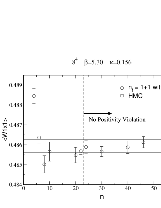
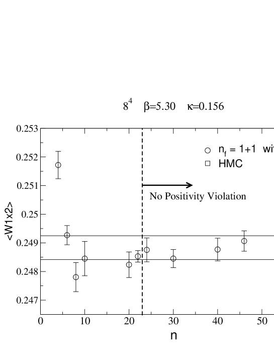
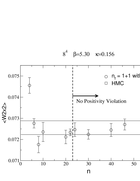
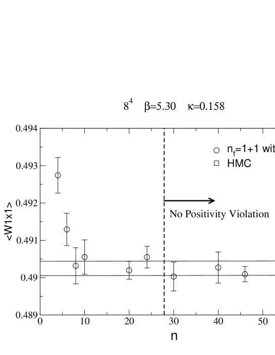
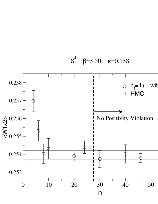
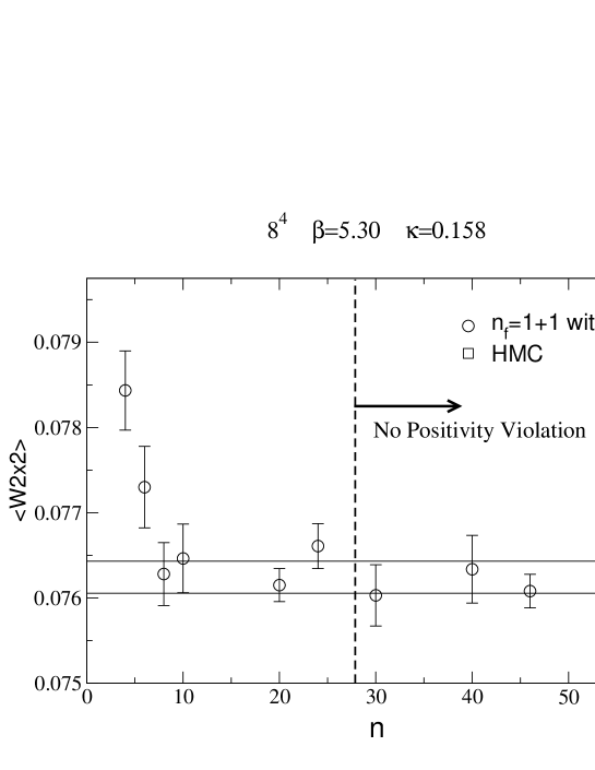
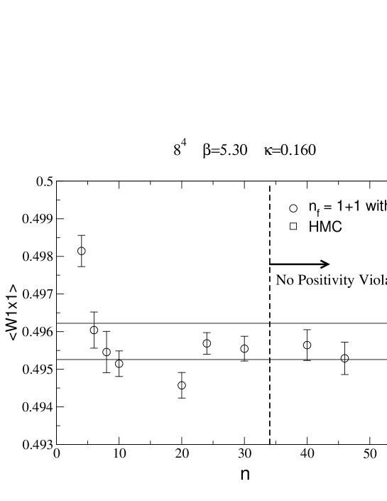
We first show results of $n_{f}=1+1$ QCD with degenerate quark masses. This allows a direct comparison of our results with those of standard $n_{f}=2$ HMC. The algorithm we use here is the one discussed in Sec.3.3, where we set $\kappa\equiv\kappa_{k}=\kappa_{l}$. We use an $8^{4}$ lattice at $\beta=5.30$ and $\kappa=0.156,0.158$ and 0.160. Boundary conditions are anti-periodic in all directions. Since the two quarks have the same mass, we use identical polynomials with the same degree $n$ for the polynomial approximation, ie. $T_{n}(D)=T_{m}(D)$ and $n=m$ and write the correction factor as $C_{n}\equiv C_{nm}$. We measure $1\times 1$, $1\times 2$ and $2\times 2$ Wilson loops and vary the degree $n$ of $T_{n}(D)$. The average values are taken over about 2000-8000 trajectories. Details are shown in Table 1. Average values of Wilson loops are displayed in Figs.1-3 with those from the HMC. Results of Wilson loops are consistent with those from the standard HMC except for small $n$. These results suggest that we do not need to take a very large $n$. Quantitatively, however, from results of Wilson loops only it is not clear which $n$ should be chosen.

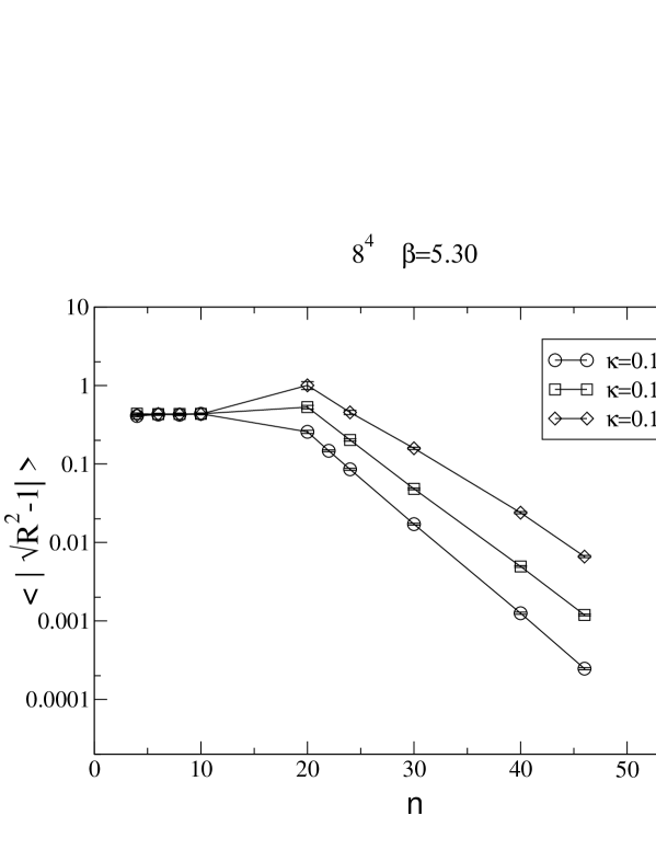
Fig.4 shows the average value of $|C_{n}^{\prime}/C_{n}-1|$ as a function of the degree $n$. Negative values of $C_{n}^{\prime}/C_{n}$ observed for small $n$ are not included in this average. Except for small $n$, $C_{n}^{\prime}/C_{n}$ converges to one exponentially as $n$ increases. The plateau seen at small $n$ is due to the following reason. When the polynomial approximation is inaccurate, i.e. for small $n$, $|W^{\prime-1}W\eta|^{2}$ takes a large value, and the estimated value of $({C_{n}^{\prime}}/{C_{n}})^{2}$ via eq.(18) will always be very small. If we apply eq.(19) with $({C_{n}^{\prime}}/{C_{n}})^{2}=0$ (i.e. $\epsilon=-1$), we obtain $\langle{C_{n}^{\prime}}/{C_{n}}\rangle=0.429$ when the average excludes negative values. This value is consistent with our results. Anyhow we are not interested in such a small $n$ and should increase $n$ until no negative value of $C_{n}^{\prime}/C_{n}$ is observed.

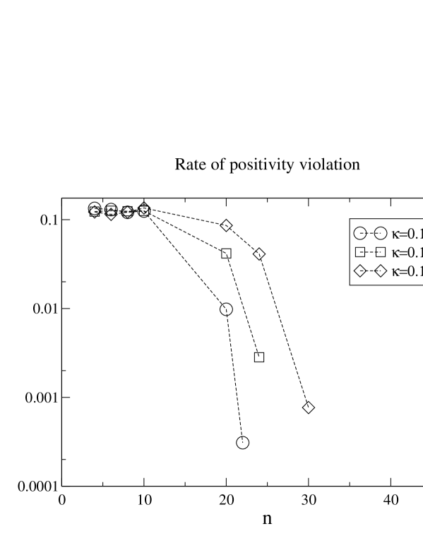
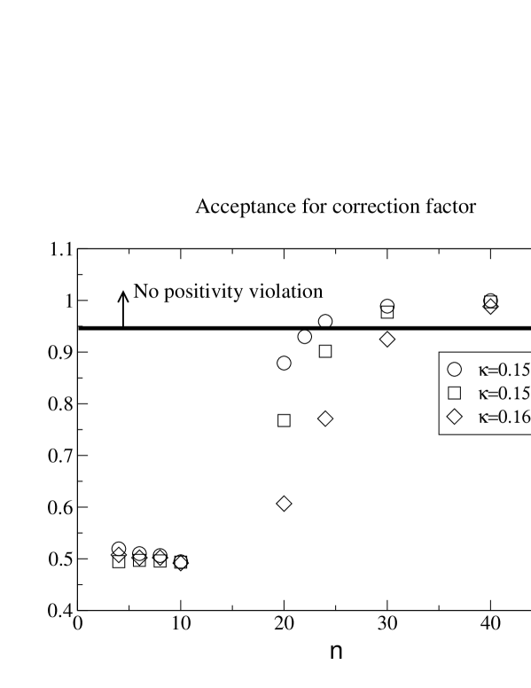
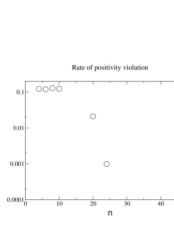
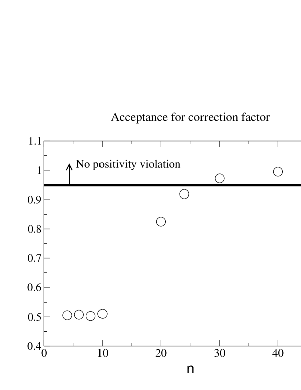
Fig.5 shows the positivity-violation (PV) rate of $C_{n}^{\prime}/C_{n}$. The PV appears to be suppressed exponentially as $n$ increases and one can easily choose the degree $n$ such that no PV would be observed within desired statistics. Within our statistics, no negative value of $C_{n}^{\prime}/C_{n}$ was observed for $n>22$, 24 and 30 at $\kappa=0.156$, 0.158 and 0.160 respectively. However, these values of $n$ will depend on statistics: with high-statistics one may observe a small number of negative values even at large $n$. In order to remove this dependency, let us fix the rate of positivity violation. In this study we are dealing with statistics of $O(10^{3}-10^{4})$ trajectories. So we set the PV level to $10^{-4}$. From Fig.4, roughly speaking, we find that this level corresponds to $n\approx 23,28,34$ for $\kappa=0.156$, 0.158 and 0.160 respectively. The lines indicated by ”No Positivity Violation” in Figs.1-3 correspond to these values of $n$. In turn, as seen in Fig.6, these values of $n$ correspond to an acceptance $\sim 95\%$ in Step 3 of our algorithm. This suggests that typically one needs an acceptance of 95% or higher to maintain positivity of $C_{n}^{\prime}/C_{n}$ at the level of $10^{-4}$. In terms of $C_{n}^{\prime}/C_{n}$, roughly speaking, 95% acceptance corresponds to $<|C_{n}^{\prime}/C_{n}-1|>\approx 0.1$. Under these conditions, the contribution of configurations with negative $C_{n}^{\prime}/C_{n}$ to the total ensemble, if present at all, will be well below the statistical fluctuations, and the way they are dealt with is unimportant. We simply reject such configurations.

5 Numerical results for $n_{f}=1$

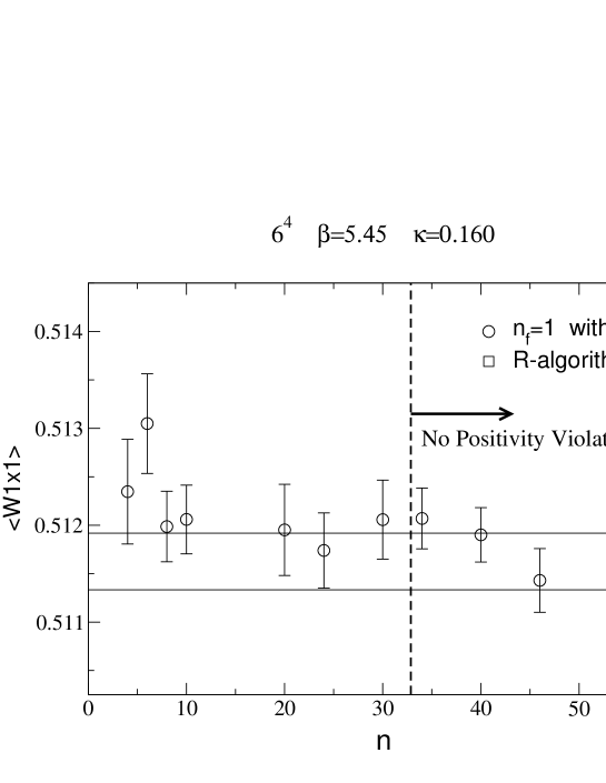
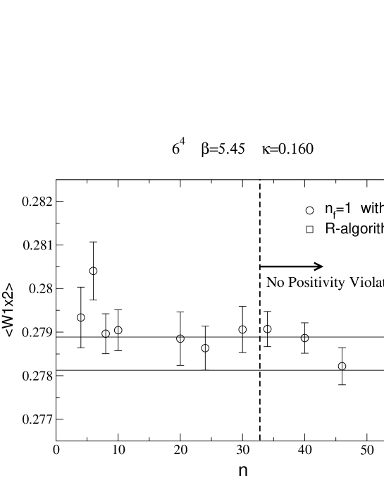
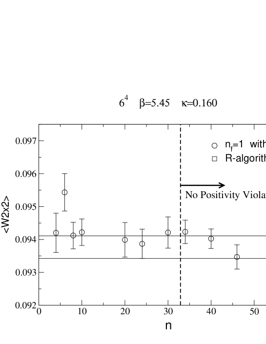
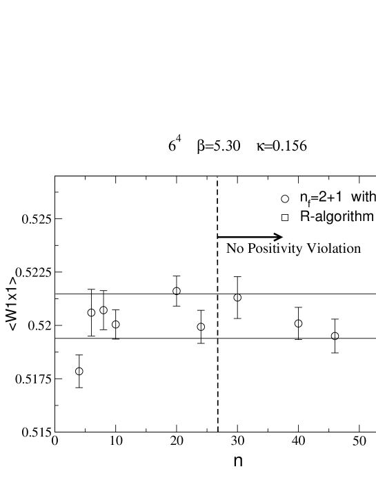
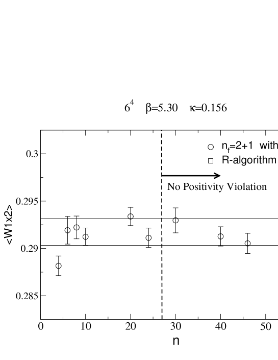
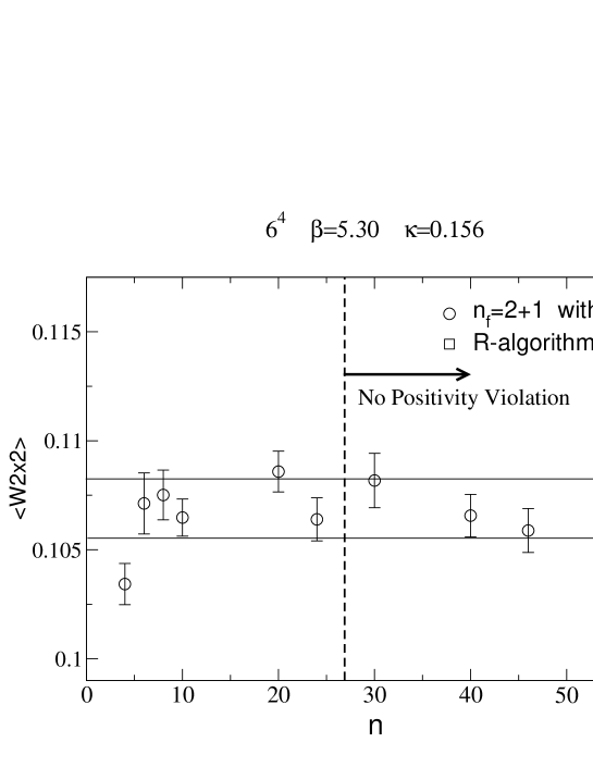
We take a $6^{4}$ lattice at $\beta=5.45$ and $\kappa=0.160$ with periodic boundary conditions in all directions. Simulations are performed using the algorithm of Sec.3.1. Average values of Wilson loops are shown in Fig.7 together with results from the R-algorithm extrapolated to zero step-size. The average values are taken over 10000-36000 trajectories. See Table 3 for details. Our results are consistent with those from the R-algorithm except for small $n$.

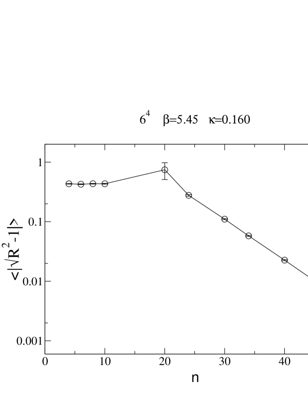
Fig.8 shows the average value of $|C_{n}^{\prime}/C_{n}-1|$. Again, we see exponential convergence as $n$ increases, except for the plateau at small $n$.

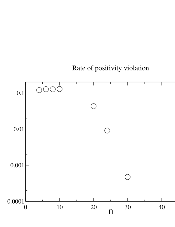
Fig.9 shows the PV rate of $C_{n}^{\prime}/C_{n}$. Positivity violation appears to be suppressed exponentially as $n$ increases. Within our statistics, positivity was maintained for $n>30$. As discussed in Sec.4, adopting a PV level of $10^{-4}$, we find that this level corresponds to $n\approx 33$.

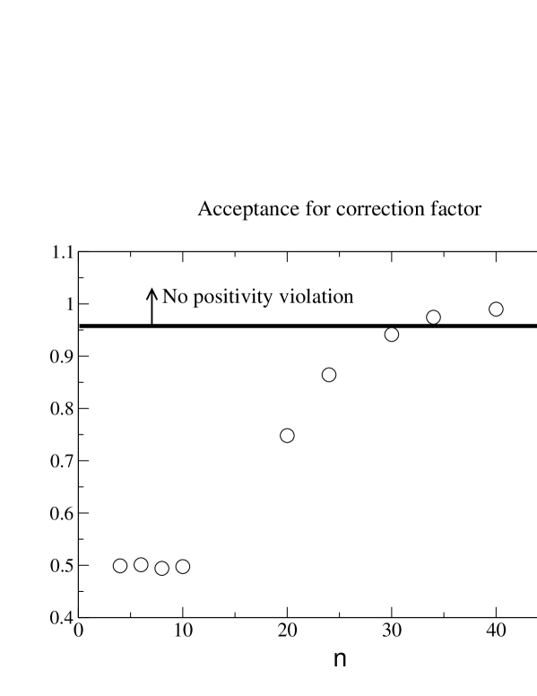
Fig.10 shows the average acceptance of the Metropolis test Step 3. The PV level of $10^{-4}$ corresponds again to about 95% acceptance, and to $<|C_{n}^{\prime}/C_{n}-1|>\approx 0.07$.

6 Numerical results for $n_{f}=2+1$

We take a $6^{4}$ lattice at $\beta=5.30$ and $\kappa=0.156$ with periodic boundary conditions in all directions. Simulations are performed using the algorithm of Sec.3.2. Setting $\kappa\equiv\kappa_{k}=\kappa_{l}$, we can simulate $n_{f}=3$ QCD and compare results with those from $n_{f}=3$ R-algorithm. The average values are taken over 9000-16000 trajectories. See Table 5 for details. Our results are consistent with those from the R-algorithm extrapolated to zero step-size, except for small $n$.

Fig.12 shows the average value of $|C_{n}^{\prime}/C_{n}-1|$. Again we observe exponential convergence as $n$ increases, except for small $n$.

Fig.13 shows the positivity-violation (PV) rate of $C_{n}^{\prime}/C_{n}$. Within our statistics, positivity was maintained for $n>24$. As discussed in Sec.4, adopting a PV level of $10^{-4}$, we find that this level corresponds to $n\approx 27$.

Fig.14 shows the average acceptance of the Metropolis test Step 3. A PV level of $10^{-4}$ corresponds to about 95% acceptance and to $<|C_{n}^{\prime}/C_{n}-1|>\approx 0.1$.

7 Conclusions

We have discussed HMC algorithms for odd-flavor QCD simulations, based on a polynomial approximation of the inverse Dirac operator $D^{-1}$. The algorithms can be made exact with a correction factor which can be easily incorporated in an additional, stochastic Metropolis test. We have tested the algorithms for $n_{f}=1,1+1$ and 2+1 flavors. The results are consistent with those from the standard HMC and R-algorithm.

The estimator of the correction factor $C_{n}^{\prime}/C_{n}$ should be positive if it is to be used in a Metropolis test. We observe that positivity violation is suppressed exponentially as $n$ increases. Therefore, one can choose in advance a value of $n$ which will suffice to avoid negative correction factors in the simulation for the desired statistics. When one fixes the positivity-violation level to $10^{-4}$, this corresponds to about $<|C_{n}^{\prime}/C_{n}-1|>\approx 0.07-0.1$. Equivalently, this level corresponds to $\approx 95\%$ acceptance in the Metropolis test with $p=\min(1,C_{n}^{\prime}/C_{n})$.

Table 1: Step-size $\Delta\tau$, number of trajectories and acceptances for $n_{f}=1+1$ QCD simulations on an $8^{4}$ lattice at $\beta=5.30$. Acc.(HMC) stands for the acceptance with $p=\min(1,\exp(-\delta H))$ which corrects the integration step-size error, and Acc.(CF) is the acceptance from the correction factor with $p=\min(1,C_{n}^{\prime}/C_{n})$, which corrects the error of the polynomial approximation.

$\kappa$	$n$	$\Delta\tau$	trajectories	Acc.(HMC)%	Acc.(CF)%
0.156	4	0.05	3000	78	52
	6	0.05	3000	80	51
	8	0.05	3000	80	51
	10	0.05	4500	80	49
	20	0.05	3000	81	88
	22	0.05	4000	81	93
	24	0.05	3000	80	96
	30	0.05	4000	81	98.9
	40	0.05	4200	82	100
	46	0.05	3600	80	100
0.158	4	0.05	3000	78	49
	6	0.05	4500	77	50
	8	0.05	3000	80	50
	10	0.05	4500	80	49
	20	0.05	5000	81	77
	24	0.05	4000	80	90
	30	0.05	4000	80	98
	40	0.05	4900	80	99.7
	46	0.05	4500	80	99.9
0.160	4	0.05	5000	78	51
	6	0.05	4000	79	50
	8	0.05	7500	80	50
	10	0.05	4500	80	49
	20	0.05	6000	79	61
	24	0.05	3600	80	77
	30	0.05	3200	81	92
	40	0.05	2800	81	98.8
	46	0.05	3000	81	99.7

Table 2: $n_{f}=1+1$ simulation results for $1\times 1$, $1\times 2$ and $2\times 2$ Wilson loops on an $8^{4}$ lattice at $\beta=5.30$.

$\kappa$	$n$	$1\times 1$	$1\times 2$	$2\times 2$
0.156	4	0.48846(37)	0.25172(48)	0.07455(37)
	6	0.48637(28)	0.24927(34)	0.07276(22)
	8	0.48502(44)	0.24780(51)	0.07176(39)
	10	0.48566(48)	0.24845(60)	0.07235(45)
	20	0.48548(39)	0.24824(45)	0.07212(32)
	22	0.48568(16)	0.24853(20)	0.07234(16)
	24	0.48589(34)	0.24876(42)	0.07246(32)
	30	0.48566(25)	0.24845(31)	0.07224(23)
	40	0.48587(31)	0.24877(40)	0.07245(31)
	46	0.48613(28)	0.24906(36)	0.07271(26)
	HMC	0.48594(33)	0.24883(41)	0.07256(32)
0.158	4	0.49274(48)	0.25698(58)	0.07843(46)
	6	0.49129(44)	0.25531(57)	0.07730(48)
	8	0.49032(48)	0.25403(55)	0.07628(37)
	10	0.49055(46)	0.25431(57)	0.07646(40)
	20	0.49020(24)	0.25391(28)	0.07615(19)
	24	0.49055(29)	0.25439(35)	0.07661(26)
	30	0.49003(39)	0.25373(47)	0.07603(36)
	40	0.49027(42)	0.25401(52)	0.07634(40)
	46	0.49009(21)	0.25378(25)	0.07608(20)
	HMC	0.49026(20)	0.25397(25)	0.07624(19)
0.160	4	0.49814(42)	0.26347(52)	0.08326(42)
	6	0.49604(48)	0.26110(61)	0.08180(49)
	8	0.49546(55)	0.26030(69)	0.08102(54)
	10	0.49515(34)	0.25982(45)	0.08054(40)
	20	0.49457(34)	0.25923(42)	0.08016(34)
	24	0.49569(29)	0.26055(35)	0.08120(30)
	30	0.49555(33)	0.26038(49)	0.08102(34)
	40	0.49564(41)	0.26051(51)	0.08106(40)
	46	0.49529(43)	0.26014(55)	0.08089(42)
	HMC	0.49573(48)	0.26068(62)	0.08131(49)

Table 3: Same as in table 1, but for $n_{f}=1$ QCD simulations on a $6^{4}$ lattice at $\beta=5.45$.

$\kappa$	$n$	$\Delta\tau$	trajectories	Acc.(HMC)%	Acc.(CF)%
0.160	2	0.04	5000	93	49
	4	0.04	22000	93	50
	6	0.04	36000	92	50
	8	0.04	20000	93	49
	10	0.05	15000	89	50
	20	0.04	14000	93	75
	24	0.04	10500	93	86
	30	0.04	14300	93	94
	34	0.05	16500	89	97
	40	0.05	15000	89	99
	46	0.05	22000	89	99.4

Table 4: $n_{f}=1$ simulation results for $1\times 1$, $1\times 2$ and $2\times 2$ Wilson loops on a $6^{4}$ lattice at $\beta=5.45$. Results from the R-algorithm were extrapolated to step-size $\Delta\tau=0$, based on simulation results at $\Delta\tau=0.0125$, 0.025, 0.0333333 and 0.04.

$\kappa$	$n$	$1\times 1$	$1\times 2$	$2\times 2$
0.160	2	0.49637(60)	0.25899(73)	0.07794(59)
	4	0.51235(54)	0.27934(70)	0.09420(60)
	6	0.51305(51)	0.28041(67)	0.09543(57)
	8	0.51199(36)	0.27896(46)	0.09412(40)
	10	0.51206(36)	0.27904(47)	0.09422(40)
	20	0.51195(47)	0.27885(61)	0.09399(53)
	24	0.51174(39)	0.27863(51)	0.09387(45)
	30	0.51206(41)	0.27906(53)	0.09421(47)
	34	0.51207(31)	0.27907(40)	0.09423(36)
	40	0.51190(28)	0.27886(35)	0.09402(30)
	46	0.51143(33)	0.27822(43)	0.09347(37)
	R-algorithm	0.51163(29)	0.27850(38)	0.09377(35)

Table 5: Same as in table 1 but for $n_{f}=2+1$ QCD simulations on a $6^{4}$ lattice at $\beta=5.30$.

$\kappa$	$n$	$\Delta\tau$	trajectories	Acc.(HMC)%	Acc.(CF)%
0.156	2	1/18	9000	80	50
	4	1/18	12100	80	51
	6	1/18	15700	81	51
	8	1/18	12000	80	50
	10	1/18	9000	79	51
	20	1/18	12500	81	82
	24	1/18	10000	81	92
	30	1/18	12500	81	97
	40	1/18	14000	81	99.5
	46	1/18	16000	80	99.9

Table 6: $n_{f}=2+1$ simulation results for $1\times 1$, $1\times 2$ and $2\times 2$ Wilson loops on a $6^{4}$ lattice at $\beta=5.30$. Results from the R-algorithm were extrapolated to step-size $\Delta\tau=0$, based on simulation results at $\Delta\tau=0.0125$, 0.0333333, 0.04 and 0.05.

$\kappa$	$n$	$1\times 1$	$1\times 2$	$2\times 2$
0.156	2	0.50032(46)	0.26559(58)	0.08444(48)
	4	0.51785(77)	0.2882(10)	0.10343(95)
	6	0.5206(11)	0.2919(15)	0.1071(14)
	8	0.52072(92)	0.2922(12)	0.1075(11)
	10	0.52005(69)	0.29124(92)	0.10648(85)
	20	0.52161(71)	0.29338(97)	0.10859(94)
	24	0.51993(77)	0.2911(10)	0.10639(99)
	30	0.52131(98)	0.2930(13)	0.1082(12)
	40	0.52009(75)	0.2913(10)	0.10657(98)
	46	0.51950(79)	0.2905(11)	0.1059(10)
	R-algorithm	0.5204(10)	0.2917(14)	0.1069(14)

Figure 1: $n_{f}=1+1$ results of Wilson loop on an $8^{4}$ lattice at $\beta=5.30$ and $\kappa=0.156$.

Figure 2: Same as in fig.1 but for $\kappa=0.158$.

Figure 3: Same as in fig.1 but for $\kappa=0.160$.

Figure 4: $|C_{n}^{\prime}/C_{n}-1|$ as a function of degree $n$ for $n_{f}=1+1$ at $\kappa=0.156$, 0.158 and 0.160. $R$ in the figure stands for $C_{n}^{\prime}/C_{n}$. $C_{n}^{\prime}/C_{n}$ are estimated stochastically by eq.(18) and negative values are not used in the average.

Figure 5: Rate of positivity violation of $C_{n}^{\prime}/C_{n}$ for $n_{f}=1+1$ as a function of degree $n$.

Figure 6: Acceptance of the Metropolis test with $p=\min(1,C_{n}^{\prime}/C_{n})$ for $n_{f}=1+1$.

Figure 7: $n_{f}=1$ results of Wilson loop on a $6^{4}$ lattice at $\beta=5.45$ and $\kappa=0.160$.

Figure 8: $|C_{n}^{\prime}/C_{n}-1|$ for $n_{f}=1$ as a function of degree $n$. $R$ in the figure stands for $C_{n}^{\prime}/C_{n}$.

Figure 9: Rate of positivity violation of $C_{n}^{\prime}/C_{n}$ for $n_{f}=1$ as a function of degree $n$.

Figure 10: Acceptance of Metropolis test with $p=\min(1,C_{n}^{\prime}/C_{n})$ for $n_{f}=1$.

Figure 11: $n_{f}=2+1$ results of Wilson loop on a $6^{4}$ lattice at $\beta=5.30$ and $\kappa=0.156$.

Figure 12: $|C_{n}^{\prime}/C_{n}-1|$ for $n_{f}=2+1$ as a function of degree $n$. $R$ in the figure stands for $C_{n}^{\prime}/C_{n}$.

Figure 13: Rate of positivity violation of $C_{n}^{\prime}/C_{n}$ for $n_{f}=2+1$ as a function of degree $n$.

Figure 14: Acceptance of Metropolis test with $p=\min(1,C_{n}^{\prime}/C_{n})$ for $n_{f}=2+1$.

References

- [1] S. Duane, A. Kennedy, B. Pendleton and D. Roweth, Phys. Lett. B 195 (1987) 216.
- [2] S. Gottlieb, W. Liu, D. Toussaint, R.L. Renken and R.L. Sugar, Phys. Rev. D 35 (1987) 2531.
- [3] J. Kogut and L. Susskind, Phys. Rev. D 11 (1975) 395; L. Susskind, Phys. Rev. D 16 (1977) 3031
- [4] For yet another approach, see T. Lippert, hep-lat/0007029, Lect.Notes Comput.Sci. and Eng. 15 (2000) 166-177.
- [5] M. Lüscher, Nucl. Phys. B 418 (1994) 637; B. Bunk, K. Jansen, B. Jegerlehner, M. Lüscher, H. Simma and R. Sommer, Nucl. Phys. B(Proc.Suppl.) 42 (1995) 49.
- [6] A. Boriçi and Ph. de Forcrand, Nucl. Phys. B 454 (1995) 645.
- [7] C. Alexandrou, A. Boriçi, A. Feo, Ph. de Forcrand, A. Galli, F. Jegerlehner and T. Takaishi, Nucl. Phys. B(Proc.Suppl.) 53 (1997) 435; Nucl. Phys. B(Proc.Suppl.) 63 (1998) 406; Phys. Rev. D 60 (1999) 034504.
- [8] Ph. de Forcrand and T. Takaishi Nucl. Phys. B(Proc.Suppl.) 53 (1997) 968.
- [9] R. Frezzotti and K. Jansen, Phys. Lett. B 402 (1997) 328.
- [10] C. Alexandrou, A. Boriçi, A. Feo, Ph. de Forcrand, A. Galli, F. Jegerlehner and T. Takaishi, 1996, unpublished.
- [11] T. Takaishi, in Proceedings of ”TMU-Yale Symposium on Dynamics of Gauge Fields”, Tokyo, Japan 13 - 15 December 1999, edited by A. Chodos, K. Kitazawa, H. Minakata and C.M. Sommerfield, Frontiers Science Series No.33, UAP, p.181; T. Takaishi and Ph. de Forcrand, Proceedings of the International Symposium ”Confinement 2000”, Osaka, Japan 7 - 10 March 2000 edited by H Suganuma , M Fukushima and H Toki (World Scientific), p.383; Proceedings of the International Workshop ”NON-PERTURBATIVE METHODS AND LATTICE QCD”, Guangzhou, China 15 - 20 May 2000, edited by Xiang-Qian Luo and Eric B Gregory (World Scientific), p.112, hep-lat/0009024; Nucl. Phys. B(Proc.Suppl.) 94 (2001) 818, hep-lat/0011003.
- [12] F. Farchioni, C. Gebert, I. Montvay and W. Schroers, hep-lat/0110130,
- [13] e.g. see for a review, Ph. de Forcrand, hep-lat/9903035.
- [14] A.D. Kennedy and J. Kuti, Phys. Rev. Lett. 54 (1985) 2473.
- [15] G. Bhanot, A.D. Kennedy, Phys. Lett. B 175 (1985) 70.
- [16] I. Montvay, Nucl. Phys. B 466 (1996) 259.
- [17] L. Lin, K.F. Liu and J. Sloan, Phys. Rev. D 61 (2000) 074505.
- [18] C. Alexandrou, A. Borrelli, Ph. de Forcrand, A. Galli and F. Jegerlehner, Nucl. Phys. B 456 (1995) 296.