Tuning the Tadpole Improved Clover Wilson Action on Coarse Anisotropic Lattices

Abstract

Wilson quark action, with tadpole improved clover term added, is studied on coarse anisotropic lattices. The bare velocity of light parameter in this action is determined non-perturbatively using the pseudo-scalar and vector meson dispersion relations for various values of the gauge coupling $\beta$ and bare quark mass parameter $\kappa$.

1 Introduction

It has become clear that anisotropic, coarse lattices and improved lattice actions are the ideal candidates for lattice QCD calculations on small computers [1, 2, 3, 4]. They are particularly advantageous for heavy objects like the glueballs, one meson states with nonzero three momenta and multi-meson states with or without three momenta. The gauge action employed is the tadpole improved gluonic action on asymmetric lattices:

$$S= - \beta\sum_{i>j}\left[{5\over 9}{TrP_{ij}\over\xi u^{4}_{s}}-{1\over 36}{TrR_{ij}\over\xi u^{6}_{s}}-{1\over 36}{TrR_{ji}\over\xi u^{6}_{s}}\right]$$ (1)

$$- \beta\sum_{i}\left[{4\over 9}{\xi TrP_{0i}\over u^{2}_{s}}-{1\over 36}{\xi TrR_{i0}\over u^{4}_{s}}\right]\;\;$$

where $P_{ij}$ is the usual plaquette variable and $R_{ij}$ is the $2\times 1$ Wilson loop on the lattice. The parameter $u_{s}$, which we take to be the $4$-th root of the average spatial plaquette value, incorporates the so-called tadpole improvement and $\xi$ designates the (bare) aspect ratio of the anisotropic lattice.

Using this action, glueball and hadron spectrum has been studied within the quenched approximation [3, 4, 5, 6, 7, 8, 9]. The next step would be to extend the calculation to more complex physical quantities. However, in order to utilize the improved fermionic action [10, 11, 12] on anisotropic lattices, some parameters in the action have to be determined, either perturbatively or non-perturbatively, in order to obtain as much improvement as possible. In this letter, we will discuss the tuning of these parameters in a quenched calculation using clover-improved Wilson fermions on anisotropic lattices. This paper is organized in the following manner. In Section 2, the clover-improved Wilson fermion action on anisotropic lattices is introduced. In Section 3, we focus on the non-perturbative tuning of the bare velocity of light, using the dispersion relations of pseudo-scalar and vector mesons. The optimal values of the bare velocity of light are obtained for various values of $\beta$ and $\kappa$ on different lattices. In Section 4, we will conclude with some general remarks.

2 Improved Wilson Fermions on Asymmetric Lattices

Consider a finite four-dimensional lattice with lattice spacing $a_{\mu}$ along the $\mu$ direction for $\mu=0,1,2,3$. For definiteness, we also denote $a_{0}=a_{t}$ and $a_{i}=a_{s}$ for $i=1,2,3$. We will use $\xi=a_{s}/a_{t}$ to denote the bare aspect ratio of the asymmetric lattice. The un-improved Dirac-Wilson operator on asymmetric lattices is given by:

$$D_{0}={1\over 2}\sum_{\mu}\nu_{\mu}[(\nabla_{\mu}+\nabla^{*}_{\mu})\gamma_{\mu}-a_{\mu}\nabla_{\mu}\nabla^{*}_{\mu}]\;\;,$$ (2)

where $\nabla_{\mu}$ and $\nabla^{*}_{\mu}$ are the usual lattice forward and backward derivatives. The parameter $\nu_{\mu}$ enters the Dirac-Wilson operator since the hyper-cubic symmetry is broken. In particular, we have $\nu_{0}=1$ and $\nu_{i}\equiv\nu$ which we call the “bare” velocity of light. The clover-improved Dirac-Wilson operator is obtained by adding a Scheikholeslami-Wohlert, or clover, term to the usual Wilson fermion action [13]. To implement the tadpole improvement, one replaces each spatial link $U_{i}(x)$ by $U_{i}(x)/u_{s}$ while keeping the temporal link unchanged. In quenched calculations, one usually needs to calculate the quark propagators at various valance quark masses. This amounts to different values of $m_{0}$ or $\kappa$ for the same gauge field configuration. In this case, it is convenient to use the following fermion matrix:

$${\mathcal{M}}_{xy} = \delta_{xy}\sigma+{\mathcal{A}}_{xy}$$

$${\mathcal{A}}_{xy} = \delta_{xy}\left[1/(2\kappa_{max})+\rho_{t}\sum^{3}_{i=1}\sigma_{0i}{\mathcal{F}}_{0i}+\rho_{s}(\sigma_{12}{\mathcal{F}}_{12}+\sigma_{23}{\mathcal{F}}_{23}+\sigma_{31}{\mathcal{F}}_{31})\right]$$ (3)

$$- \sum_{\mu}\eta_{\mu}\left[(1-\gamma_{\mu})U_{\mu}(x)\delta_{x+\mu,y}+(1+\gamma_{\mu})U^{\dagger}_{\mu}(x-\mu)\delta_{x-\mu,y}\right]\;\;,$$

where the coefficients are given by:

$$\eta_{i} = \nu/(2u_{s})\;\;,\;\;\eta_{0}=\xi/2\;\;,\;\;\sigma=1/(2\kappa)-1/(1\kappa_{max})\;\;,$$

$$\rho_{t} = c_{SW}(1+\xi)/(4u^{2}_{s})\;\;,\;\;\rho_{s}=c_{SW}/(2u^{4}_{s})\;\;.$$ (4)

In this notation, the bare quark mass dependence is singled out into the parameter $\sigma$ and the matrix ${\mathcal{A}}$ remains unchanged if the bare quark mass is varied. Therefore, one could utilize the shifted structure of the matrix ${\mathcal{M}}$ to solve for quark propagators at various values of $m_{0}$ (or equivalently $\kappa$) at the cost of solving only one value of $\kappa=\kappa_{max}$, using the so-called Multi-Mass Minimal Residual ($M^{3}R$) algorithm [14, 15, 16].

3 Tuning of the parameters

Tuning the bare parameters of the fermion matrix to obtain the best improvement is a rather delicate issue [11]. In a quenched calculation, the matter is simplified since the anisotropy $\xi$ can be determined from the pure gauge sector. In fact, with the tadpole improvement, the renormalization effects of the aspect ratio can be ignored [3, 4]. The parameter $c_{SW}$ is the hardest to be tuned. In principle, one could utilize the Schrödinger representation of the QCD path integral to determine this parameter non-perturbatively. This has been done for the clover-improved Wilson fermion action on symmetric lattices [17, 18]. In this work, the tadpole improved tree-level value is used. In what follows, we will focus on the tuning of the parameter $\nu$. Since this parameter has rather weak dependence on the quark mass on anisotropic lattices [11], it can be determined non-perturbatively by the pseudo-scalar meson dispersion relation for a rather heavy pion.

Results of this tuning process for various values of $\beta$, together with the corresponding simulation parameters

Table 1: Simulation parameters for $\beta=1.7$ lattices. Input aspect ratio parameter $\xi$ is fixed to be $5$ throughout this paper. The approximate spatial lattice spacing $a_{s}$ in physical units as obtained from [4] is also shown. Results for pion mass, rho mass in lattice units, the slope of the pseudo-scalar and vector meson dispersion relation $Z_{\pi}$ and $Z_{\rho}$ (see Eq. (5) for the definition of them), and the corresponding value of $\nu$ and $\kappa$ are also listed.

$\beta=1.7$, $a_{s}\sim 0.39fm$, $6^{3}40$ lattices
$\nu=0.90$, $288$ configurations					$\nu=0.92$, $192$ configurations
$\kappa$	$m_{\pi}a_{t}$	$m_{\rho}a_{t}$	$Z_{\pi}$	$Z_{\rho}$	$\kappa$	$m_{\pi}a_{t}$	$m_{\rho}a_{t}$	$Z_{\pi}$	$Z_{\rho}$
$.0585$	$0.3029(8)$	$0.416(2)$	$0.97(2)$	$1.01(5)$	$.059$	$0.230(1)$	$0.360(5)$	$0.97(2)$	$1.04(6)$
$.0575$	$0.3803(7)$	$0.477(1)$	$1.06(1)$	$1.08(4)$	$.058$	$0.315(1)$	$0.427(2)$	$1.02(3)$	$1.12(5)$
$.0565$	$0.4472(5)$	$0.537(1)$	$1.09(2)$	$1.15(4)$	$.057$	$0.3916(9)$	$0.491(4)$	$1.11(2)$	$1.19(5)$
$.0555$	$0.5159(4)$	$0.597(1)$	$1.18(1)$	$1.06(4)$	$.056$	$0.4625(8)$	$0.552(3)$	$1.17(2)$	$1.10(7)$
$.0545$	$0.5827(4)$	$0.657(1)$	$1.23(1)$	$1.08(4)$	$.055$	$0.5319(7)$	$0.612(2)$	$1.22(2)$	$1.15(5)$

are given in Table 1 to Table 5. The value of $\beta$ in our simulations ranges between $1.7$ and $3.0$, which roughly corresponds to physical spatial lattice spacing $a_{s}$ in the range $0.12\sim 0.4fm$. The aspect ratios of these lattices are fixed at $\xi_{0}=5$. The spatial sizes of the lattices range from $L=4$ to $L=8$, which in physical units lie in the range $0.5\sim 3.2fm$, depending on the value of $\beta$. For simplicity, only the results for $6^{3}40$ lattices that are close to the optimal value of $\nu$ are shown.

Table 2: Same as Table 1 except for $\beta=2.2$.

$\beta=2.2$, $a_{s}\sim 0.27fm$, $6^{3}40$ lattices
$\nu=0.90$, $160$ configurations					$\nu=0.95$, $208$ configurations
$\kappa$	$m_{\pi}a_{t}$	$m_{\rho}a_{t}$	$Z_{\pi}$	$Z_{\rho}$	$\kappa$	$m_{\pi}a_{t}$	$m_{\rho}a_{t}$	$Z_{\pi}$	$Z_{\rho}$
$.061$	$0.198(1)$	$0.291(3)$	$0.89(4)$	$0.93(6)$	$.060$	$0.203(1)$	$0.294(2)$	$0.99(4)$	$0.98(6)$
$.060$	$0.268(1)$	$0.341(2)$	$0.96(3)$	$1.00(5)$	$.059$	$0.276(1)$	$0.351(2)$	$1.04(3)$	$1.07(5)$
$.059$	$0.3361(7)$	$0.397(2)$	$1.00(3)$	$1.07(4)$	$.058$	$0.3443(6)$	$0.406(2)$	$1.10(2)$	$1.17(4)$
$.058$	$0.3994(5)$	$0.452(2)$	$1.07(2)$	$1.16(4)$	$.057$	$0.4091(5)$	$0.463(1)$	$1.18(2)$	$1.25(4)$
$.057$	$0.4616(5)$	$0.509(1)$	$1.19(2)$	$1.18(5)$	$.055$	$0.4728(4)$	$0.520(1)$	$1.26(2)$	$1.34(3)$

Table 3: Same as Table 1 except for $\beta=2.4$.

$\beta=2.4$, $a_{s}\sim 0.22fm$, $6^{3}40$ lattices
$\nu=0.90$, $192$ configurations					$\nu=0.92$, $192$ configurations
$\kappa$	$m_{\pi}a_{t}$	$m_{\rho}a_{t}$	$Z_{\pi}$	$Z_{\rho}$	$\kappa$	$m_{\pi}a_{t}$	$m_{\rho}a_{t}$	$Z_{\pi}$	$Z_{\rho}$
$.061$	$0.207(1)$	$0.265(3)$	$0.96(3)$	$1.05(5)$	$.0605$	$0.204(1)$	$0.265(3)$	$0.99(3)$	$1.10(6)$
$.060$	$0.2713(9)$	$0.320(2)$	$1.08(2)$	$1.13(4)$	$.0595$	$0.273(1)$	$0.319(2)$	$1.08(3)$	$1.17(4)$
$.059$	$0.3351(8)$	$0.377(1)$	$1.16(2)$	$1.19(3)$	$.0585$	$0.338(1)$	$0.376(2)$	$1.16(3)$	$1.22(4)$
$.058$	$0.3971(7)$	$0.434(1)$	$1.22(2)$	$1.26(3)$	$.0575$	$0.3973(8)$	$0.433(1)$	$1.26(3)$	$1.28(4)$
$.057$	$0.4579(6)$	$0.491(1)$	$1.28(2)$	$1.27(3)$	$.0565$	$0.4587(6)$	$0.491(1)$	$1.31(2)$	$1.31(4)$

Table 4: Same as Table 1 except for $\beta=2.6$.

$\beta=2.6$, $a_{s}\sim 0.19fm$, $6^{3}40$ lattices
$\nu=0.85$, $192$ configurations					$\nu=0.88$, $192$ configurations
$\kappa$	$m_{\pi}a_{t}$	$m_{\rho}a_{t}$	$Z_{\pi}$	$Z_{\rho}$	$\kappa$	$m_{\pi}a_{t}$	$m_{\rho}a_{t}$	$Z_{\pi}$	$Z_{\rho}$
$.062$	$0.206(1)$	$0.243(2)$	$0.99(3)$	$1.08(4)$	$.0615$	$0.199(1)$	$0.236(2)$	$1.02(3)$	$1.09(5)$
$.061$	$0.2687(8)$	$0.301(1)$	$1.07(2)$	$1.16(3)$	$.0605$	$0.2628(8)$	$0.295(2)$	$1.11(2)$	$1.21(3)$
$.060$	$0.3288(6)$	$0.358(1)$	$1.16(2)$	$1.22(3)$	$.0595$	$0.3243(6)$	$0.354(1)$	$1.18(2)$	$1.22(3)$
$.059$	$0.3886(8)$	$0.415(1)$	$1.20(2)$	$1.26(3)$	$.0585$	$0.3852(8)$	$0.411(1)$	$1.25(2)$	$1.32(3)$
$.058$	$0.4468(7)$	$0.471(1)$	$1.25(2)$	$1.30(2)$	$.0575$	$0.4446(7)$	$0.469(1)$	$1.31(2)$	$1.36(3)$

Table 5: Same as Table 1 except for $\beta=3.0$.

$\beta=3.0$, $a_{s}\sim 0.12fm$, $6^{3}40$ lattices
$\nu=0.85$, $192$ configurations					$\nu=0.88$, $192$ configurations
$\kappa$	$m_{\pi}a_{t}$	$m_{\rho}a_{t}$	$Z_{\pi}$	$Z_{\rho}$	$\kappa$	$m_{\pi}a_{t}$	$m_{\rho}a_{t}$	$Z_{\pi}$	$Z_{\rho}$
$.0635$	$0.149(2)$	$0.152(2)$	$1.00(3)$	$0.90(4)$	$.062$	$0.191(1)$	$0.202(2)$	$1.05(2)$	$1.09(3)$
$.0625$	$0.199(1)$	$0.206(2)$	$1.02(2)$	$1.09(3)$	$.061$	$0.246(1)$	$0.258(1)$	$1.14(2)$	$1.16(3)$
$.0615$	$0.253(1)$	$0.262(1)$	$1.10(2)$	$1.16(2)$	$.060$	$0.302(1)$	$0.314(1)$	$1.21(2)$	$1.24(2)$
$.0605$	$0.3086(9)$	$0.318(1)$	$1.17(2)$	$1.22(2)$	$.059$	$0.3593(9)$	$0.371(1)$	$1.20(2)$	$1.29(2)$
$.0595$	$0.3644(8)$	$0.373(1)$	$1.16(2)$	$1.27(2)$	$.058$	$0.4161(8)$	$0.427(1)$	$1.26(2)$	$1.34(2)$

Quark propagators with various three momenta are obtained using the $M^{3}R$ algorithm with wall sources. In this work, only the meson energy for zero and the following three non-zero lattice momenta are measured, namely $(100)$, $(110)$ and $(111)$ with Dirichlet boundary conditions applied in the temporal direction. Then the pseudo-scalar correlation functions and the vector meson correlation functions are constructed, from which the single pion energy and the single rho energy are extracted in lattice units. Due to the advantage of the anisotropic lattices, the meson energy levels can be measured with good accuracy. Errors are obtained using the standard jack-knife method. The mass of the pion and rho, are also listed in Table 3. The single meson energy levels are fitted according to the expected dispersion relation:

$$\omega^{2}_{\pi}({\mathbf{k}})=m^{2}_{\pi}+Z_{\pi}{\mathbf{k}}^{2}\;\;,\;\;\omega^{2}_{\rho}({\mathbf{k}})=m^{2}_{\rho}+Z_{\rho}{\mathbf{k}}^{2}\;\;.$$ (5)

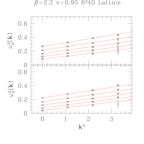
In Fig. 1, the dispersion relations of the pseudo-scalar (the lower plot) and the vector meson (the upper plot) are shown for $\beta=2.2$, $\nu=0.95$ and five different values of $\kappa$ on $6^{3}40$ lattices. The straight lines represent the fits using the first three lowest momentum points (including the zero-momentum point) according to Eq. (5). It is seen that the above dispersion relations fit the simulation data well for lattice momenta that are not too large. Fitting qualities are similar for other parameter sets. The results of the slope obtained from the fitting are also included in Table 3. By tuning the bare velocity of light parameter $\nu$, we obtain a value of $Z_{\pi}$ which is consistent with unity.

Figure 1: The dispersion relation for the pseudo-scalar (the lower plot) and vector meson (the upper plot) obtained on $6^{3}40$ lattices with $\beta=2.2$ at five different pion masses. The bare velocity of light is taken to be $0.95$. It is seen that the measured dispersion relations agree with the free dispersion relation at small lattice momenta.

The same tuning procedure is also applied to smaller ($4^{3}40$) and larger ($8^{3}40$) lattices. The outcome of the procedure is quite similar. No significant dependence of the parameter $\nu$ on the volume of the lattice has been observed.

4 Conclusions

In this letter, we outline the method on the non-perturbative determination of the bare velocity of light parameter $\nu$ in the anisotropic Wilson quark action . The optimal values of $\nu$ are obtained for various values of $\beta$ and $\kappa$. These values can then be utilized in a quenched calculation using the improved anisotropic Wilson action. Some of these calculations are in progress and we hope to report the results soon.

References

• [1] G. P. Lepage and P. B. Mackenzie. Phys. Rev. D, 48:2250, 1993.
• [2] M. Alford, W. Dimm, G. P. Lepage, G. Hockney, and P. B. Mackenzie. Phys. Lett. B, 361:87, 1995.
• [3] C. Morningstar and M. Peardon. Phys. Rev. D, 56:4043, 1997.
• [4] C. Morningstar and M. Peardon. Phys. Rev. D, 60:034509, 1999.
• [5] C. Liu. Chinese Physics Letter, 18:187, 2001.
• [6] C. Liu. Communications in Theoretical Physics, 35:288, 2001.
• [7] C. Liu. In Proceedings of International Workshop on Nonperturbative Methods and Lattice QCD, page 57. World Scientific, Singapore, 2001.
• [8] C. Liu and J. P. Ma. In Proceedings of International Workshop on Nonperturbative Methods and Lattice QCD, page 65. World Scientific, Singapore, 2001.
• [9] C. Liu. Nucl. Phys. (Proc. Suppl.) B, 94:255, 2001.
• [10] M. Alford, T. R. Klassen, and P. Lepage. Nucl. Phys. B, 496:377, 1997.
• [11] T. R. Klassen. Nucl. Phys. (Proc. Suppl.) B, 73:918, 1999.
• [12] S. Aoki, Y. Kuramashi, and S. Tominaga. Relativistic heavy quarks on the lattice. hep-lat/0107009.
• [13] B. Sheikholeslami and R. Wohlert. Nucl. Phys. B, 259:572, 1985.
• [14] A. Frommer, S. GΓΌsken, T. Lippert, B. NΓΆckel, and K. Schilling. Int. J. Mod. Phys. C, 6:627, 1995.
• [15] U. Glaessner, S. Guesken, T. Lippert, G. Ritzenhoefer, K. Schilling, and A. Frommer. How to compute green’s functions for entire mass trajectories within krylov solvers. hep-lat/9605008.
• [16] B. Jegerlehner. Krylov space solvers for shifted linear systems. hep-lat/9612014.
• [17] K. Jansen, C. Liu, et al. Phys. Lett. B, 372:275, 1996.
• [18] K. Jansen and R. Sommer. Nucl. Phys. B, 530:185, 1998.
• [19] H. Matsufuru, T. Onogi, and T. Umeda. Numerical study of $O(a)$ improved wilson quark action on anisotropic lattice. hep-lat/0107001.