Improved Smoothing Algorithms for Lattice Gauge Theory

Abstract

The relative smoothing rates of various gauge field smoothing algorithms are investigated on ${\cal O}(a^{2})$-improved $SU(3)$ Yang–Mills gauge field configurations. In particular, an ${\cal O}(a^{2})$-improved version of APE smearing is motivated by considerations of smeared link projection and cooling. The extent to which the established benefits of improved cooling carry over to improved smearing is critically examined. We consider representative gauge field configurations generated with an ${\cal O}(a^{2})$-improved gauge field action on $16^{3}\times{32}$ lattices at $\beta=4.38$ and $24^{3}\times{36}$ lattices at $\beta=5.00$ having lattice spacings of 0.165(2) fm and 0.077(1) fm respectively. While the merits of improved algorithms are clearly displayed for the coarse lattice spacing, the fine lattice results put the various algorithms on a more equal footing and allow a quantitative calibration of the smoothing rates for the various algorithms. We find the relative rate of variation in the action may be succinctly described in terms of simple calibration formulae which accurately describe the relative smoothness of the gauge field configurations at a microscopic level.

I Introduction

Gauge field smoothing algorithms are now widely used in lattice gauge theory studies as effective tools for constructing operators providing enhanced overlap between the vacuum and the hadronic state under investigation. APE smearing [1] is now widely used in creating improved operators for static quark potential studies, or creating orbitally excited and hybrid mesons from the vacuum. Studies of perfect actions have lead to the construction of “Fat Link” fermion actions [2, 3, 4, 5, 6, 7, 8] in which the links appearing in the fermion action are APE smeared. Such actions display better chiral behavior and reduced exceptional configuration problems.

Both cooling and smearing algorithms have been used extensively in studies of QCD vacuum structure, where the lattice operators of interest suffer from large multiplicative renormalizations [9, 10]. Here the suppression of short distance physics is key to removing these perturbative renormalizations.

Unimproved smoothing algorithms such as standard cooling [11, 12, 13, 14] or standard APE smearing [1] introduce significant errors on each sweep through the lattice. These errors act to underestimate the action [15] and spoil instantons as the action falls below the one-instanton bound. The problems may be circumvented by adding additional irrelevant operators to the action tuned to stabilize instantons [15, 16].

Such improved cooling algorithms are central to studies of topology and instantons in the QCD vacuum. There thousands of sweeps over the lattice are required to evolve a typical gauge field configuration to the self-dual limit. It is well established that the use of improved algorithms is central to achieving the required level of accuracy.

In this paper we introduce an ${\cal O}(a^{2})$-improved form of APE smearing and examine the extent to which the benefits of improvement in cooling algorithms carry over to improved smearing. To carefully examine this new algorithm we create gauge field configurations with an ${\cal O}(a^{2})$-improved gauge action. For this investigation we select Symanzik improvement for the gauge action [17]. We consider two sets of gauge field configurations; a coarse $16^{3}\times{32}$ lattice at $\beta=4.38$ with $a\sim 0.165(2)$ fm, and a fine $24^{3}\times{36}$ lattice at $\beta=5.00$ providing $a\sim 0.077(1)$ fm.

These lattices are sufficiently fine that we expect similar results for other choices of action improvement schemes such as Iwasaki [18] or DBW2 [19], actions explored in Ref. [20]. We also define an ${\cal O}(a^{2})$-improved non-abelian field strength tensor and construct the corresponding improved topological charge operator.

While the merits of improved algorithms are clearly displayed for the coarse lattice spacing, the fine lattice results put the various algorithms on a more equal footing. Moreover, on the fine lattice we no longer witness transitions between topological charge values as a function of smoothing sweeps.

Finally, we calibrate the relative smoothing rates of standard cooling, APE smearing, improved cooling and improved smearing using the action as a measure of the smoothness. The action is selected as it varies rapidly under cooling. The action evolution has only a mild configuration dependence [9] allowing the consideration of only a few configurations in the calibration process. We focus our computational resources on numerous cooling schemes, including an improved version of APE smearing referred to as improved smearing. In all we consider fourteen smoothing algorithms for two hundred sweeps on seventeen configurations. This is computationally equivalent to the more standard study of one or two algorithms on the order of a hundred configurations. This calibration analysis is also an extension of an earlier analysis [22] which focused on unimproved algorithms.

The plan of this paper is as follows: Section II describes the lattice action used in this simulation. The improved field strength tensor and associated topological charge operator are described in Section III. In motivating improved smearing we begin in Section IV with a brief review of improved cooling followed by our improved smearing algorithm. Section V presents the results of our numerical simulations. The calibration results are discussed in Section VI and a summary of the findings is given in Section VII, where the connection to previous studies drawing relations between cooling and physical properties [9, 23, 24] is made.

II Lattice Gauge Action

The tree-level ${\cal O}(a^{2})$-improved action is defined as,

$$S_{G}=\frac{5\beta}{3}\sum_{\scriptstyle x\,\mu\,\nu\atop\scriptstyle\nu>\mu}{{\rm{Re\,Tr}}}(1-P_{\mu\nu}(x))-\frac{\beta}{12\,u_{0}^{2}}\sum_{\scriptstyle x\,\mu\,\nu\,\atop\scriptstyle\nu>\mu}{{\rm{Re\,Tr}}}(1-R_{\mu\nu}(x)),$$ (1)

where $P_{\mu\nu}$ and $R_{\mu\nu}$ are defined as

$$P_{\mu\nu}(x) = U_{\mu}(x)\,U_{\nu}(x+\hat{\mu})\,U^{\dagger}_{\mu}(x+\hat{\nu})U^{\dagger}_{\nu}(x),$$ (2)

$$R_{\mu\nu}(x) = U_{\mu}(x)\,U_{\nu}(x+\hat{\mu})\,U_{\nu}(x+\hat{\nu}+\hat{\mu})\,U^{\dagger}_{\mu}(x+2\hat{\nu})\,U^{\dagger}_{\nu}(x+\hat{\nu})\,U^{\dagger}_{\nu}(x)$$ (3)

$$+ U_{\mu}(x)\,U_{\mu}(x+\hat{\mu})\,U_{\nu}(x+2\hat{\mu})\,U^{\dagger}_{\mu}(x+\hat{\mu}+\hat{\nu})\,U^{\dagger}_{\mu}(x+\hat{\nu})\,U^{\dagger}_{\nu}(x).$$ (4)

The link product $R_{\mu\nu}(x)$ denotes the rectangular $1\times 2$ and $2\times 1$ plaquettes. $u_{0}$ is the tadpole improvement factor that largely corrects for the quantum renormalization of the coefficient for the rectangles relative to the plaquette. We employ the plaquette measure for the mean link

$$u_{0}=\left(\frac{1}{3}{{\rm{Re\,Tr}}}\left<P_{\mu\nu}(x)\right>\right)^{1/4}\,,$$ (5)

where the angular brackets indicate averaging over $x$ and $\mu\neq\nu$.

Gauge configurations are generated using the Cabibbo-Marinari [25] pseudo-heat-bath algorithm with three diagonal SU(2) subgroups cycled twice. Simulations are performed using a parallel algorithm on a Thinking Machines Corporation CM-5 with appropriate link partitioning [26].

Configurations are generated on a $16^{3}\times{32}$ lattice at $\beta=4.38$ and a $24^{3}\times{36}$ lattice at $\beta=5.00$. Configurations are selected after 5000 thermalization sweeps from a cold start, and every 500 sweeps thereafter with a fixed mean-link value. Lattice parameters are summarized in Table I.

TABLE I.: Parameters of the numerical simulations.

Action	Volume	$N_{\rm{Therm}}$	$N_{\rm{Samp}}$	$\beta$	$a$ (fm)	$u_{0}$	Physical Volume fm
Improved	$16^{3}\times{32}$	5000	500	4.38	0.165(2)	0.8761	$2.64^{3}\times{5.28}$
Improved	$24^{3}\times{36}$	5000	500	5.00	0.077(1)	0.9029	$1.848^{3}\times{2.772}$

III Topological Charge Operator

The topological charge of a gauge field configuration provides a particularly sensitive indicator of the performance of various smoothing algorithms. The topological charge is related to the field strength tensor by

$$Q=\sum_{x}q(x)=\sum_{x}\frac{g^{2}}{32\pi^{2}}{\epsilon_{\mu\nu\rho\sigma}}{{\rm{Tr}}}\left(F_{\mu\nu}(x)F_{\rho\sigma}(x)\right),$$ (6)

where $q(x)$ is the topological charge density. An expression for $F_{\mu\nu}$ may be obtained by expanding the definition of the Wilson loop. Consider a loop ${\cal C}$ in the $\mu$-$\nu$ plane

$${\cal{C}}_{\mu\nu}(x) = {\cal{P}}\exp\left(ig\oint_{\cal{C}}A(x)\cdot dx\right)$$ (7)

$$= {\cal{P}}\left[1+ig\left(\oint_{\cal{C}}A(x)\cdot dx\right)-\frac{g^{2}}{2!}\left(\oint_{\cal{C}}A(x)\cdot dx\right)^{2}+{\cal{O}}(g^{3})\right]\,,$$ (8)

The line integral is easily evaluated using Stokes theorem and a Taylor expansion of $\partial_{\mu}A_{\nu}(x)$ about $x_{0}$

$$\oint_{\cal{C}}A(x)\cdot dx=\int dx_{\mu}dx_{\nu} \biggl{[}F_{\mu\nu}(x_{0})+\left(x_{\mu}D_{\mu}+x_{\nu}D_{\nu}\right)F_{\mu\nu}(x_{0})$$ (10)

$$\ \left.+\frac{1}{2}\left(x^{2}_{\mu}D^{2}_{\mu}+x^{2}_{\nu}D^{2}_{\nu}\right)F_{\mu\nu}(x_{0})+{\cal{O}}(a^{2}g^{2},a^{4})\right]\,.$$

The integration limits are determined by the size of the Wilson loop. Positioning the expansion point $x_{0}$ at the center of the Wilson loop one finds

$${\oint_{1\times{1}}A(x)\cdot{dx}} = a^{2}F_{\mu\nu}(x_{0})+\frac{a^{4}}{24}\left(D^{2}_{\mu}+D^{2}_{\nu}\right)F_{\mu\nu}(x_{0})+...$$ (11)

$${\oint_{2\times{1}}A(x)\cdot{dx}} = 2a^{2}F_{\mu\nu}(x_{0})+\frac{a^{4}}{12}\left(4D^{2}_{\mu}+D^{2}_{\nu}\right)F_{\mu\nu}(x_{0})+...$$ (12)

$${\oint_{1\times{2}}A(x)\cdot{dx}} = 2a^{2}F_{\mu\nu}(x_{0})+\frac{a^{4}}{12}\left(D^{2}_{\mu}+4D^{2}_{\nu}\right)F_{\mu\nu}(x_{0})+....$$ (13)

Hence, $F_{\mu\nu}$ may be extracted from consideration of the $1\times 1$ plaquette alone. To isolate the second term of the expansion in Eq. (8), one takes advantage of the Hermitian nature of $F_{\mu\nu}(x)$. Constructing $F_{\mu\nu}(x)$ symmetrically about $x$ leads to

$$g\,F_{\mu\nu}(x) = \frac{-i}{8}\left[\left({\cal{O}}^{(1)}_{\mu\nu}(x)-{\cal{O}}^{(1)\dagger}_{\mu\nu}(x)\right)-\frac{1}{3}Tr\left({\cal{O}}^{(1)}_{\mu\nu}(x)-{\cal{O}}^{(1)\dagger}_{\mu\nu}(x)\right)\right]\,,$$ (14)

where ${\cal{O}}^{(1)}_{\mu\nu}(x)$ is the sum of $1\times{1}$ Wilson loops illustrated in Fig. 1,

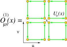
FIG. 1.: Graphical representation of the link products summed in creating ${\cal{O}}^{(1)}_{\mu\nu}(x)$.

$${\cal{O}}^{(1)}_{\mu\nu}(x) = U_{\mu}(x)\,U_{\nu}(x+\hat{\mu})\,U^{\dagger}_{\mu}(x+\hat{\nu})\,U^{\dagger}_{\nu}(x)$$ (15)

$$+ U_{\nu}(x)\,U^{\dagger}_{\mu}(x+\hat{\nu}-\hat{\mu})\,U^{\dagger}_{\nu}(x-\hat{\mu})\,U_{\mu}(x-\hat{\mu})$$ (16)

$$+ U^{\dagger}_{\mu}(x-\hat{\mu})\,U^{\dagger}_{\nu}(x-\hat{\mu}-\hat{\nu})\,U_{\mu}(x-\hat{\mu}-\hat{\nu})\,U_{\nu}(x-\hat{\nu})$$ (17)

$$+ U^{\dagger}_{\nu}(x-\hat{\nu})\,U_{\mu}(x-\hat{\nu})\,U_{\nu}(x+\hat{\mu}-\hat{\nu})\,U^{\dagger}_{\mu}(x)\,.$$ (18)

This well known definition for $F_{\mu\nu}(x)$ is commonly employed in the Clover term of the Sheikholeslami-Wohlert [27] improved quark action. Although, not everyone enforces the traceless nature of the Gell-Man matrices by subtracting off the trace as in Eq. (14).

Unfortunately, this definition has large ${\cal O}(a^{2})$ errors. These errors are most apparent in the topological charge. Even after hundreds of sweeps of cooling this simple definition fails to take on integer values. Errors are typically at the 10% level.

To improve the topological charge operator, we improve the definition of the field strength tensor $F_{\mu\nu}$ by removing ${\cal O}(a^{2})$ errors with a linear combination of plaquette and rectangle Wilson loops

$${\cal{O}}^{(2)}_{\mu\nu}(x)=c_{1}{\cal{O}}^{(1)}_{\mu\nu}(x)+\frac{c_{2}}{u_{0}^{2}}{\cal{I}}^{(2)}_{\mu\nu}(x)\,,$$ (19)

where the tadpole coefficient $u_{0}$ is defined in Eq. (5). Here ${\cal{I}}^{(2)}_{\mu\nu}(x)$ is the link products of $1\times 2$ and $2\times 1$ rectangles in the $\mu$-$\nu$ plane

$${\cal{I}}^{(2)}_{\mu\nu}(x) = U_{\mu}(x)U_{\mu}(x+\hat{\mu})U_{\nu}(x+2\hat{\mu})U^{\dagger}_{\mu}(x+\hat{\mu}+\hat{\nu})U^{\dagger}_{\mu}(x+\hat{\nu})U^{\dagger}_{\nu}(x)$$ (20)

$$+ U_{\mu}(x)U_{\nu}(x+\hat{\mu})U_{\nu}(x+\hat{\mu}+\hat{\nu})U^{\dagger}_{\mu}(x+2\hat{\nu})U^{\dagger}_{\nu}(x+\hat{\nu})U^{\dagger}_{\nu}(x)$$ (21)

$$+ U_{\nu}(x)U_{\nu}(x+\hat{\nu})U^{\dagger}_{\mu}(x-\hat{\mu}+2\hat{\nu})U^{\dagger}_{\nu}(x-\hat{\mu}+\hat{\nu})U^{\dagger}_{\nu}(x-\hat{\mu})U_{\mu}(x-\hat{\mu})$$ (22)

$$+ U_{\nu}(x)U^{\dagger}_{\mu}(x-\hat{\mu}+\hat{\nu})U^{\dagger}_{\mu}(x-2\hat{\mu}+\hat{\nu})U^{\dagger}_{\nu}(x-2\hat{\mu})U_{\mu}(x-2\hat{\mu})U_{\mu}(x-\hat{\mu})$$ (23)

$$+ U^{\dagger}_{\mu}(x-\hat{\mu})U^{\dagger}_{\mu}(x-2\hat{\mu})U^{\dagger}_{\nu}(x-2\hat{\mu}-\hat{\nu})U_{\mu}(x-2\hat{\mu}-\hat{\nu})U_{\mu}(x-\hat{\mu}-\hat{\nu})U_{\nu}(x-\hat{\nu})$$ (24)

$$+ U^{\dagger}_{\mu}(x-\hat{\mu})U^{\dagger}_{\nu}(x-\hat{\mu}-\hat{\nu})U^{\dagger}_{\nu}(x-\hat{\mu}-2\hat{\nu})U_{\mu}(x-\hat{\mu}-2\hat{\nu})U_{\nu}(x-2\hat{\nu})U_{\nu}(x-\hat{\nu})$$ (25)

$$+ U^{\dagger}_{\nu}(x-\hat{\nu})U_{\mu}(x-\hat{\nu})U_{\mu}(x+\hat{\mu}-\hat{\nu})U_{\nu}(x+2\hat{\mu}-\hat{\nu})U^{\dagger}_{\mu}(x+\hat{\mu})U^{\dagger}_{\mu}(x)$$ (26)

$$+ U^{\dagger}_{\nu}(x-\hat{\nu})U^{\dagger}_{\nu}(x-2\hat{\nu})U_{\mu}(x-2\hat{\nu})U_{\nu}(x+\hat{\mu}-2\hat{\nu})U_{\nu}(x+\hat{\mu}-\hat{\nu})U^{\dagger}_{\mu}(x)\,,$$ (27)

depicted in Fig. 2.

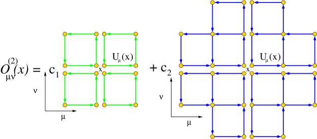
FIG. 2.: Graphical representation of the link products summed in creating ${\cal{O}}^{(2)}_{\mu\nu}(x)$.

The coefficients $c_{1}$ and $c_{2}$ are determined by combining Eqs. (11), (12) and (13) to remove ${\cal O}(a^{2})$ errors.

$$a^{2}\,F_{\mu\nu}(x_{0})=\frac{5}{3}\left[{\oint_{1\times{1}}A(x)\cdot{dx}}\right]-\frac{1}{6}\left[{\oint_{2\times{1}}A(x)\cdot{dx}}+{\oint_{1\times{2}}A(x)\cdot{dx}}\right]\,,$$ (28)

indicating the coefficients for the ${\cal O}(a^{2})$-improved $F_{\mu\nu}$ of Eq. (19) are

$$c_{1}=\frac{5}{3} \hskip 15.6491pt\rm{and}\hskip 15.6491pt c_{2}=-\frac{1}{6}.$$ (29)

IV Cooling and Smearing Algorithms

In this section we motivate and introduce an improved version of APE smearing. The motivation is based on improved cooling, and therefore we begin with a very brief overview of cooling algorithms. Cooling consists of minimizing the local action effectively one link at the time. The local action is that contribution to the action associated with a single link.

A Improved Cooling

Standard cooling minimizes the local Wilson action associated with a link at each link update. The local action associated with the link $U_{\mu}(x)$ is proportional to

$$S_{l}(x,\mu)=\sum_{\scriptstyle\nu\atop\scriptstyle\nu\neq\mu}{{\rm{Re\,Tr}}}\left(1-U_{\mu}(x)\Sigma_{\mu\nu}(x)\right)\,,$$ (30)

where $\Sigma_{\mu\nu}(x)$ is the sum of the two staples associated with $U_{\mu}(x)$ lying in the $\mu$-$\nu$ plane

$$\Sigma_{\mu\nu}(x)=U_{\nu}(x+\hat{\mu})U^{\dagger}_{\mu}(x+\hat{\nu})U^{\dagger}_{\nu}(x)+U^{\dagger}_{\nu}(x+\hat{\mu}-\hat{\nu})U^{\dagger}_{\mu}(x-\hat{\nu})U_{\nu}(x-\hat{\nu})\,.$$ (31)

The local action associated with the link $U_{\mu}(x)$ is minimized in standard cooling by a minimization process, i.e., by replacing the original link by the link $U_{\mu}(x)$ which optimizes

$${\rm{max}}\,{{\rm{Re\,Tr}}}\left(U_{\mu}(x)\sum_{\scriptstyle\nu\atop\scriptstyle\nu\neq\mu}\Sigma_{\mu\nu}(x)\right)\,.$$ (32)

Improved cooling proceeds in exactly the same manner, but with the plaquette-based staples replaced with the linear combination of plaquette-based staples and rectangle-based staples. For improved cooling we use

$${\rm{max}}\,{{\rm{Re\,Tr}}}\left(U_{\mu}(x)\sum_{\scriptstyle\nu\atop\scriptstyle\nu\neq\mu}\Sigma^{I}_{\mu\nu}(x),\right)\,.$$ (33)

Where

$$\Sigma^{I}_{\mu\nu}={5\over 3}\,\Sigma_{\mu\nu}+{1\over 12\,u_{o}^{2}}\,\Sigma^{R}_{\mu\nu}\,,$$ (34)

and

$$\Sigma^{R}_{\mu\nu}(x) = U_{\nu}(x+\hat{\mu})U_{\nu}(x+\hat{\nu}+\hat{\mu})U^{\dagger}_{\mu}(x+2\hat{\nu})U^{\dagger}_{\nu}(x+\hat{\nu})U^{\dagger}_{\nu}(x)$$ (35)

$$+ U_{\mu}(x+\hat{\mu})U_{\nu}(x+2\hat{\mu})U^{\dagger}_{\mu}(x+\hat{\mu}+\hat{\nu})U^{\dagger}_{\mu}(x+\hat{\nu})U^{\dagger}_{\nu}(x)$$ (36)

$$+ U_{\nu}(x+\hat{\mu})U^{\dagger}_{\mu}(x+\hat{\nu})U^{\dagger}_{\mu}(x+\hat{\nu}-\hat{\mu})U^{\dagger}_{\nu}(x-\hat{\mu})U_{\mu}(x-\hat{\mu})$$ (37)

$$+ U^{\dagger}_{\nu}(x+\hat{\mu}-\hat{\nu})U^{\dagger}_{\nu}(x+\hat{\mu}-2\hat{\nu})U^{\dagger}_{\mu}(x-2\hat{\nu})U_{\nu}(x-2\hat{\nu})U_{\nu}(x-\hat{\nu})$$ (38)

$$+ U_{\mu}(x+\hat{\mu})U^{\dagger}_{\nu}(x+2\hat{\mu}-\hat{\nu})U^{\dagger}_{\mu}(x+\hat{\mu}-\hat{\nu})U^{\dagger}_{\mu}(x-\hat{\nu})U_{\nu}(x-\hat{\nu})$$ (39)

$$+ U^{\dagger}_{\nu}(x+\hat{\mu}-\hat{\nu})U^{\dagger}_{\mu}(x-\hat{\nu})U^{\dagger}_{\mu}(x-\hat{\nu}-\hat{\mu})U_{\nu}(x-\hat{\nu}-\hat{\mu})U_{\mu}(x-\hat{\mu})\,.$$ (40)

The mean-field factor $u_{0}$ is updated following each sweep through the lattice and rapidly goes to 1 as perturbative tadpole contributions are removed. As we wish to study ${\cal O}(a^{2})$–improved cooling, the coefficients are based on those of the action [17, 28]. While this action improves contact with QCD, this choice of action does not completely stabilize instantons on the lattice [15, 29]. Removal of ${\cal O}(a^{2})$ errors and stabilization of instantons requires the consideration of additional loops [16, 30]. The preferred algorithm for finding the $U_{\mu}(x)$ which maximizes Eq. (32) is based on the Cabbibo-Marinari [25] pseudo-heat-bath algorithm for constructing $SU(3)$ -color gauge configurations. There, operations are performed at the SU(2) level where the algorithm is transparent.

An element of $SU(2)$  may be parameterized as, $U=a_{0}I+i\,\vec{a}\cdot\vec{\sigma}$, where $a$ is real and $a^{2}=1$. Since sums of products of SU(2) matrices are proportional to SU(2) matrices,

$$\sum_{\scriptstyle\nu\atop\scriptstyle\nu\neq\mu}\Sigma^{I}_{\mu\nu}(x)=k\overline{U}_{\mu}(x)\,,$$ (41)

where $\overline{U}_{\mu}(x)\in\mbox{$SU(2)$}$ and

$$k^{2}\equiv{\det\left(\sum_{\scriptstyle\nu\atop\scriptstyle\nu\neq\mu}\Sigma^{I}_{\mu\nu}(x)\right)}\,.$$ (42)

The maximum of the expression

$${{\rm{Re\,Tr}}}\left(U_{\mu}(x)\sum_{\scriptstyle\nu\atop\scriptstyle\nu\neq\mu}\Sigma^{I}_{\mu\nu}(x)\right)={{\rm{Re\,Tr}}}\left(k\,U_{\mu}(x)\,\overline{U}_{\mu}(x)\right)\,,$$ (43)

is achieved when

$${{\rm{Re\,Tr}}}\left(U_{\mu}(x)\overline{U}_{\mu}(x)\right)={{\rm{Re\,Tr}}}(I)\,,$$ (44)

which requires the link to be updated as

$$U_{\mu}(x){\to}U^{\prime}_{\mu}(x)=\overline{U}^{-1}_{\mu}(x)=\overline{U}^{\dagger}_{\mu}(x)=\left(\sum_{\scriptstyle\nu\atop\scriptstyle\nu\neq\mu}{\Sigma^{I}_{\mu\nu}(x)\over k}\right)^{\dagger}\,.$$ (45)

At the $SU(3)$ level, we successively apply this algorithm to the three diagonal $SU(2)$ subgroups of $SU(3)$ [25].

When considering an improved cooling algorithm it is crucial to loop over sufficient SU(2) subgroups to ensure that the subtle effects of the higher dimension operators introduced in improving the action are reflected in the final SU(3) link. It is easy to imagine that only two or three SU(2) subgroups may not take the SU(3) link close enough to the optimal link for the effects of improvement to be properly seen. We find consideration of the three diagonal $SU(2)$ subgroups looped over twice to be optimal. In fact we have seen round off errors actually increase the action if too many loops are made.

The $u_{0}$ factor of Eq. (34) is not held fixed during the improved cooling iteration. Starting from the value determined during the thermalization process, $u_{0}$ is updated after every sweep through the lattice. After a few sweeps of improved cooling the value quickly converges to 1 which is a good indication that short distance tadpole effects are being removed in the smoothing procedure.

Finally it must be understood that cooling proceeds effectively one link at a time. That is, links involved in constructing $\Sigma^{I}_{\mu\nu}(x)$ are not updated simultaneously with $U_{\mu}(x)$. In fact it is a nontrivial task identifying which links can be simultaneously updated on a massively parallel computer [26].

B Improved Smearing

In this section we consider the APE smearing [1] algorithm. We extend this algorithm to produce an improved version, motivated by the success of the improved cooling program.

1 Reunitarization of the Links

APE smearing is a gauge equivariant [32] prescription for smearing a link $U_{\mu}(x)$ with its nearest neighbors $U_{\mu}(x+\hat{\nu})$, where $\hat{\nu}$ is transverse to $\hat{\mu}$. The APE smearing process takes the form

$$U_{\mu}(x)\longrightarrow{U_{\mu}^{\prime}(x)} = (1-\alpha)U_{\mu}(x)+\frac{\alpha}{6}\sum_{\scriptstyle\nu\atop\scriptstyle\nu\neq\mu}\Sigma_{\mu\nu}^{\dagger}(x)\,,$$ (46)

$$U_{\mu}(x) = {\cal P}{U_{\mu}^{\prime}(x)}\,,$$ (47)

where $\Sigma_{\mu\nu}(x)$ is the sum of the two staples associated with $U_{\mu}(x)$ defined in Eq. (31) and ${\cal P}$ is a projection operator which projects the smeared link back onto $SU(3)$.

The reunitarization procedure is of central importance when smearing is applied to the gauge links because the APE smearing operation produces links outside the $SU(3)$ gauge group in the intermediate stage of smearing. The link between smearing and cooling is established via the manner in which smeared links are projected back onto SU(3). The preferred approach is to select the link variable $U_{\mu}(x)$ that maximizes the quantity

$${{\rm{Re\,Tr}}}\left(U_{\mu}(x)U_{\mu}^{\prime\dagger}(x)\right)\,.$$ (48)

In this case a clear connection to cooling is established when $\alpha\to 1$ as

$$\max{{\rm{Re\,Tr}}}\left(U_{\mu}(x)U_{\mu}^{\prime\dagger}(x)\right)=\max{{\rm{Re\,Tr}}}\left(U_{\mu}(x)\sum_{\scriptstyle\nu\atop\scriptstyle\nu\neq\mu}\Sigma_{\mu\nu}(x)\right)\,,$$ (49)

which is precisely the condition of Eq. (32) for cooling. In other words, projection of the smeared link back onto the gauge group via Eq. (49) selects the link which minimizes the local action. Improvement of the staple based on the action will aid in removing ${\cal O}(a^{2})$ errors encountered in the $SU(3)$ projection. In practice, the same Cabibbo-Marinari-based cooling method of operating on $SU(2)$ subgroups may be used to obtain the ultimate SU(3) link.

However there is one very important difference remaining between APE smearing and cooling. While cooling effectively updates one link at a time, feeding the smoothed link immediately into the next link update, APE smearing proceeds uniformly with all links being simultaneously updated. Smoothed links are not introduced into the algorithm until the next iteration of the APE smearing process takes place.

It is this latter point that provides the form factor interpretation of APE smearing in fat-link fermion actions [4]. There smearing can be understood to introduce a form factor suppressing the coupling of gluons to quarks at the edge of the Brillouin zone where lattice artifacts are most problematic. The form factor analysis restricts the smearing fraction to the range $0\leq\alpha\leq 3/4$. Indeed in practice, smearing fractions beyond 3/4 do not lead to smooth gauge configurations.

2 Improving Smearing

Having made firm contact with cooling it is clear that replacing the simple staple of Eq. (31) with the improved staple of Eq. (34) may lead to a realization of the benefits of improved cooling within APE smearing. Hence we define improved smearing to be an APE smearing step in which

$$U_{\mu}(x)\longrightarrow{U_{\mu}^{\prime}(x)} = (1-\alpha)U_{\mu}(x)+\frac{\alpha}{6}\sum_{\scriptstyle\nu\atop\scriptstyle\nu\neq\mu}\Sigma_{\mu\nu}^{I\dagger(x)}\,,$$ (50)

$$U_{\mu}(x) = {\cal P}{U_{\mu}^{\prime}(x)}\,,$$ (51)

where $\Sigma_{\mu\nu}^{I}(x)$ is the improved staple of Eq. (34).

Signatures of improvement include the preservation of structures in the action density distribution under smearing. ${\cal O}(a^{2})$ errors in the standard Wilson action act to underestimate the local action and destroy topologically nontrivial field configurations [15]. Improved smearing will have reduced ${\cal O}(a^{2})$ errors and hence better preserve topologically nontrivial field configurations. Hence an associated signature of improvement is the stability of topological charge under hundreds of smearing sweeps. Of course, one could alter the coefficients of the improvement terms to stabilize instantons [15] at the expense of introducing ${\cal O}(a^{2})$ errors into the smoothing action.

The extended nature of the staple will alter the stability range of $\alpha$. Where standard APE smearing provides the range $0\leq\alpha\leq 3/4$, we find the upper stability limit lies below $\alpha=0.6$.

V Numerical Simulations

We analyze two sets of gauge field configurations generated using the Cabibbo-Marinari [25] pseudo-heat-bath algorithm with three diagonal $SU(2)$ subgroups looped over twice. Details may be found in Table I. As discussed in the introduction, analysis of a few configurations proves to be sufficient to resolve the nature of the algorithms under investigation. We consider eleven $16^{3}\times{32}$ configurations and six $24^{3}\times{36}$ configurations. For each configuration we separately perform 200 sweeps of cooling and 200 sweeps of improved cooling. We explore 200 sweeps of APE smearing at seven values of the smearing fraction and 200 sweeps of improved smearing at five values of the smearing fraction. For APE smearing we consider $\alpha=0.10$, 0.20, 0.30, 0.40, 0.50, 0.60, and 0.70. Similarly for improved smearing we consider $\alpha=0.10$ to 0.50 at intervals of 0.10. The extended nature of the staple alters the stability range of $\alpha$ to lie below $\alpha=0.6$.

For clarity, we define the number of times an algorithm is applied to the entire lattice as $n_{\rm{c}}$, $n_{\rm{Ic}}$, $n_{\rm{ape}}(\alpha)$ and $n_{\rm{Iape}}(\alpha)$ for cooling, improved cooling, APE smearing and improved smearing respectively. We monitor both the total action normalized to the single instanton action $S_{0}=8\pi^{2}/g^{2}$ and the topological charge operators, $Q_{\rm{L}}$ and $Q^{\rm{Imp}}_{\rm{L}}$, from which we observe their evolution as a function of the appropriate sweep variable and smearing fraction $\alpha$.

A The Influence Of The Number Of Subgroups On The Gauge Group.

In this section we describe the influence of including additional $SU(2)$ subgroups in constructing the gauge group $SU(3)$ and explore the impact it has on the smoothing procedure. The Cabibbo-Marinari algorithm [25] constructs the $SU(N)$ gauge groups using $SU(2)$ subgroups. It is understood that the minimal set required to construct $SU(3)$ matrices is two diagonal $SU(2)$ subgroups. After having performed cooling on gauge field configurations we noticed that the resulting cooled gauge field configurations were not smooth even after a large number of smoothing steps. Adding a third $SU(2)$ subgroup made a significant difference in the resulting smoothness.

We explored further by simply performing additional cycles, $n_{\rm{cycle}}$, around the three diagonal $SU(2)$  subgroups. We monitored the smoothing rate using both the Standard Wilson and the improved action according to the cycle number being set to $n_{\rm{cycle}}=1,2$ and 3. Based on the evolution of the action, we found that the optimum cooling rate on gauge field configurations is achieved using the three diagonal $SU(2)$  subgroups cycled over twice, $n_{\rm{cycle}}=2$. Cycling more than twice provides very little further reduction of the action and round off errors may actually increase the action on occasion. Hence two cycles over the three diagonal $SU(2)$ subgroups is sufficient to precisely create the $SU(3)$ link which minimizes the local action. This determination is crucial to ensuring the effects of our improved action are fully reflected in the $SU(3)$ link.

We also monitored the evolution of the topological charge with respect to the above number of cycles. On the $16^{3}\times{32}$ lattice with spacing of $a=0.165(2)$ fm, we observe a disagreement of the trajectories for the topological charge for different numbers of the $SU(2)$ subgroups cycles. Fig. 3 displays results for standard cooling and Fig. 4

FIG. 3.: The evolution of the topological charge estimated by the improved operator as a function of standard cooling sweeps $n_{\rm{c}}$ for various numbers of $SU(2)$ subgroups. The curves are for a typical configuration from the $16^{3}\times{32}$ lattices where $a=0.165(2)$ fm. The parameter cycle describes the number of times the three diagonal $SU(2)$ subgroups are cycled over.

FIG. 4.: The evolution of the topological charge estimated by the improved operator as a function of improved cooling sweeps $n_{\rm{Ic}}$ for various numbers of cycles over the three diagonal $SU(2)$ subgroups. The curves are for the same configuration illustrated in Fig.  3.

displays similar results for improved cooling. A comparison of Figs. 3 and 4 indicates the trajectories also differ between cooling and improved cooling.

Hence we see subtle differences in the algorithms leading to dramatic differences in the topological charge. One must conclude that a lattice spacing of 0.165(2) fm is too coarse for a serious study of topology in $SU(3)$ gauge fields using the algorithms considered here. The difficulty lies in the fact that the algorithms have a dislocation threshold typically a little over two lattice spacings [16, 21]. Instantons with a size smaller than the dislocation threshold are removed during the process of smoothing. While this threshold has the desireable property of removing lattice artifacts, we note that twice the lattice spacing is 0.33 fm. Minor differences in the dislocation thresholds of the various algorithms will cause some (anti)instantons to survive under one algorithm where they are removed under another.

On the other hand, a lattice spacing the order of 0.077(1) fm appears to allow a meaningful study of topology in $SU(3)$ gauge theory. Twice this lattice spacing is 0.15 fm, well below the typical size of instantons [24].

We also note here the accuracy with which our improved topological charge operator reproduces integer values. These results should be contrasted with the usual 10% errors of the unimproved operator at similar lattice spacings. Such errors on a topological charge of 5 can lead to the uncomfortable result of $Q\simeq 4.5$ when the unimproved operator is used.

With the finer $24^{3}\times{36}$ lattice at $\beta=5.00$, we observe perfect agreement among trajectories for different numbers of cycles of the three $SU(2)$ subgroups. Moreover, the topological charge remains stable for hundreds of sweeps following the first three sweeps. Figures 5 and 6 compare the topological charge evolution for cooling versus improved cooling for six configurations. In every case, the two algorithms produce the same topological charge for a given configuration.

FIG. 5.: The evolution curve for the topological charge estimated via the improved operator as a function of cooling sweeps $n_{\rm{c}}$ for six configurations on the $24^{3}\times{36}$ lattices at $\beta=5.00$ where $a={0.077(1)}$ fm.

FIG. 6.: The evolution curve for the topological charge estimated via the improved operator as a function of improved cooling sweeps $n_{\rm{Ic}}$ for the same six configurations from the $24^{3}\times{36}$ lattices at $\beta=5.00$ illustrated in Fig. 5.

B The Action

We begin by considering the action evolution on both lattices. Here we report the action divided by the single instanton action $\mbox{$S_{0}$}=8\pi^{2}/g^{2}$. It is important to note that although the $24^{3}\times{36}$ lattice has almost four times more lattice sites than the $16^{3}\times{32}$ lattice, the physical volume is smaller by almost a factor of three. As such the typical topological charges encountered are smaller in magnitude.

Figs. 7, 8, 9, and 10 report the typical evolution of the action under standard cooling, improved cooling, APE smearing and improved smearing respectively. Inspection of the figures reveals that improved cooling preserves the action better than standard cooling over a couple hundred sweeps. As expected, standard APE smearing remains slower than cooling or improved cooling even at our most efficient smearing fraction ($\alpha=0.70$). Similar results are observed for improved smearing at our most efficient smearing fraction of $\alpha=0.50$ in Fig. 10.

FIG. 7.: The ratio $S/S_{0}$ as a function of standard cooling sweeps $n_{\rm{c}}$ for five configurations on the $24^{3}\times{36}$ lattice at $\beta=5.0$. The single instanton action is $S_{0}=8\pi^{2}/g^{2}$.

FIG. 8.: The ratio $S/S_{0}$ as a function of improved cooling sweeps $n_{\rm{Ic}}$ for five configurations on the $24^{3}\times{36}$ lattice at $\beta=5.0$. The rate of cooling is seen to be somewhat slower than that for the standard cooling.

FIG. 9.: The ratio $S/S_{0}$ as a function of APE smearing sweeps $n_{\rm{ape}}(\alpha)$ for one configuration on the $24^{3}\times{36}$ lattice at $\beta=5.0$. Each curve has an associated smearing fraction $\alpha$. The rate of lowering the action for the maximum stable smearing fraction ($\approx{0.75}$) is seen to be less than that for the other standard or improved cooling.

FIG. 10.: The ratio $S/S_{0}$ as a function of improved smearing sweeps $n_{\rm{Iape}}(\alpha)$ for one configuration on the $24^{3}\times{36}$ lattice at $\beta=5.0$. Each curve has an associated smearing fraction $\alpha$. We see that this is the slowest of the four algorithms for lowering the action as a function of the sweep number.

Based on these observations, one concludes that the fastest way to remove the short range quantum fluctuations on an ${\cal O}(a^{2})$ gauge field configuration, is through standard cooling, which lowers the action more rapidly than improved cooling as a function of cooling sweep. In turn we see that improved cooling is faster than the maximum stable standard APE smearing, which is faster than the maximum stable improved smearing. This is illustrated by Figs. 7–10. It is important to emphasize that the fastest way of removing these fluctuations is not necessarily the best as far as the topology is concerned. It is already established that the ${\cal O}(a^{2})$ errors of the standard Wilson action act to underestimate the action [15]. These errors spoil instantons which might otherwise survive under improved cooling.

C Topological Charge from Cooling and Smearing

We begin by considering the $16^{3}\times{32}$ lattices having a lattice spacing of $a=0.165(2)$ fm. In Fig. 11, we plot the evolution curve for the improved topological charge as a function of the cooling sweep number, $n_{\rm{c}}$, for six of our configurations. Similarly in Fig. 12, for the same six configurations we plot the improved topological charge operator but this time as a function of improved cooling sweep $n_{\rm{Ic}}$. The line types in Figs. 11 and 12 correspond to the same underlying configurations and are to be directly compared. For example, the solid curve corresponds to the same gauge field configuration in both figures but with a different algorithm applied to it. From these two figures we notice the two cooling methods lead to completely different values for the topological charge.

FIG. 11.: $Q^{\rm{Imp}}_{\rm{L}}$ versus $n_{\rm{c}}$ for six configurations on the $16^{3}\times{32}$ lattices at $\beta=4.38$, $a=0.165(2)$ fm. Each line corresponds to a different configuration.

FIG. 12.: $Q^{\rm{Imp}}_{\rm{L}}$ versus $n_{\rm{Ic}}$ for six configurations on the $16^{3}\times{32}$ lattices. The different line types identifying different configurations match the configurations identified in Fig. 11.

Improved cooling brings stability to the evolution of the topological charge whereas standard cooling gives rise to numerous fluctuations to the topological charge. For improved cooling, plateaus appear after about forty sweeps and persist for hundreds of sweeps. This is a celebrated feature of improved cooling.

This algorithmic sensitivity of the topological charge is also seen in Figs. 13 and 14, for APE and improved smearing on a single configuration (the solid line of Figs. 11 and 12). Within APE smearing or improved smearing, the topological charge trajectories follow similar patterns but different rates for various smearing fractions. However, APE smearing leads to values for the topological charge which are different from that obtained under improved smearing. An important point is that improved smearing stabilizes the topological charge at 95 sweeps for $\alpha=0.5$, whereas standard smearing shows no sign of stability until 140 iterations at $\alpha=0.5$. Hence we see significant improvement in the topological aspects of the gauge field configurations under improved smearing.

FIG. 13.: The evolution of $Q^{\rm{Imp}}_{\rm{L}}$ using APE smearing as a function of APE smearing sweep $n_{\rm{ape}}(\alpha)$ on the $16^{3}\times{32}$ lattice at $\beta=4.38$. Here different line types correspond to different smearing fractions.

FIG. 14.: The evolution of $Q^{\rm{Imp}}_{\rm{L}}$ using improved smearing as a function of APE smearing sweep $n_{\rm{Iape}}(\alpha)$ on the $16^{3}\times{32}$ lattice at $\beta=4.38$. Here different line types correspond to different smearing fractions.

On our finer lattice, we find a completely different behavior for the topological charge evolution. The topological charge is established very quickly; after a few sweeps in the case of cooling or improved cooling as illustrated in Figs. 5 and 6. The topological charge persists without fluctuation for hundreds of sweeps, both for cooling and for smearing as illustrated in Figs. 15 and 16 for APE and improved smearing respectively. Moreover, the topological charge is independent of the smearing algorithm.

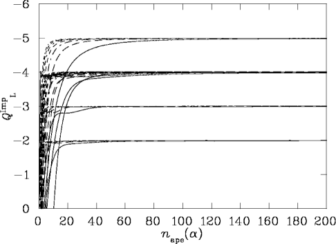
FIG. 15.: The evolution of $Q^{\rm{Imp}}_{\rm{L}}$ using APE smearing as a function of APE smearing sweep $n_{\rm{ape}}(\alpha)$ on the $24^{3}\times{36}$ lattice at $\beta=5.00$. Here different line types correspond to different smearing fractions.

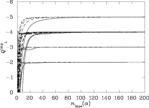
FIG. 16.: The evolution of $Q^{\rm{Imp}}_{\rm{L}}$ using APE smearing as a function of APE smearing sweep $n_{\rm{Iape}}(\alpha)$ on the $24^{3}\times{36}$ lattice at $\beta=5.00$. Here different line types correspond to different smearing fractions.

These results are to be compared with Fig. 11 and Fig. 12, where transitions are observed even with improved cooling on the coarser lattice with $a=0.165(2)$ fm. The results on our fine lattice suggest the characteristic size of instantons is much larger than the dislocation threshold, such that the topological structure of the gauge fields is smooth at the scale of the threshold.

In Fig. 15 for standard APE smearing we observe a slower convergence to integer topological charge than in Fig. 16 for improved smearing when ${0.1}\leq\alpha\leq{0.5}$. This feature of improved smearing is illustrated in detail in Fig. 17. However, APE smearing has the advantage to allow values for the smearing fraction up to $\alpha=0.70$ which cannot be accessed by improved smearing.

FIG. 17.: The evolution of the improved topological charge, $Q^{\rm{Imp}}_{\rm{L}}$, as a function of standard APE smearing sweeps, $n_{\rm{ape}}(\alpha)$, for ${0.1}\leq\alpha\leq{0.7}$ (solid lines) is compared to improved smearing sweeps, $n_{\rm{Iape}}(\alpha)$, (dotted-dashed lines) for the same smearing fractions ${0.1}\leq\alpha\leq{0.5}$ on the $24^{3}\times{36}$ lattice at $\beta=5.00$. The horizontal dotted-dashed line is $Q^{\rm{Imp}}_{\rm{L}}=-4$.

Having demonstrated that it is possible to precisely match the behavior of the algorithms on fine lattice spacings, we proceed to calibrate the efficiency of these algorithms in the following section.

VI Smoothing Algorithm Calibration

Here we calibrate the relative rate at which quantum fluctuations are removed from typical field configurations by the various algorithms. The calibration is done using the action normalized to the single instanton action, $S/S_{0}$, on both, the $16^{3}\times{32}$ lattices and $24^{3}\times{36}$ lattices. The action normalized to the single instantons action, $S/S_{0}$, is of particular interest because it provides insight into the lattice content as well as the rate at which the quantum fluctuations are removed.

While there is no doubt that the algorithms may be accurately calibrated on the fine $24^{3}\times{36}$ lattice, the $16^{3}\times{32}$ lattice with $a=0.165(2)$ fm presents more of a challenge. As a result, in most cases we will show the graphs produced from the $16^{3}\times{32}$ lattice analysis and simply present the numerical results for both the $16^{3}\times{32}$ and $24^{3}\times{36}$ lattices.

The numerical results are summarized in Tables II, III, and VI for the $16^{3}\times{32}$ lattices and in Tables IV, V, and VII for the $24^{3}\times{36}$ lattices.

A APE Smearing and Improved Smearing Calibration.

To calibrate the rate at which the algorithm reduces the action we record the nearest number of sweeps required to reach a given threshold in $S/S_{0}$. The action thresholds are spaced logarithmically to obtain a uniform distribution in the number of sweeps required to reach a threshold. The relative rates of smoothing are established by comparing the relative number of sweeps required to reach a particular threshold.

Here we calibrate the APE smearing algorithm characterized by the smearing fraction $\alpha$ and the number of smearing iterations $n_{\rm{ape}}(\alpha)$. The different threshold crossings are characterized by the number of sweeps required to reach that threshold, $n_{\rm{ape}}(\alpha)$. In Fig. 18 we show the number of sweeps required to reach a threshold when $\alpha=0.5$, $n_{\rm{ape}}(0.50)$, relative to that required for other $\alpha$ values, $n_{\rm{ape}}(\alpha)$. We plot these relative smoothing rates as a function of $n_{\rm{ape}}(\alpha)$ such that low $S/S_{0}$ thresholds are reached after hundreds of iterations of the smoothing algorithm. Fig. 19 shows similar results for improved smearing. In these figures and in the following analysis, we omit thresholds that result in fewer than five smoothing iterations as these points produce integer discretization errors of more than 20%.

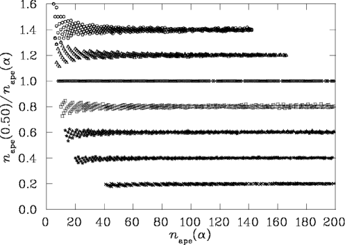
FIG. 18.: The ratio $n_{\rm{ape}}(0.50)/\mbox{$n_{\rm{ape}}(\alpha)$}$ versus $n_{\rm{ape}}(\alpha)$ for numerous $S/S_{0}$ thresholds on the $16^{3}\times{32}$ lattice at $\beta=4.38$. From top to bottom the data point bands correspond to $\alpha=0.7$, 0.6, 0.5, 0.4, 0.3, 0.2, and 0.1.

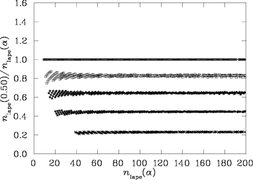
FIG. 19.: The ratio $n_{\rm{Iape}}(0.50)/\mbox{$n_{\rm{Iape}}(\alpha)$}$ versus $n_{\rm{Iape}}(\alpha)$ for numerous $S/S_{0}$ thresholds on the $16^{3}\times{32}$ lattice at $\beta=4.38$. From top to bottom the data point bands correspond to $\alpha=0.5$, 0.4, 0.3, 0.2, and 0.1.

Both standard and improved smearing algorithms have a relative smoothing rate which is independent of the amount of smoothing done. By calculating the average value for each of the bands in Figs. 18 and 19, we can investigate the dependence of the average relative smoothing rate $\langle n_{\rm{ape}}(0.50)/\mbox{$n_{\rm{ape}}(\alpha)$}\rangle$ on $\alpha$.

Fig. 20 illustrates a linear fit to the data constrained to pass through the origin. We find $\langle n_{\rm{ape}}(0.50)/\mbox{$n_{\rm{ape}}(\alpha)$}\rangle=2.00\,\alpha$ such that

$$\frac{n_{\rm{ape}}(\alpha^{\prime})}{\mbox{$n_{\rm{ape}}(\alpha)$}}=\frac{\alpha}{\alpha^{\prime}}$$ (52)

in agreement with our earlier analysis [22]. The extent to which this relationship holds can be verified [22] by plotting the ratio $\alpha^{\prime}n_{\rm{ape}}(\alpha^{\prime})/\alpha\mbox{$n_{\rm{ape}}(\alpha)$}$ and comparing the results to 1.

FIG. 20.: Illustration of the dependence of $\langle n_{\rm{ape}}(0.50)/\mbox{$n_{\rm{ape}}(\alpha)$}\rangle$ for APE smearing on the smearing fraction $\alpha$. The solid line is a linear fit to the data constrained to pass through the origin.

In plotting the band averages for the improved smearing algorithm of Fig. 19 in Fig. 21, one finds a small deviation of the points from the line $y=2\,\alpha$. This suggests that Eq. (52) is not sufficiently general for the improved smearing case.

FIG. 21.: Illustration of the dependence of $<n_{\rm{Iape}}(0.50)/\mbox{$n_{\rm{Iape}}(\alpha)$}>$ for APE smearing on the improved smearing fraction $\alpha$. The solid line fit is constrained to pass through the origin.

A better approximation to establish the $\alpha$ dependence, that is similar to Eq. (52) and contains Eq. (52) is

$$\frac{n_{\rm{Iape}}(\alpha^{\prime})}{\mbox{$n_{\rm{Iape}}(\alpha)$}}=\left(\frac{\alpha}{\alpha^{\prime}}\right)^{\delta}\,,$$ (53)

where $\delta$ is equal to one in the case of standard APE smearing and can deviate away from one for improved smearing.

In Fig. 22, the logarithm of Eq. (53) is plotted. The slope of the data provides $\delta=0.914(1)$ for both the $16^{3}\times{32}$ and the $24^{3}\times{36}$ lattices. We also verified $\delta=1.00$ for the APE smearing data. Fig. 23 plots the ratio of the left- and right-hand sides of Eq. (53) as a function of $n_{\rm{Iape}}(\alpha)$ for $\alpha^{\prime}>\alpha$. The ratio is one as expected with 5% for large amounts of smearing where integer discretization errors are minimized. Throughout the following analysis, $\delta$ is fixed at 0.914(1).

FIG. 22.: Illustration of the dependence of $\ln\left(<n_{\rm{Iape}}(0.50)/\mbox{$n_{\rm{Iape}}(\alpha)$}>\right)$ on the improved smearing fraction $\alpha$ for improved smearing. The solid line fit indicates $\delta=0.914$.

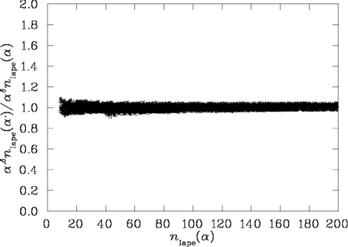
FIG. 23.: Illustration of the degree to which the relation Eq. (53) is satisfied for improved smearing. Here the entire data set is plotted for $\alpha$ and $\alpha^{\prime}=0.5$, 0.4, 0.3, 0.2 and 0.1. Data are from $16^{3}\times{32}$ lattice at $\beta=4.38$.

B APE and Improved smearing cross calibration.

In this section we focus on the cross calibration of the smearing algorithms. In Fig. 24, we compare the number of improved smearing sweeps required to reach a threshold for various improved smearing fractions relative to APE smearing at $\alpha=0.5$. The lowest band corresponds to an improved smearing fraction of 0.10. From this, we conclude that for low $\alpha$ values APE smearing and improved smearing produce roughly equivalent smeared configurations. However, there are some evident differences in the rate at which both algorithms perform. For intermediate to large $\alpha$ there is curvature in the bands. Early in the smearing process, fewer sweeps of improved smearing are required to reach a threshold. That is, improved smearing removes action faster than APE smearing in the early stages of smearing. This behavior is also manifest in the analogous results for the fine $24^{3}\times{36}$ lattice. As emphasized in the discussion surrounding Fig. 17, improved smearing also provides a topological charge closer to an integer than APE smearing. Together, these two properties of improved smearing identify a genuine improvement in the smearing process.

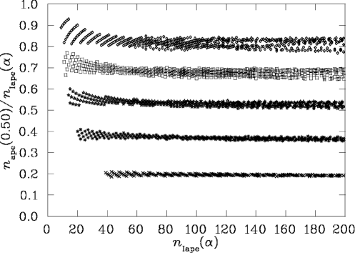
FIG. 24.: The ratio $n_{\rm{ape}}(0.50)/\mbox{$n_{\rm{Iape}}(\alpha)$}$ versus $n_{\rm{Iape}}(\alpha)$ for numerous threshold actions on the $16^{3}\times{32}$ lattice at $\beta=4.38$. From top to bottom the data point bands correspond to improved smearing fractions $\alpha=0.5$, 0.4, 0.3, 0.2, and 0.1.

For the coarse $16^{3}\times{32}$ lattice data, the bands are thick for large smearing fractions indicating improved smearing does perform significantly different from standard APE smearing. Contributions from individual configurations are clearly visible as lines within the bands. This structure is due to the coarse lattice spacing of 0.165(2) fm which reveals differences between the algorithms. Such structure is not seen in the fine $24^{3}\times{36}$ lattice results. There a precise calibration is possible.

In Tables II and III, we report the averages of each band for APE and improved smearing on the $16^{3}\times{32}$ lattices. In Tables IV and V we report similar results for the $24^{3}\times{36}$ lattices.

TABLE II.: The averages of the ratios $<n_{\rm{ape}}(0.50)/\mbox{$n_{\rm{ape}}(\alpha)$}>$ and $<n_{\rm{Iape}}(0.50)/\mbox{$n_{\rm{ape}}(\alpha)$}>$ for various smearing fractions $\alpha$ from the $16^{3}\times{32}$ lattice at $\beta=4.38$.

	$\alpha$ for APE smearing
	0.10	0.20	0.30	0.40	0.50	0.60	0.70
$n_{\rm{ape}}(0.50)$	0.195(1)	0.394(2)	0.595(3)	0.797(4)	1.0	1.203(1)	1.407(1)
$n_{\rm{Iape}}(0.50)$	0.227(1)	0.465(1)	0.706(1)	0.948(1)	1.189(1)	1.431(1)	1.673(1)

TABLE III.: The averages of the ratios $<n_{\rm{ape}}(0.50)/\mbox{$n_{\rm{Iape}}(\alpha)$}>$ and $<n_{\rm{Iape}}(0.50)/\mbox{$n_{\rm{Iape}}(\alpha)$}>$ for various smearing fractions $\alpha$ from the $16^{3}\times{32}$ lattice at $\beta=4.38$.

	$\alpha$ for improved smearing
	0.10	0.20	0.30	0.40	0.50
$n_{\rm{ape}}(0.50)$	0.196(1)	0.376(3)	0.543(1)	0.697(1)	0.842(1)
$n_{\rm{Iape}}(0.50)$	0.228(1)	0.442(1)	0.641(1)	0.827(1)	1.0

TABLE IV.: The averages of the ratios $<n_{\rm{ape}}(0.50)/\mbox{$n_{\rm{ape}}(\alpha)$}>$ and $<n_{\rm{Iape}}(0.50)/\mbox{$n_{\rm{ape}}(\alpha)$}>$ for various smearing fractions $\alpha$ from the $24^{3}\times{36}$ lattice at $\beta=5.00$.

	$\alpha$ for APE smearing
	0.10	0.20	0.30	0.40	0.50	0.60	0.70
$n_{\rm{ape}}(0.50)$	0.195(1)	0.395(1)	0.595(1)	0.797(1)	1.0	1.205(1)	1.410(1)
$n_{\rm{Iape}}(0.50)$	0.227(1)	0.462(1)	0.698(1)	0.937(1)	1.176(1)	1.416(1)	1.658(1)

TABLE V.: The averages of the ratios $<n_{\rm{ape}}(0.50)/\mbox{$n_{\rm{Iape}}(\alpha)$}>$ and $<n_{\rm{Iape}}(0.50)/\mbox{$n_{\rm{Iape}}(\alpha)$}>$ for various smearing fractions $\alpha$ from the $24^{3}\times{36}$ lattice at $\beta=5.00$.

	$\alpha$ for improved smearing
	0.10	0.20	0.30	0.40	0.50
$n_{\rm{ape}}(0.50)$	0.196(1)	0.378(1)	0.546(1)	0.704(1)	0.851(1)
$n_{\rm{Iape}}(0.50)$	0.228(1)	0.442(1)	0.641(1)	0.826(1)	1.0

Based on equations Eq. (52) and Eq. (53) for APE and improved smearing, we expect

$$\frac{\alpha^{\prime}n_{\rm{ape}}(\alpha^{\prime})}{\alpha^{\delta}\mbox{$n_{\rm{Iape}}(\alpha)$}}={\rm constant}\,.$$ (54)

This ratio is plotted in Fig. 25 where a rather mild dependence on $n_{\rm{Iape}}(\alpha)$ is revealed. Averaging these results provides 0.81(2) for the constant of Eq. (54). Similar results are seen for the finer $24^{3}\times{36}$ lattice, but with greater precision in the calibration reflected in a narrower band. There the constant is also 0.81(2). However, it should also be noted that for $\alpha\leq 0.5$, improved smearing achieves integer topological charge faster than standard APE smearing.

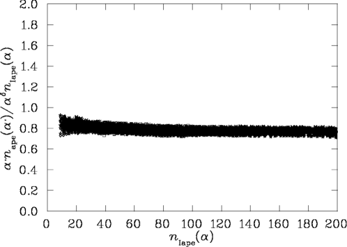
FIG. 25.: Illustration of the degree to which the relation Eq. (54) is satisfied for calibration of the action under APE and improved smearing. Here the entire data set is plotted.

C Calibration of Cooling and Smearing

In this section we apply the ansatz of equations Eq. (52) and Eq. (53) to relate the cooling and smearing algorithms. Fig. 26 displays results comparing cooling and standard APE smearing. For $\alpha$ as small as 0.1 it takes about 75 sweeps of APE smearing compared with 5 sweeps of cooling to arrive at an equivalent action. On the other end of the smearing fraction spectrum, we note the bands become very thick.

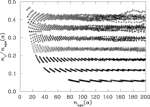
FIG. 26.: The ratio $\mbox{$n_{\rm{c}}$}/\mbox{$n_{\rm{ape}}(\alpha)$}$ versus $n_{\rm{ape}}(\alpha)$ for numerous action thresholds for the $16^{3}\times{32}$ lattice at $\beta=4.38$. From top down the data point bands correspond to $\alpha=0.7$, 0.6, 0.5, 0.4, 0.3, 0.2, and 0.1.

The calibration of these ratios indicates

$$\frac{\mbox{$n_{\rm{c}}$}}{\alpha\mbox{$n_{\rm{ape}}(\alpha)$}}=0.59(1),$$ (55)

in agreement with that obtained in [22] where the analysis was performed on unimproved gauge configurations. The reduction in ${\cal O}(a^{2})$ errors in the gauge field action affect both algorithms similarly such that the calibration of the relative smoothing rates remains unaltered.

Further broadening of the bands is observed when comparing improved cooling with APE smearing as illustrated in Fig. 27. The precision of improved cooling relative to APE smearing leads to very different smoothed configurations at this coarse lattice spacing of 0.165(2) fm. This indicates the algorithms are sufficiently different, that an accurate and meaningful calibration is impossible.

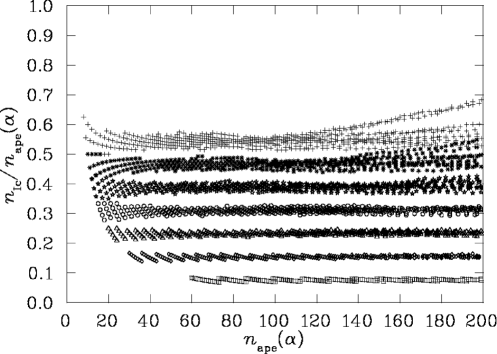
FIG. 27.: The ratio $\mbox{$n_{\rm{Ic}}$}/\mbox{$n_{\rm{ape}}(\alpha)$}$ versus $n_{\rm{ape}}(\alpha)$ for numerous action thresholds on the $16^{3}\times{32}$ lattice at $\beta=4.38$. From top down the data point bands correspond to $\alpha=0.7$, 0.6, 0.5, 0.4, 0.3, 0.2, and 0.1.

This effect is not observed when we pass to our fine lattice spacing as displayed in Fig. 28. We remind the reader that the thickness of the band for small numbers of smoothing sweeps is simply due to the ratio of small integers taken in plotting the $y$-axis values.

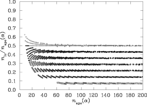
FIG. 28.: The ratio $\mbox{$n_{\rm{Ic}}$}/\mbox{$n_{\rm{ape}}(\alpha)$}$ versus $n_{\rm{ape}}(\alpha)$ for numerous action thresholds on the $24^{3}\times{36}$ lattice at $\beta=5.00$. From top down the data point bands correspond to $\alpha=0.7$, 0.6, 0.5, 0.4, 0.3, 0.2, and 0.1.

The real test of improved smearing is the extent to which the algorithm can preserve action associated with topological objects and thus maintain better agreement with more precise algorithms including cooling and improved cooling. Fig. 29 displays results for the calibration of improved cooling with improved smearing. Comparing these results for each smearing fraction, $\alpha$, with that for improved cooling and standard smearing in Fig. 27 reveals that the improved smearing algorithm, which was seen to be better than standard APE smearing algorithm does not perform as well as the improved cooling algorithm.

Similar results are seen in Fig. 30 where standard cooling is compared with improved smearing. Hence the annealing of the links in the process of cooling, where cooled links are immediately passed into the determination of the next cooled link, is key to the precision with which cooling can preserve topological structure.

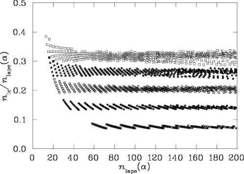
FIG. 29.: The ratio $\mbox{$n_{\rm{Ic}}$}/\mbox{$n_{\rm{Iape}}(\alpha)$}$ versus $n_{\rm{Iape}}(\alpha)$ for numerous action thresholds on the $16^{3}\times{32}$ lattice at $\beta=4.38$. From top down the data point bands correspond to $\alpha=0.5$, 0.4, 0.3, 0.2, and 0.1.

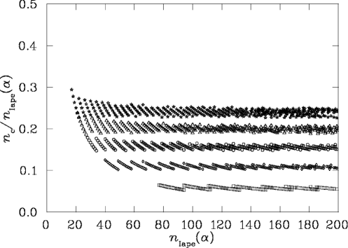
FIG. 30.: The ratio $\mbox{$n_{\rm{c}}$}/\mbox{$n_{\rm{Iape}}(\alpha)$}$ versus $n_{\rm{Iape}}(\alpha)$ for numerous action thresholds on the $16^{3}\times{32}$ lattice at $\beta=4.38$. From top down the data point bands correspond to $\alpha=0.5$, 0.4, 0.3, 0.2, and 0.1.

Calibration of the smoothing rates as measured by the action for the algorithms under investigation are summarized in Tables VI and VII. The entries describe the relative smoothing rate for the algorithm ratio formed by selecting an entry from the numerator column and dividing it by the heading of the denominator columns. The entry comparing APE smearing with itself reports the level to which the ansatz of equation Eq. (52) is satisfied. Similarly the entry comparing improved smearing with itself reports the level to which the ansatz of equation Eq. (53) is satisfied.

TABLE VI.: Calibration coefficients for various smoothing algorithms on the $16^{3}\times{32}$ lattice at $\beta=4.38$. Entries describe the relative smoothing rate for the algorithm ratio formed by selecting an entry from the numerator column and dividing it by the heading of the denominator columns. For example equation Eq. (55) corresponds to the first column of the third row.

	Denominator
Numerator	$\alpha\,\mbox{$n_{\rm{ape}}(\alpha)$}$	$\alpha^{\delta}\mbox{$n_{\rm{Iape}}(\alpha)$}$	$n_{\rm{c}}$	$n_{\rm{Ic}}$
$\alpha^{\prime}\,n_{\rm{ape}}(\alpha^{\prime})$	1.00(2)	0.81(2)	1.69(3)	1.30(2)
$\alpha^{\prime\delta}n_{\rm{Iape}}(\alpha^{\prime})$	1.25(3)	1.01(2)	2.13(5)	1.61(3)
$n_{\rm{c}}$	0.59(1)	0.47(1)	1	0.75(1)
$n_{\rm{Ic}}$	0.77(1)	0.62(1)	1.33(2)	1

TABLE VII.: Calibration coefficients for various smoothing algorithms on the $24^{3}\times{36}$ lattice at $\beta=5.00$. Entries describe the relative smoothing rate for the algorithm ratio formed by selecting an entry from the numerator column and dividing it by the heading of the denominator columns. For example equation Eq. (54) corresponds to the second column of the first row.

	Denominator
Numerator	$\alpha\,\mbox{$n_{\rm{ape}}(\alpha)$}$	$\alpha^{\delta}\mbox{$n_{\rm{Iape}}(\alpha)$}$	$n_{\rm{c}}$	$n_{\rm{Ic}}$
$\alpha^{\prime}\,n_{\rm{ape}}(\alpha^{\prime})$	1.00(2)	0.81(2)	1.64(2)	1.37(1)
$\alpha^{\prime\delta}n_{\rm{Iape}}(\alpha^{\prime})$	1.25(3)	1.01(2)	2.04(4)	1.67(3)
$n_{\rm{c}}$	0.611(9)	0.49(1)	1	0.84(1)
$n_{\rm{Ic}}$	0.734(8)	0.60(1)	1.19(1)	1

D Cooling versus Improved cooling.

Figure 31 reports a comparison of standard cooling with improved cooling on eleven configurations from the coarse $16^{3}\times{32}$ lattice. There the ratio $\mbox{$n_{\rm{c}}$}/\mbox{$n_{\rm{Ic}}$}<1$ confirms the expectation that standard cooling does not preserve action on the lattice as well as the ${\cal O}(a^{2})$-improved cooling. Fewer standard cooling sweeps are required to reach the same action threshold. Calibration of the algorithms appears plausible for the first 80 sweeps of improved cooling, after which the two algorithms smooth the configurations in very different manners. Any calibration at this lattice spacing is only very approximate beyond 80 sweeps of improved cooling where distinct configuration-dependent trajectories become visible. This result is contrasted by the analogous analysis on our fine $24^{3}\times{36}$ lattice illustrated in Fig. 32. While $\mbox{$n_{\rm{c}}$}/\mbox{$n_{\rm{Ic}}$}$ remains less than one, it is closer to one here than for the coarser lattice as one might expect.

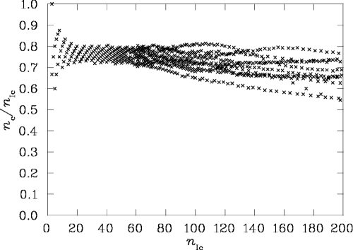
FIG. 31.: The ratio $\mbox{$n_{\rm{c}}$}/\mbox{$n_{\rm{Ic}}$}$ versus $n_{\rm{Ic}}$ for numerous action thresholds on the $16^{3}\times{32}$ lattice at $\beta=4.38$. The significant differences between the algorithms are revealed by the gauge-configuration dependence of the trajectories.

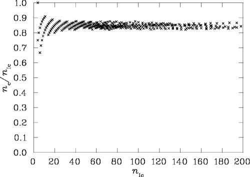
FIG. 32.: The ratio $\mbox{$n_{\rm{c}}$}/\mbox{$n_{\rm{Ic}}$}$ versus $n_{\rm{Ic}}$ for numerous action thresholds on the $24^{3}\times{36}$ lattice at $\beta=5.00$.

VII Conclusions

We have introduced an improved version of the APE smearing algorithm founded on the connection between cooling Eq. (32) and the projection of the APE smeared link back to the SU(3) gauge group via Eq. (49). This connection motivates the use of additional extended paths combined with the standard “staple” as governed by the action to reduce the introduction of ${\cal O}(a^{2})$ errors in the smearing projection process.

Clear signs of improvement are observed. For a given smearing fraction $\alpha$ defined in equation (46), improved smearing preserves the action better than standard APE smearing at each smearing sweep. At the same time improved smearing brings the improved topological charge to an integer value faster than standard APE smearing.

The extended nature of the “staple” in improved smearing reduces the stability regime for the smearing fraction. We found the improved smearing algorithm to be stable for $\alpha\leq 0.5$. At $\alpha=0.6$ the algorithm is unstable whereas standard APE smearing remains stable for $\alpha\leq 0.75$.

Given the wide variety of smoothing algorithms under investigation in the field of lattice gauge theory, we have cross calibrated the speed with which the algorithms remove action from the field configurations. In particular we have cross calibrated the smoothing rates of APE smearing at seven values of the smearing fraction; improved smearing at five values of the smearing fraction; cooling; and improved cooling. We explored smearing fractions in 0.1 intervals starting at $\alpha=0.1$.

The calibration has been investigated over a range of 200 sweeps for each smearing algorithm on ${\cal O}(a^{2})$-improved gauge field configurations. The results of this analysis allows one to make qualitative comparisons between cooling and smearing algorithms and in fact make quantitative comparisons of smearing algorithms with different smearing fractions on lattices as coarse as 0.165(2) fm. On our fine lattice where the lattice spacing is 0.077(1) fm, the calibration is quantitative in general.

We have found the relative smoothing rates are described via simple relationships as reported in Tables VI and VII for our coarse $16^{3}\times{32}$ and fine $24^{3}\times{36}$ lattices respectively. There the sensitivity of the calibration results on the lattice spacing may be reviewed. A noteworthy point is that we discovered a necessary correction to the APE smearing ratio rule [22] when improved smearing is considered. These algorithms may be calibrated via

$$\frac{n_{\rm{ape}}(\alpha^{\prime})}{\mbox{$n_{\rm{ape}}(\alpha)$}}=\frac{\alpha}{\alpha^{\prime}}\hskip 28.45274pt{\rm{and}}\hskip 28.45274pt\frac{n_{\rm{Iape}}(\alpha^{\prime})}{\mbox{$n_{\rm{Iape}}(\alpha)$}}=\left(\frac{\alpha}{\alpha^{\prime}}\right)^{\delta}\,$$ (56)

for APE smearing and improved smearing respectively. We find $\delta=0.914(1)$ without a significant dependence on the lattice spacing.

Having cross calibrated these smoothing algorithms, we now proceed to make contact with physical phenomena [4, 23, 24]. In particular, we note that it is possible to build in a length scale beyond which cooling does not affect the links [23]. It would be interesting to explore these techniques in the context of APE and Improved Smearing. Using a random walk argument, one can postulate a cooling radius

$$r_{\rm{cool}}=c\,\sqrt{\mbox{$n_{\rm{c}}$}}\,a\,,$$ (57)

where $a$ is the lattice spacing and $c$ is a constant independent of $\beta$ [24]. It has been shown that phenomena taken from simulation results with invariant $a\sqrt{\mbox{$n_{\rm{c}}$}}$ scale very well [24]. The effective range for APE smearing has been estimated using analytic methods [4]. For small smearing fraction, $\alpha$, the effective range is

$$r_{\rm{ape}}=\frac{1}{\sqrt{3}}\sqrt{\alpha\,\mbox{$n_{\rm{ape}}(\alpha)$}}\,a.$$ (58)

The product of $\alpha$ and $n_{\rm{ape}}(\alpha)$ defines $r_{\rm{ape}}$ in agreement with the results presented here. Eq. (56) indicates that this relation holds even for large $\alpha$. Results of our analysis contained in tables VI and VII allow one to link Eqs. (57) and (58) and thus determine the constant $c$. For sufficiently fine lattices $c$ is argued to be independent of $\beta$ [24] and this is already supported to some extent by the similarity of the entries in Tables VI and VII. For example, from Table VII, $\mbox{$n_{\rm{c}}$}={0.611(9)}\,\alpha\,\mbox{$n_{\rm{ape}}(\alpha)$}$ such that

$$r_{\rm{cool}}=\frac{1}{\sqrt{3(0.611(9))}}{\sqrt{\mbox{$n_{\rm{c}}$}}}\,a=0.739(5){\sqrt{\mbox{$n_{\rm{c}}$}}}\,a\,.$$ (59)

The effective range for other smoothing algorithms may be derived from Eq. (58) in a similarly straight forward manner.

Unfortunately a rigorous analysis of the scaling of the results of Tables VI and VII is not possible. We have clear evidence that the topology of Yang-Mills gauge fields cannot be reliably studied using the algorithms presented here on lattice spacings as coarse as 0.165(2) fm. Different algorithms lead to different topological charges, differing quite widely in some cases as reported in Figs. 11 and 12. Moreover, subtle differences in the cooling algorithms can lead to different topological charge determinations as illustrated in Figs. 3 and 4. As discussed in Sec. V A, the proximity of the dislocation thresholds of the algorithms to the typical size of instantons and variations in the threshold from one algorithm to another causes some (anti)instantons to survive under one algorithm, whereas they are removed under another.

In contrast, the fine $24^{3}\times{36}$ lattice results, where $a=0.077(1)$ fm, display excellent agreement among every smoothing algorithm considered. In this case it appears that the dislocation thresholds are smaller than the characteristic size of topological fluctuations such that the gauge fields are already sufficiently smooth to unambiguously extract the topology of the gauge fields.

As a final comparison of the smoothing algorithms, we provide a visual representation of a gauge field configuration after applying various smoothing algorithms. Figure 33 illustrates a rendering of the topological charge density for a slice of one of the fine $24^{3}\times{36}$ lattice configurations. While our calibration has been carried out by considering the total action of the gauge fields, the following analysis allows us to examine the extent to which the calibration is accurate at a microscopic level.

In Fig. 33, red shading indicates large positive topological charge density with decreasing density becoming yellow in color, while blue shading indicates large in magnitude, negative topological charge density decreasing in magnitude through the color green. Here cooling (a), improved cooling (b), APE smearing at $\alpha=0.70$ (c), APE smearing at $\alpha=0.30$ (d), improved smearing at $\alpha=0.50$ (e) and improved smearing at $\alpha=0.30$ (f), are compared at the number of smoothing iterations required for each algorithm to produce an approximately equivalent smoothed gauge field configuration. While Fig. b) for improved cooling differs somewhat due to round off in the sweep number, the remaining plots compare very favorably with each other. These visualizations confirm that the different smoothing algorithms considered in this investigation can be accurately related via the calibration analysis presented here and summarized in Tables VI and VII.

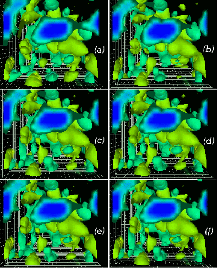
FIG. 33.: The topological charge density of a $24^{3}\times{36}$ lattice for fixed $x$ coordinate. The instantons (anti-instantons) are colored red to yellow (blue to green). Fig. a) shows the topological charge density after 9 cooling sweeps. Each of the following figures display the result of a different smoothing algorithm calibrated according to Table VII to reproduce as closely as possible the results depicted in Fig. a). Fig. b) illustrates the topological charge density after 11 sweeps of improved cooling. Fig.  c) shows the topological charge density after 21 APE smearing steps at $\alpha=0.70$. Fig. d) illustrates the topological charge density after 49 APE smearing steps at $\alpha=0.30$. In Fig. e) the topological charge density is displayed after 35 sweeps of improved smearing at $\alpha=0.50$. Finally, Fig. f) shows the topological charge density after 55 sweeps of improved smearing at $\alpha=0.30$. Apart from Fig. b) for improved cooling, which differs largely due to round off in the sweep number, all the plots compare very favorably with each other.

REFERENCES

- [1] M. Falcioni, M. Paciello, G. Parisi, B. Taglienti, Nucl. Phys. B251, [FS13] 624 (1985); M. Albanese et al, Phys. Lett. B192, 163 (1987).
- [2] T. DeGrand, et. al., Nucl. Phys. B547, 259 (1999); T. Blum, et. al., Phys. Rev. D 55, R1133 (1997).
- [3] T. DeGrand [MILC collaboration], Phys. Rev. D 60, 094501 (1999), hep-lat/9903006.
- [4] C. Bernard & T. DeGrand, Nucl. Phys. Proc. Suppl. 83-84, 845-847 (2000), hep-lat/9909083.
- [5] J. M. Zanotti, S. Bilson-Thompson, F. D. R. Bonnet, P. D. Coddington, D. B. Leinweber, A. G. Williams, J. B. Zhang, W. Melnitchouk, F. X. Lee, Submitted to Phys Rev. D, hep-lat/0110216.
- [6] W. Melnitchouk, S. Bilson-Thompson, F. D. R. Bonnet, P. D. Coddington, D. B. Leinweber, A. G. Williams, J. M. Zanotti, J. B. Zhang, F. X. Lee, hep-lat/0201005.
- [7] Waseem Kamleh, David Adams, Derek B. Leinweber, Anthony G. Williams, hep-lat/0112041.
- [8] W. Kamleh, D. Adams, D. B. Leinweber, A. G. Williams, hep-lat/0112042.
- [9] M. Campostrini, A. Di Giacomo, M. Maggiore, H. Panagopoulos & E. Vicari, Phys. Lett. B225, 403 (1989).
- [10] M. Campostrini, et al, Phys. Lett. B212, 206 (1988); M. Campostrini et al, Nucl. Phys. B17, 634 (1990); B. Alles, M. D’Elia & A. Di Giacomo, Nucl. Phys. B494, 281 (1997), hep-Lat/9605013.
- [11] B. Berg, Phys. Lett. B104, 475 (1981).
- [12] M. Teper, Phys. Lett. B180, 112 (1986); Nucl. Phys. B288, 589 (1987).
- [13] M. Teper, Phys. Lett. B162, 357 (1985); B171, 81,86 (1986).
- [14] E. M. Ilgenfritz et al, Nucl. Phys. B268, 693 (1986); J. Hoek et al, Nucl. Phys. B288, 589 (1987).
- [15] Margarita Garcia Perez, Antonio Gonzalez-Arroyo, Jeroen Snippe, Pierre van Baal, Nucl. Phys. B413, 535 (1994), hep-lat/9309009.
- [16] Philippe de Forcrand, Margarita G. Perez & Ion-Olimpiu Stamatescu, Nucl. Phys. B499, 409 (1997) hep-lat/9701012; P. de Forcrand, M. Garcia Perez, J. E. Hetrick & I. Stamatescu, hep-lat/9802017.
- [17] K. Symanzik, Nucl. Phys. B226, 187 (1983); ibid 205 (1983).
- [18] Y. Iwasaki, K. Kanaya, T. Kaneko, T. Yoshie, Phys. Rev. D 56, 151 (1997), hep-lat/9610023.
- [19] Tetsuya Takaishi, Phys. Rev. D 54, 1050 (1996).
- [20] QCD-TARO Collaboration (T. Umeda et al.), Nucl. Phys. Proc. Suppl. 73, 924 (1999), hep-lat/9809086.
- [21] Thomas DeGrand, Anna Hasenfratz, Tamas G. Kovacs, Nucl.Phys. B520, 301 (1998), hep-lat/9711032.
- [22] F. D. R. Bonnet, P. Fitzhenry, D. B. Leinweber, M. R. Stanford & A. G. Williams, Phys. Rev. D 62, 094509 (2000), hep-lat/0001018.
- [23] Margarita Garcia Perez, Owe Philipsen, Ion-Olimpiu Stamatescu, Nucl. Phys. B551 293 (1999), hep-lat/9812006.
- [24] A. Ringwald, F. Schrempp, Phys. Lett. B459 249 (1999), hep-lat/9903039.
- [25] N. Cabibbo & E. Marinari, Phys. Lett. B119, 387 (1982).
- [26] F. D. R. Bonnet, D. B. Leinweber & A. G. Williams, J. Comput. Phys. 170, 1-17 (2001), hep-lat/0001017.
- [27] B. Sheikholeslami & R. Wohlert, Nucl. Phys. B259, 572 (1985).
- [28] M. Luscher & P. Weisz, Commun. Math. Phys. 97, 59 (1985), Erratum-ibid. 98, 433 (1985).
- [29] Y. Iwasaki & T. Yoshie, Phys. Lett. B131, 159 (1983).
- [30] S. Bilson-Thompson, F. D. R. Bonnet, D. B. Leinweber & A. G. Williams, hep-lat/0112034 and ibid, “Topological Charge and Action Operators from a Highly–Improved Lattice field–Strength Tensor”. To be Submitted to Phys. Rev. D, ADP-01-50/T482.
- [31] G. P. Lepage, “Redesigning lattice QCD”, in Perturbative and Nonperturbative Aspects of Quantum Field Theory, (Proc. of 35th International Universitätswochen für Ken–und Teichenphysik, Schladming, Austria, March 2–9, 1996), p. 1-45, (Springer–Verlag Berlin Heidelberg, 1997), hep-lat/9607076.
- [32] J. E. Hetrick & P. de Forcrand, Nucl. Phys. B (Proc. Suppl.) 63, 838 (1998), hep-lat/9710003.