Renormalization Constants using Quark States in Fixed Gauge LA-UR-01-0355

Abstract

We present a status report on our calculation of the renormalization constants for the quark bilinears in quenched $O(a)$ improved Wilson theory at $\beta=6.4$ using quark states in Landau gauge.

1 INTRODUCTION

One of the leading uncertainties in current lattice calculations comes from the renormalization constants necessary to relate the lattice currents to those in some continuum renormalization scheme. Until recently, the most commonly used method for determining these was 1-loop perturbation theory. In the last few years a non-perturbative method based on axial and vector Ward identities has been developed [1]. This allows the determination of all scale invariant renormalization constants, and all $O(a)$ improvement constants for bilinear operators. For the remaining bilinears and four fermion operators that arise in the weak effective Hamiltonian, the method of choice uses external quark states in Landau gauge [2]. This defines the renormalization constants in the RI or MOM scheme, in which the value of the renormalized operators is specified at some fixed momentum for the external quarks.

In this talk we present a status report of our calculations using quark states in Landau Gauge at $\beta=6.4$.

The calculation involves two quantities: the quark propagator, $S(p)$ and the three point functions, $C^{\Gamma}(p,q)$,

$$S(p) = \sum_{y}\left\langle\psi(y)\mathord{\overline{\psi}}(0)\right\rangle\times e^{ipy}$$ (1)

$$C^{\Gamma}(p,q) = \sum_{xy}\left\langle\psi(y)\mathord{\overline{\psi}}(0)\Gamma\psi(0)\mathord{\overline{\psi}}(x)\right\rangle$$ (2)

$$\qquad\times e^{ip(x-y)}e^{-iq(x+y)/2}\,,$$

where $\Gamma$ is an element of the Clifford algebra, $\psi$ is the fermion field, and we only consider flavor non-singlet operators. In terms of these we define

$$\Gamma^{\Sigma} = \mathop{\rm Im}\frac{\partial{S(p)^{-1}}}{{\partial{\mathchoice{{{\hbox to5.03125pt{\hss$\displaystyle/$\hss}\hbox{$\displaystyle p$}}}}{{{\hbox to5.03125pt{\hss$\textstyle/$\hss}\hbox{$\textstyle p$}}}}{{{\hbox to3.52188pt{\hss$\scriptstyle/$\hss}\hbox{$\scriptstyle p$}}}}{{{\hbox to2.51563pt{\hss$\scriptscriptstyle/$\hss}\hbox{$\scriptscriptstyle p$}}}}}}}$$ (3)

$$\Gamma^{m} = \mathop{\rm Re}\frac{\partial{S(p)^{-1}}}{{\partial{m}}}$$ (4)

$$\Gamma^{\Gamma} = S(p)^{-1}C^{\Gamma}(p,0)S(p)^{-1}\,.$$ (5)

The RI scheme then corresponds to choosing a momentum $p_{\mu}$ (and mass $m=0$) at which the renormalized inverse propagator and the renormalized truncated three point functions have their tree level values:

$$\Gamma^{\Sigma}_{R} \equiv Z_{\psi}^{-1}\Gamma^{\Sigma}\qquad=1$$ (6)

$$\Gamma^{m}_{R} \equiv Z_{\psi}^{-1}Z_{m}^{-1}\Gamma^{m}=1$$ (7)

$$\Gamma^{\Gamma}_{R} \equiv Z_{\psi}^{-1}Z_{\Gamma}\Gamma^{\Gamma}\ \ \,=\Gamma\,.$$ (8)

These equations, thus, define the wave function renormalization constant, $Z_{\psi}$, the mass renormalization constant, $Z_{m}$, and the renormalization constants for the bilinears, $Z_{\Gamma}$. The resulting renormalized quantities are then also the same those in the continuum RI scheme at renormalization scale $\mu^{2}=p^{2}$.

The most common scheme in which phenomenological results are presented is the $\overline{MS}$, which can be obtained from the RI scheme results by a perturbative calculation in the continuum. However, it is worth noting that the RI scheme does not respect the axial ward identities, and this breaking of the ward identity cannot be accounted for in the connection between RI and $\overline{MS}$ using perturbation theory  [2]. Specifically, these identities require that

$$\gamma_{5}\mathbin{}(1+m_{R}\frac{\partial{}}{{\partial{m_{R}}}})\Gamma^{P}_{R}=-\Gamma^{m}_{R}$$ (9)

$$\gamma_{5}\mathbin{}(1-q_{\mu}\frac{\partial{}}{{\partial{q_{\mu}}}})\Gamma^{A}_{R}=-\Gamma^{\Sigma}_{R}$$ (10)

at $q_{\mu}=m=0$, where $m_{R}=Z_{m}m$ is the renormalized mass and $P$ and $A$ are the pseudoscalar and axial bilinears. Fortunately, the derivative terms in these equations, which contribute due to the Goldstone pole at zero quark mass arising out of chiral symmetry breaking, become irrelevant when the renormalization scale $\mu$ is large compared to the scale of chiral symmetry breaking [2]. On the other hand lattice discretization errors become large for $pa$ larger than unity. Thus, the method relies on the existence of an intermediate window in which these two artifacts are small.

2 DISCRETIZATION EFFECTS

In the lattice regularization scheme operators receive power corrections which involve higher dimension operators. This is a consequence of the hard cutoff, $i.e.$ the lattice spacing $a$. In addition, because the RI scheme is defined in a fixed gauge, gauge-invariant and gauge-dependent operators, in general, mix. Application of BRS symmetry shows [3] that, at $O(a)$ and $q=0$, the only corrections to $\mathord{\overline{\psi}}\Gamma\psi$ are gauge invariant and of the form $\mathord{\overline{\psi}}(\mathord{\mathop{\cal W}\limits^{\leftarrow}}\Gamma+\Gamma\mathord{\mathop{\cal W}\limits^{\rightarrow}})\psi$, where ${\cal W}$ is the Dirac operator and this correction vanishes by the equation of motion, $\mathord{\overline{\psi}}\mathord{\mathop{\cal W}\limits^{\leftarrow}}=\mathord{\mathop{\cal W}\limits^{\rightarrow}}\psi=0$. Such a correction term, therefore, does not affect the on-shell matrix elements of these operators, but does contribute to the momentum space correlators in Eq. 2 as these involve contributions from points where the operator and the fermion sources overlap.

At $O(a)$ only $\mathchoice{{{\hbox to11.35695pt{\hss$\displaystyle/$\hss}\hbox{$\displaystyle\mathord{\mathop{D}\limits^{\rightarrow}}$}}}}{{{\hbox to11.35695pt{\hss$\textstyle/$\hss}\hbox{$\textstyle\mathord{\mathop{D}\limits^{\rightarrow}}$}}}}{{{\hbox to7.98985pt{\hss$\scriptstyle/$\hss}\hbox{$\scriptstyle\mathord{\mathop{D}\limits^{\rightarrow}}$}}}}{{{\hbox to6.27846pt{\hss$\scriptscriptstyle/$\hss}\hbox{$\scriptscriptstyle\mathord{\mathop{D}\limits^{\rightarrow}}$}}}}-m$ part of $\mathord{\mathop{\cal W}\limits^{\rightarrow}}$ contributes to the mixing; consequently, the scalar density and the vector current mix, as do the axial current and the tensor density. The pseudoscalar current receives only multiplicative corrections at this order. At higher orders, the violation of rotational and Lorentz symmetries show up, and different components of $V_{\mu}$, $A_{\mu}$, and $T_{\mu\nu}$ mix amongst themselves.

To take the $O(a)$ mixing into account, Eq. 8 is modified to

$$\Gamma^{\Gamma}_{R} \equiv Z_{\psi}^{-1}Z_{\Gamma}\Gamma^{\Gamma}_{I}$$ (11)

$$\Gamma^{\Gamma}_{I} \equiv \Gamma^{\Gamma}+c^{\prime}_{\Gamma}(\Gamma S^{-1}+S^{-1}\Gamma)\,,$$ (12)

where $c^{\prime}_{\Gamma}$ is determined by the requirement that

$$\mathop{\rm Tr}\Gamma^{\Gamma}_{I}\Gamma^{\prime}=0\,,$$ (13)

where $\Gamma^{\prime}=S$, $V$, $T$, and $A$ for $\Gamma=V$, $S$, $A$, and $T$ respectively. Unfortunately, as stated above, there is no analogous condition to determine $c^{\prime}_{P}$ since $\gamma_{5}S^{-1}+S^{-1}\gamma_{5}\propto\gamma_{5}$. An illustration of the magnitude of the mixing is given in Table 1 from which the $c_{\Gamma}^{\prime}$ are determined. Similarly, at $O(a)$, the propagator gets corrections

$$S_{I}(p)=(1-2ac^{NGI}_{\psi}\mathchoice{{{\hbox to5.03125pt{\hss$\displaystyle/$\hss}\hbox{$\displaystyle p$}}}}{{{\hbox to5.03125pt{\hss$\textstyle/$\hss}\hbox{$\textstyle p$}}}}{{{\hbox to3.52188pt{\hss$\scriptstyle/$\hss}\hbox{$\scriptstyle p$}}}}{{{\hbox to2.51563pt{\hss$\scriptscriptstyle/$\hss}\hbox{$\scriptscriptstyle p$}}}})S(p)-2ac^{\prime}_{\psi}\,,$$ (14)

where $c^{NGI}_{\psi}$ and $c^{\prime}_{\psi}$ are the gauge-variant and gauge-invariant corrections respectively. Methods to determine a combination of these coefficients have been discussed in Ref. [4] and we do not repeat the discussion here.

3 LATTICE PARAMETERS AND METHODOLOGY

Our pilot calculation utilizes 60 lattices at $\beta=6.4$ which corresponds to a lattice scale of $a^{-1}\approx 3.85{\rm GeV}$ [5] and a critical hopping parameter $\kappa_{c}\approx 0.135796$ [6]. The quark propagators were inverted at seven values of $\kappa=0.1280$, 0.1294, 0.1308, 0.1324, 0.1334, 0.1343, and 0.1348 using a clover coefficient value of $c_{SW}=1.526$ [7]. Unless stated otherwise, we shall only consider momenta such that all components are less than $\pi/4$.

The truncated three-point functions were calculated and projected on the Clifford basis. As shown in Tab. 1, the data, in addition to the expected terms, shows $O(a)$ mixing ($S\leftrightarrow V_{i}$), and the two $O(a^{2})$ effects: mixing ($V_{3}\leftrightarrow V_{4}$) and the difference between the terms parallel and perpendicular to the momentum. The latter effect is due to the violation of rotational symmetry. As mentioned in the previous section, we correct for the $O(a)$ mixings by determining the $c^{\prime}_{\Gamma}$, but, at $pa\sim 1$, the approximately $2\%$ violation of rotational symmetry and $0.6\%$ mixings due to higher order effects survive.

Table 1: The various Clifford projections of the truncated 3-point functions corresponding to the scalar and vector bilinears at $\kappa=0.1294$ and $pa=(0,0,3,3)\times\pi/16$.

operator	projection	value
$S$	$1$	$1.180(5)$
	$\gamma_{3}$	$0.059(3)$
	$\gamma_{4}$	$0.059(3)$
$V_{1}$	$\gamma_{1}$	$1.067(5)$
$V_{2}$	$\gamma_{2}$	$1.067(5)$
$V_{3}$	$\gamma_{3}$	$1.086(3)$
	$1$	$0.019(2)$
	$\gamma_{4}$	$0.006(1)$
$V_{4}$	$\gamma_{4}$	$1.083(3)$
	$1$	$0.021(2)$
	$\gamma_{3}$	$0.006(1)$

To calculate the wave function renormalization, we Fourier transform the inverse propagator,

$$S^{-1}(p)=\sum_{\{n\}}a_{\{n\}}\prod_{\mu}\sin n_{\mu}p_{\mu}\,,$$ (15)

and calculate the derivative in Eq. 3 analytically:

$$\Gamma^{\Sigma}=\frac{1}{4}\sum_{\mu}\frac{1}{4}\mathop{\rm Tr}\gamma_{\mu}\sum_{\{n\}}n_{\mu}a_{\{n\}}\prod_{\nu}\cos n_{\nu}p_{\nu}\,.$$ (16)

We expect large $O(a^{2})$ discretization errors for the following reason. At tree level $\Gamma^{\Sigma}=(1/4)\sum_{\mu}cosp_{\mu}$, which deviates from unity by $\sim 15\%$ at $pa\sim 1$. To correct for this artifact, we divide the calculated $\Gamma^{\Sigma}$ by this tree-level contribution, and use the resulting $\Gamma^{\Sigma}$ in Eq. 7 to calculate $Z_{\psi}$. Note that such a determination of $Z_{\psi}$ contains residual $O(a)$ errors stemming from the use of the uncorrected propagator.

4 RESULTS

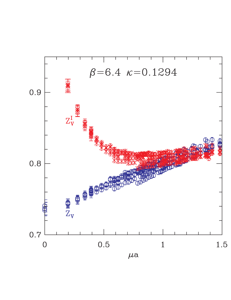
Figure 1: The improved (crosses) and unimproved (circles) vector renormalization constants as a function of the renormalization scale.

In Fig. 1, we show the effect of improvement for the vector current, $i.e.$ removing the $O(a)$ term by calculating $c^{\prime}_{V}$. In the absence of discretization errors, the calculated $Z_{V}$ should be independent of the scale $\mu$ except for non-perturbative terms. Non-perturbative terms are expected to fall off as $1/\mu^{2}$ at large $\mu$ [2]. Instead the uncorrected data shows a linear rise, $Z_{V}$ changing by $\sim 5\%$ between $0.8<\mu a<1.5$. In contrast, the $O(a)$ corrected quantity is constant over this range of $\mu a$. There is roughly $2-3\%$ uncertainty in $Z_{V}$ coming from the variation between different Lorentz components and different combinations of momenta in this range.

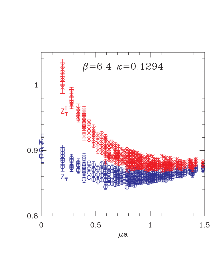
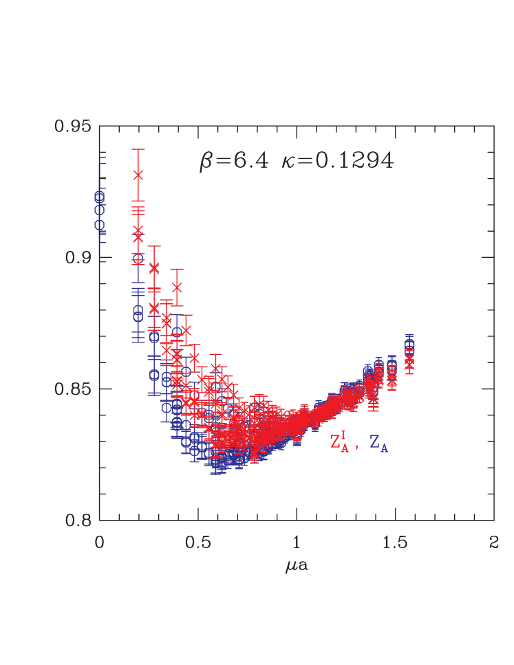
Figure 2: The improved (crosses) and unimproved (circles) tensor renormalization constants as a function of the renormalization scale.

Figure 3: The improved (crosses) and unimproved (circles) axial vector renormalization constants as a function of the renormalization scale.

Fig. 3 shows that the behavior of tensor renormalization constant, $Z_{T}$, is qualitatively similar: the much smaller linear rise of the unimproved $Z_{T}$ for $\mu a>0.8$ is removed by the improvement. Finally, we show the behavior of the axial vector channel in Fig. 3. We do not observe any improvement in $Z_{A}$ and the data do not show a window in which it is independent of $\mu a$.

5 DISCUSSIONS

Since we have not finished the analysis, we end with a few qualitative statements. (i) The $O(a)$ errors induced due to mixing with the equation of motion operators can be corrected for by calculating $c^{\prime}_{\Gamma}$. These $c^{\prime}_{\Gamma}$ can then be compared with those evaluated using the axial Ward identity [1]. (ii) At $\beta=6.4$, the presence of non-perturbative corrections forces us to work at $\mu a\sim 0.8$ or higher to determine the renormalization constants. At these large momenta, the $O(a^{2})$ errors are only slightly smaller than the $O(a)$ errors, and it is important to ascertain whether our attempts to correct the latter introduce unacceptably large $O(a^{2})$ errors. In particular, the correction terms in Eq. 12 involve the inverse propagator, and an $O(a)$ improvement in the propagator used in this equation changes results at $O(a^{2})$. The use of a suitably improved propagator would make the $O(a)$ correction term vanish in the chiral limit except for non-perturbative effects that fall off as $1/p^{2}$. In practice, as already noted in Ref. [4], the bare inverse propagator has large $O(ap^{2})$ corrections even in the chiral limit, and hence our improvement term does not vanish there.

To summarize, $O(a^{2})$ corrections are large and, at present, uncontrolled. We are investigating ways to improve the calculation and the results of this study will be reported elsewhere.

References

- [1] T. Bhattacharya, R. Gupta, W. Lee, and S. Sharpe, to appear in Phys. Rev. D. [hep-lat/0009038] and references therein.
- [2] G. Martinelli, C. Pittori, C.T. Sachrajda, M.Test, and A. Vladikas, Nucl. Phys. B445 (1995) 81. [hep-lat/9411010]
- [3] G. Martinelli, et al., Phys. Lett. B411 (1997) 141. [hep-lat/9705018]
- [4] D. Becirevic, V. Giménez, V. Lubicz, and G. Martinelli, Phys. Rev. D61 (2000) 114507. [hep-lat/9909082]
- [5] M. Göckeler, et al, Phys. Rev. D62 (2000) 054504. [hep-lat/9908005]
- [6] Calculated from data in Ref. [5].
- [7] M. Lüscher, S. Sint, R. Sommer, and P. Weisz, Nucl. Phys. B478 (1996) 365. [hep-lat/9605038]