BI-TP 2001/07
May 2001

Finite-size-scaling functions for
$3d$ $O(4)$ and $O(2)$ spin models and QCD
J. Engels$\,{}^{\rm a}$, S. Holtmann$\,{}^{\rm a}$, T. Mendes$\,{}^{\rm b}$ and T. Schulze$\,{}^{\rm a}$

^aFakultät für Physik, Universität Bielefeld, D-33615 Bielefeld, Germany

^bIFSC-USP, Caixa postal 369, 13560-970 São Carlos SP, Brazil

Abstract

We calculate numerically universal finite-size-scaling functions for the three-dimensional $O(4)$ and $O(2)$ models. The approach of these functions to the infinite-volume scaling functions is studied in detail on the critical and pseudocritical lines. For this purpose we determine the pseudocritical line in two different ways. We find that the asymptotic form of the finite-size-scaling functions is already reached at small values of the scaling variable. A comparison with QCD lattice data for two flavours of staggered fermions shows a similar finite-size behaviour which is compatible with that of the spin models.

PACS : 64.60.C; 75.10.H; 12.38.Gc

Keywords: Finite-size-scaling function; $O(N)$ model; Quantum chromodynamics

 
E-mail: engels,holtmann,tschulze@physik.uni-bielefeld.de; mendes@if.sc.usp.br

1 Introduction

At finite temperature quantum chromodynamics (QCD) undergoes a chiral phase transition. For two degenerate light-quark flavours this transition is supposed to be of second order in the continuum limit and to belong to the same universality class as the $3d$ $O(4)$ model [1]-[3]. QCD lattice data have therefore been compared to the universal $O(4)$ scaling function [4]-[6]. The scaling function or equation of state describes the system in the thermodynamic limit, that is for $V\rightarrow\infty$. It was first determined numerically in Ref. [7] and later studied in more detail in Ref. [8]. Lattice results for Wilson fermions [9, 10] seem to agree quite well with the predictions, though for the Wilson action the chiral symmetry is only restored in the continuum limit. In the staggered formulation of QCD a part of the chiral symmetry is remaining even for finite lattice spacing, and that is $O(2)$. Nevertheless, comparisons with $O(4)$ or even $O(2)$ scaling functions [11] have up to now not confirmed the expectations for staggered fermions [12]-[14]. Among the many arguments [14, 15], which have been put forward to explain this failure, one is obvious, namely, that lattice QCD simulations are still performed on relatively small volumes and therefore will show substantial finite size effects. More adequate tests may be carried out, if universal finite-size-scaling functions for the $O(N)$-spin models are available. This exactly is the aim of the paper: the calculation of finite-size-scaling functions for the $O(4)$ and $O(2)$ models and a corresponding test of QCD lattice data.

We shall make extensive use of the results of two of our papers: a study of the three-dimensional $O(4)$ model, Ref. [8], and another one for the $O(2)$ model, Ref. [11]. There we determined the respective equations of state. In the following we briefly review the equations which are relevant for this paper.

The $O(N)$-invariant nonlinear $\sigma$-models, which we investigate are defined by

$$\beta\,{\cal H}\;=\;-J\,\sum_{<i,j>}{\bf S}_{i}\cdot{\bf S}_{j}\;-\;{\bf H}\cdot\,\sum_{i}{\bf S}_{i}\;,$$ (1)

where $i$ and $j$ are nearest-neighbour sites on a $d-$dimensional hypercubic lattice, and ${\bf S}_{i}$ is an $N$-component unit vector at site $i$. It is convenient to decompose the spin vector ${\bf S}_{i}$ into a longitudinal (parallel to the magnetic field ${\bf H}$) and a transverse component

$${\bf S}_{i}\;=\;S_{i}^{\parallel}{\bf\hat{H}}+{\bf S}_{i}^{\perp}~{}.$$ (2)

The order parameter of the system, the magnetization $M$, is then the expectation value of the lattice average $S^{\parallel}$ of the longitudinal spin component

$$M\;=\;<\!\frac{1}{V}\sum_{i}S_{i}^{\parallel}>\;=\;<S^{\parallel}>~{}.$$ (3)

There are two types of susceptibilities: the longitudinal susceptibility is defined as usual by the derivative of the magnetization, whereas the transverse susceptibility corresponds to the fluctuation of the lattice average ${\bf S}^{\perp}$ of the transverse spin per component

$$\chi_{L}\!\! \!=\! \!\!{\partial M\over\partial H}\;=\;V(<{S^{\parallel}}^{2}>-M^{2})~{},$$ (4)

$$\chi_{T}\!\! \!=\! \!\!{V\over N-1}<{{\bf S}^{\perp}}^{2}>\;=\;{M\over H}~{}.$$ (5)

We do not discuss here as in [8] and [11] the singularities of the susceptibilities on the coexistence line which are due to the Goldstone modes. We simply note, that the general Widom-Griffiths form of the equation of state [16], which describes the critical behaviour of the magnetization in the vicinity of $T_{c}$, is compatible with these singularities. It is given by

$$y\;=\;f(x)\;,$$ (6)

where

$$y\equiv h/M^{\delta},\quad x\equiv t/M^{1/\beta}.$$ (7)

The variables $t$ and $h$ are the normalized reduced temperature $t=(T-T_{c})/T_{0}$ and magnetic field $h=H/H_{0}$. We take the usual normalization conditions

$$f(0)=1,\quad f(-1)=0~{}.$$ (8)

The critical exponents $\delta$ and $\beta$ appearing in Eqs. 6 and 7 specify all the other critical exponents

$$d\nu=\beta(1+\delta),\quad\gamma=\beta(\delta-1),\quad\nu_{c}=\nu/\beta\delta~{}.$$ (9)

Possible irrelevant scaling fields and exponents are however not taken into account in Eq. 6, the function $f(x)$ is universal. Another way to express the dependence of the magnetization on $t$ and $h$ is

$$M\;=\;h^{1/\delta}f_{G}(t/h^{1/\beta\delta})~{},$$ (10)

where $f_{G}$ is a scaling function. This type of scaling equation is used for comparison to QCD lattice data. The scaling forms in Eqs. (6) and (10) are clearly equivalent, since the variables $x$ and $y$ are related to the scaling function $f_{G}$ and its argument by

$$y\;=\;f_{G}^{-\delta}\;,\quad x\;=\;(t/h^{1/\beta\delta})\,f_{G}^{-1/\beta}\;.$$ (11)

In Refs. [8] and [11] we had parametrized the equation of state by a combination of a small-$x$ (low temperature) form $x_{s}(y)$, which was inspired by the approximation of Wallace and Zia [17] close to the coexistence line ($x=-1;~{}y=0$)

$$x_{s}(y)+1\;=\;({\widetilde{c}_{1}}\,+\,{\widetilde{d}_{3}})\,y\,+\,{\widetilde{c}_{2}}\,y^{1/2}\,+\,{\widetilde{d}_{2}}\,y^{3/2}\;,$$ (12)

and a large-$x$ (high temperature) form $x_{l}(y)$ derived from Griffiths’s analyticity condition[16]

$$x_{l}(y)\;=\;a\,y^{1/\gamma}\,+\,b\,y^{(1-2\beta)/\gamma}~{}.$$ (13)

${\widetilde{c}_{1}}\,+\,{\widetilde{d}_{3}}$	${\widetilde{c}_{2}}$	${\widetilde{d}_{2}}$	$a$	$b$	$y_{0}$	$p$
0.345(12)	0.674(08)	-0.023(5)	1.084(6)	-0.994(109)	10.0	3	$O(4)$
0.352(30)	0.592(10)	0.056	1.260(3)	-1.163(20)	$\;~{}3.5$	6	$O(2)$

Table 1: Parameters of the fits to the scaling functions for $O(4)$ and $O(2)$.

$\beta$	$\delta$	$\gamma$	$\nu$	$\nu_{c}$	$J_{c}$	$T_{0}$	$H_{0}$
0.380	4.86	1.4668	0.7423	0.4019	0.93590	1.093	5.08	$O(4)$
0.349	4.7798	1.3192	0.6724	0.4031	0.454165	1.18	1.11	$O(2)$

Table 2: Critical parameters used in the $O(4)$ [8] and $O(2)$ [11] calculations.

The two parts can be interpolated smoothly by an ansatz of the kind

$$x(y)\;=\;x_{s}(y)\,\frac{y_{0}^{p}}{y_{0}^{p}+y^{p}}\,+\,x_{l}(y)\,\frac{y^{p}}{y_{0}^{p}+y^{p}}~{},$$ (14)

from which the total scaling function is obtained. In Table 1 the parameters of these fits are listed. Two remarks are necessary here: for $O(2)$ the coefficient ${\widetilde{d}_{2}}$ was fixed by the normalization $y(0)=1$, that is ${\widetilde{d}_{2}}=1-({\widetilde{c}_{1}}+{\widetilde{d}_{3}}+{\widetilde{c}_{2}})$, and in the $O(4)$ case the coefficient $b$ was incorrectly cited in Ref. [8]. Of course, the scaling functions are not independent of the critical points, amplitudes and exponents, which had been used in their determination. For completeness we therefore give in Table 2 the relevant input.

2 Finite-Size-Scaling Functions

The general form of the finite-size-scaling function for the magnetization is given by

$$M=L^{-\beta/\nu}\Phi(tL^{1/\nu},hL^{1/\nu_{c}},L^{-\omega})~{},$$ (15)

that is, we have a function of three (or even more) variables, which describes the dependence of the magnetization on the thermal, magnetic and possible irrelevant scaling fields and the characteristic linear extension $L$ of the volume. Here we have specified only the leading irrelevant scaling field proportional to $L^{-\omega}$, with $\omega>0$. A universal scaling function is obtained, when we expand the function $\Phi$ in $L^{-\omega}$ and consider the first term only

$$M=L^{-\beta/\nu}\Phi_{0}(tL^{1/\nu},hL^{1/\nu_{c}})+\dots~{}.$$ (16)

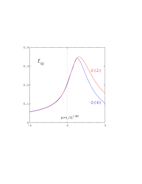
Figure 1: The scaling function $f_{G\chi}(z)$ of the longitudinal susceptibility for the $O(4)$ and $O(2)$ models.

The function $\Phi_{0}$ still depends on two variables. In order to handle the two-variable dependence of $\Phi_{0}$ in an economic way, we consider in the following paths in the $(t,h)$-plane defined by fixed values of $z=th^{-1/\beta\delta}$. At fixed $z$ we can express one of the two variables of Eq. (16) by $z$ and the other variable, leaving us with a function of one variable only

$$M=L^{-\beta/\nu}Q_{z}(hL^{1/\nu_{c}})+\dots~{},$$ (17)

where $Q_{z}$ is again universal. The procedure has the additional advantage that $z$ is the argument of the scaling function $f_{G}$ of Eq. (10), thus requiring only one point of $f_{G}$ to calculate the asymptotic form $Q_{z,\infty}$ of the finite-size-scaling function $Q_{z}$

$$Q_{z}\rightarrow Q_{z,\infty}=f_{G}(z)(hL^{1/\nu_{c}})^{1/\delta}\quad\mbox{for}\quad L\rightarrow\infty~{}.$$ (18)

Examples of lines of fixed $z$ are the critical line where $z=0$ and the pseudocritical line, the line of peak positions of the susceptibility $\chi_{L}$ in the $(t,h)$-plane for $V\rightarrow\infty$. There are two ways to find that value of $z$ for $O(N)$, which corresponds to the pseudocritcal line. One way amounts to locating the peak positions of $\chi_{L}$ as a function of the temperature at different fixed small values of the magnetic field on lattices with increasing size $L^{3}$. This method has been used in QCD. For staggered fermions the pseudocritical line thus found shows up to now the most convincing agreement with the $O(N)$ models. The scaling function offers a more elegant way to determine the pseudocritical line. Since $\chi_{L}$ is the derivative of $M$

$$\chi_{L}={\partial M\over\partial H}={h^{1/\delta-1}\over H_{0}}f_{G\chi}(z)~{},$$ (19)

its scaling function $f_{G\chi}(z)$ can be calculated directly from $f_{G}(z)$

$$f_{G\chi}(z)={1\over\delta}\left(f_{G}(z)-{z\over\beta}f_{G}^{\prime}(z)\right)~{}.$$ (20)

Evidently, the maximum of $\chi_{L}$ at fixed $h$ and varying $t$ is at the peak position $z_{p}$ of $f_{G\chi}(z)$ and $z_{p}$ is another universal quantity. In Fig. 1 we show the result for $f_{G\chi}(z)$ from Eq. (20) using the scaling functions $f_{G}$ for $O(4)$ and $O(2)$ as obtained from Table 1. In this calculation we have interpolated the small-$x$ and large-$x$ derivatives $y(dx/dy)$ to smooth the result. We see from Fig. 1 that there is a relatively broad peak at positive $z$ and we can read off the value of $z_{p}$ for the two models. They are listed in Table 3 together with the peak height of $f_{G\chi}$. It is instructive to use the

Scaling function		$L=24$ to 96
$z_{p}$	$f_{G\chi}(z_{p})$	$z_{p}$
$1.33\pm 0.05$	0.341(1)	$1.35\pm 0.10$	$O(4)$
$1.56\pm 0.10$	0.350(1)	$1.65\pm 0.10$	$O(2)$

Table 3: The peak position and height of the scaling function $f_{G\chi}\,$, and $z_{p}$ from calculations on lattices with size $L=24$ to 96.

QCD method for $z_{p}$ determination on finite lattices as well. For that purpose we have calculated at eight values of the magnetic field on lattices of size $L=24,\dots,96$ the peak positions and heights for $O(4)$. The infinite volume estimates for the two quantities are compared in Fig. 2 and Table 3 to the results from the scaling function. We observe in Fig. 2a that the agreement is very good for the peak positions at small $h$. At larger $h$ there is a slight tendency towards somewhat higher pseudocritical temperatures than expected from the fixed $z$ relation between $t$ and $h$ at the peak. The peak heights in Fig. 2b on the other hand are following nicely the prediction $\chi_{L}=0.244H^{1/\delta-1}$ from the scaling function for all $H$. We have obtained similar results for $O(2)$ at two values of $H$. Fig. 2a contains also lines for several other fixed $z$ values to give a better overview of the $(t,h)$-plane. As examples we shall investigate in the next two subsections the finite-size behaviour of the magnetization on the lines $z=0$ and $z=z_{p}$.

2.1 Finite-Size Scaling in the $O(4)$ Model

Our simulations are done on three-dimensional lattices with periodic boundary conditions and linear extensions $L$ up to 120. We use the same cluster algorithm as in Refs. [8, 11]. Let us first consider the critical line in $O(4)$. In Fig. 4b of Ref. [8] we had observed, that there are essentially no corrections to scaling on the critical line. Here we extend this investigation by including more points at higher and also very

Figure 2: (a) Lines of fixed $z=0.5,1,1.5,2$ (dashes), the pseudocritical line (solid) at $z_{p}=1.33\pm 0.05$ and measured peak positions (squares). (b) the peak height of $\chi_{L}$ as a function of $H$, measured (squares) and from the scaling funtion (solid line). Both parts of the figure refer to the $O(4)$ model.

Figure 3: (a) Finite-size scaling of $ML^{\beta/\nu}$ for $O(4)$, Eq. 17, on the critical line. The solid line shows the asymptotic form $Q_{0,\infty}$, the symbols denote different lattice sizes $L$. (b) is a double-log plot of (a).

small values of the scaling variable $HL^{1/\nu_{c}}$. The new scaling plot is shown in Fig. 3a. With the higher amount of data we find that the finite-size-scaling function $Q_{0}$ is actually reached from below with increasing $L$, though the differences between different $L$ are hardly visible. In Fig. 3b, where we show the same data logarithmically, we see that $Q_{0}$ approaches $Q_{0,\infty}$ from below and coincides with its asymptotic form already at about $HL^{1/\nu_{c}}\approx 20$.

We have also calculated the magnetization on the pseudocritical line (for $O(4)$ at $z_{p}=1.33$) on a variety of finite lattices. The scaling plot is shown in Fig. 4a. It differs from Fig. 3a in several respects. There are strong corrections to scaling and the approach to the universal function $Q_{z_{p}}$ is from above. If one looks at the logarithmic plot, Fig. 4b, one finds a similar increase at small $HL^{1/\nu_{c}}$ as in the case of the critical line. Here the asymptotic form $Q_{z_{p},\infty}$ is reached around $HL^{1/\nu_{c}}\approx 30$. Since $Q_{z_{p},\infty}$ was calculated from Eq. 18 we confirm herewith also the value of $f_{G}(z_{p})$.

Figure 4: (a) Finite-size scaling of $ML^{\beta/\nu}$ for $O(4)$ on the pseudocritical line. The solid line shows the asymptotic form $Q_{z_{p},\infty}$, the symbols denote different lattice sizes $L$. (b) is a double-log plot of (a).

2.2 Finite-Size Scaling in the $O(2)$ Model

In Ref. [11] we have found negative corrections to scaling on the coexistence line and less pronounced ones also on the critical line of the $O(2)$ model in the thermodynamic limit. The occurrence of these corrections is well understood by renormalization-group theory [18]. On finite lattices we expect because of the corrections considerable finite-size effects on the critical line. We have calculated the magnetization on 8 lattices with $L=8$ to 96 [19] and show the results from the reweighted data in Fig. 5a. From these curves we have estimated the universal scaling function $Q_{0}$ by square fits in $L^{-\omega}$ at fixed values of $HL^{1/\nu_{c}}$. The exponent ${\omega}=0.79(2)$ was taken from Ref. [20]. In Fig. 5b we compare $Q_{0}$ to the asymptotic form $Q_{0,\infty}$ and data for

Figure 5: (a) $ML^{\beta/\nu}$ on the critical line for $O(2)$ from reweighted data (solid lines) on lattices with different $L$. The dashed line shows the estimate for $Q_{0}$. (b) is a double-log plot of (a), including the asymptotic form $Q_{0,\infty}$ (solid line) and with the direct data for $L\geq 24$ (notation like in Fig. 3a) replacing the reweighting lines.

Figure 6: (a) Finite-size scaling of $ML^{\beta/\nu}$ for $O(2)$ on the pseudocritical line. The solid line shows the asymptotic form $Q_{z_{p},\infty}$, the symbols denote different lattice sizes $L$. (b) is a double-log plot of (a).

$L\geq 24$ in a logarithmic plot. As for the $O(4)$ model we observe an approach of $Q_{0}$ from below to $Q_{0,\infty}$; from $HL^{1/\nu_{c}}\approx 10$ on the two curves coincide, that is $Q_{0}$ is asymptotic. On the pseudocritical line (we have used a somewhat larger value $z_{p}=1.67$ for $O(2)$ ) we find again - like for $O(4)$ - an approach of the finite lattice results from above to the asymptotic finite-size-scaling function as can be seen from Fig. 6. From the different correction behaviours along the critical and pseudocritical lines in both $O(N)$ models one may speculate upon the existence of an intermediate $z$ value where the corrections disappear. It is unclear, however, what type of corrections to the universal scaling functions $Q_{z}$ will be present in QCD.

3 Comparison to $N_{f}=2$ QCD

We mentioned already in the introduction QCD lattice calculations for two light-quark flavours in the staggered formulation [12]-[14]. The temperature and the magnetic field which one uses in our context here are defined, except for two metric factors, by

$$t\sim{6\over g^{2}}-{6\over g_{c}^{2}(0)}\quad\mbox{and}\quad h\sim m_{q}aN_{\tau}~{}.$$ (21)

The coupling $g_{c}(0)$ denotes the critical coupling in the limit $m_{q}\rightarrow 0$ on a lattice with a fixed number $N_{\tau}$ of points in the temporal direction. The critical point is that of the chiral transition with ${\langle\bar{\psi}\psi\rangle}$ as order parameter or magnetization. Correspondingly, the pseudocritical coupling $g_{c}(m_{q})$ is given by the location of the peak of the chiral susceptibility $\chi_{m}$ at fixed quark mass $m_{q}$. By universality arguments the pseudocritical line is then predicted as

$${6\over g_{c}^{2}(m_{q})}={6\over g_{c}^{2}(0)}+cm_{q}^{1/\beta\delta}~{}.$$ (22)

If the two metric factors normalizing $t$ and $h$ are known, the constant $c$ in Eq. (22) is fixed by the universal value of $z_{p}$.

In 1998 the JLQCD collaboration [12] determined the peak heights and positions of $\chi_{m}$ at $m_{q}a=0.01,0.02,0.0375,0.075$ on lattices with spatial sizes $8^{3},12^{3}$ and $16^{3}$ and $N_{\tau}=4$ and found reasonable agreement with Eq. (22) for $O(4)$ or $O(2)$. We have evaluated the ${\langle\bar{\psi}\psi\rangle}$ data [21] of the JLQCD collaboration at the peak positions listed in Table II of their paper. The resulting values are shown in a finite-size-scaling plot with $O(4)$ exponents in Fig. 7a. On lattices of the same sizes and also at the same quark masses, apart from the lowest one, the Bielefeld group [13] calculated ${\langle\bar{\psi}\psi\rangle}$ at their own peak positions [22]. These data are plotted in Fig. 7b in the same way as those of the JLQCD collaboration. In both parts of Fig. 7 we see a behaviour which is similar to the one in Fig. 4a. The corrections to scaling are such that the finite-size-scaling function seems to be approached from above. Only at smaller values of the scaling variable, that is here for smaller values of the quark mass, it appears that the data from all lattices are higher than expected. This is even more visible in the logarithmic plot, Fig. 8, where we show all the data together. Evidently, instead of falling rapidly at small masses, there is even a relative increase.

Figure 7: $L^{\beta/\nu}{\langle\bar{\psi}\psi\rangle}$ at the peak positions of $\chi_{m}$ versus $m_{q}aL^{1/\nu_{c}}$ from QCD lattice data with two degenerate staggered fermions. The exponents are from the $O(4)$ model. (a) JLQCD collaboration [21], (b) Bielefeld group [22]. The lines are drawn to guide the eye.

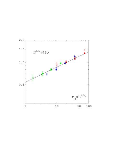
Figure 8: Logarithmic plot of Fig. 7. The QCD data of JLQCD (empty symbols) and Bielefeld (filled symbols) are compared to the asymptotic $O(4)$-finite-size-scaling function (solid line). The notation for the symbols is as in Fig. 7.

On the other hand the value of ${\langle\bar{\psi}\psi\rangle}$ at very small $m_{q}$ is more sensitive to the exact position of evaluation, because ${\langle\bar{\psi}\psi\rangle}$ is steeper there. Moreover, we are not precisely on a line of fixed $z$ and there is an additional finite-size effect due to the separate position determination at each point and for each lattice size. The error in the position location has not been taken into account in the plots. With increasing quark mass the data points in Fig. 8 must follow a straight line with slope $1/\delta$, if the universality hypothesis [1]-[3] is true. We have therefore compared the data to a line $\bar{c}+(1/\delta)\ln(m_{q}aL^{1/\nu_{c}})$, which represents the asymptotic finite-size-scaling function. Because of the unknown metric factors of QCD the constant $\bar{c}$ was chosen freely. We see in this comparison that the data are indeed compatible with the expected behaviour, especially when we take into account that the lattice sizes are still small and corrections are probably present. We have repeated the analysis with $O(2)$ exponents. They differ only slightly from the ones of $O(4)$: $\beta/\nu$ by 1.4%, $\nu_{c}$ by 0.3% and $\delta$ by 1.7%. The result is very similar to $O(4)$ and because of the spread of the data, one cannot really distinguish the two cases.

4 Summary and Conclusions

We have investigated finite-size-scaling (FSS) functions for the three-dimensional $O(4)$ and $O(2)$ spin models. Our aim was to provide a more suitable basis for a test of QCD lattice data on the conjectured universality class. In order to reduce the number of variables on which these FSS functions depend, we have calculated these functions along lines of fixed $z=th^{-1/\beta\delta}$ in the $(t,h)$-plane. This choice was motivated by two prominent examples of such lines: the critical line with $z=0$ and the pseudocritical line of peaks of the susceptibility. Simulations of QCD are usually performed in the neighbourhood of that line. In the $O(N)$ models we found the pseudocritical line from the known universal scaling functions for $V\rightarrow\infty$. The result was confirmed by a search with finite volume calculations.

On the critical line we found almost no corrections to scaling for $O(4)$, while for $O(2)$ strong ones appear, as would be expected. For both models the universal FSS functions are approached from below with increasing volume. On the pseudocritical line there are considerable corrections to scaling for both models. Here the approach to the universal FSS functions is from above. In both models and on both lines the asymptotic forms of the FSS functions are reached already at small values around 10 to 30 of the scaling variable $HL^{1/\nu_{c}}$ from below.

We have made FSS plots from two sets of $N_{f}=2$ QCD lattice data for ${\langle\bar{\psi}\psi\rangle}$ at the peak positions of the susceptibility $\chi_{m}$. The general behaviour of the data is similar to that of the $O(N)$ models from finite volumes. We find an approach to a limiting function from above, though at small quark masses (that is at small magnetic fields) the QCD data seem to be too high. The slope in the logarithmic plot of the data is nevertheless in nice agreement with the expectation $1/\delta$ of the $O(N)$ models. A test on the critical line would be even more preferable, because there the $t$ value is independent of $h$. The exact critical point of QCD is however difficult to determine and up to now unknown.

Acknowledgements

We owe special thanks to Kazuyuki Kanaya for sending us his complete chiral condensate data and to Edwin Laermann for helpful discussions and his QCD data on the pseudocritical line. We are grateful to David Miller for a careful reading of the manuscript. Our work was supported by the Deutsche Forschungsgemeinschaft under Grant No. Ka 1198/4-1, the work of T.M. in addition by FAPESP, Brazil (Project No.00/05047-5).

References

- [1] R. Pisarski and F. Wilczek, Phys. Rev. D29 (1984) 338.
- [2] F. Wilczek, J. Mod. Phys. A7 (1992) 3911.
- [3] K. Rajagopal and F. Wilczek, Nucl. Phys. B399 (1993) 395.
-
[4]
F. Karsch, Phys. Rev. D49 (1993) 3791;
F. Karsch and E. Laermann, Phys. Rev. D50 (1994) 6954. - [5] E. Laermann, Nucl. Phys. B (Proc. Suppl.) 63A-C (1998) 114.
- [6] S. Ejiri, Nucl. Phys. B (Proc. Suppl.) 94 (2001) 19.
- [7] D. Toussaint, Phys. Rev. D55 (1997) 362.
- [8] J. Engels and T. Mendes, Nucl. Phys. B572 (2000) 289.
- [9] Y. Iwasaki, K. Kanaya, S. Kaya and T. Yoshié, Phys. Rev. Lett. 78 (1997) 179.
- [10] A. Ali Khan et al. (CP-PACS Collaboration), Nucl. Phys. B (Proc. Suppl.) 83-84 (2000) 360 and Phys. Rev. D63 (2000) 034502.
- [11] J. Engels, S. Holtmann, T. Mendes and T. Schulze, Phys. Lett. B492 (2000) 219.
- [12] S. Aoki et al. (JLQCD Collaboration), Phys. Rev. D57 (1998) 3910.
- [13] E. Laermann, Nucl. Phys. B (Proc. Suppl.) 60A (1998) 180.
- [14] C. Bernard et al. (MILC Collaboration), Phys. Rev. D61 (2000) 054503.
- [15] A. Berera, Phys. Rev. D50 (1994) 6949.
- [16] R.B. Griffiths, Phys. Rev. 158 (1967) 176.
- [17] D.J. Wallace and R.K.P. Zia, Phys. Rev. B12 (1975) 5340.
- [18] C. Bagnuls and C. Bervillier, Phys. Rev. B41 (1990) 402 and Phys. Lett. A195 (1994) 163.
- [19] J. Engels, S. Holtmann, T. Mendes and T. Schulze, Nucl. Phys. B (Proc. Suppl.) 94 (2001) 861.
- [20] M. Hasenbusch and T. Török, J. Phys. A32 (1999) 6361.
- [21] K. Kanaya, private communication.
- [22] E. Laermann, private communication.