Chirality Correlation within Dirac Eigenvectors from Domain Wall Fermions

Abstract

In the dilute instanton gas model of the QCD vacuum, one expects a strong spatial correlation between chirality and the maxima of the Dirac eigenvectors with small eigenvalues. Following Horvath, et al. we examine this question using lattice gauge theory within the quenched approximation. We extend the work of those authors by using weaker coupling, $\beta=6.0$, larger lattices, $16^{4}$, and an improved fermion formulation, domain wall fermions. In contrast with this earlier work, we find a striking correlation between the magnitude of the chirality density, $|\psi^{\dagger}(x)\gamma^{5}\psi(x)|$, and the normal density, $\psi^{\dagger}(x)\psi(x)$, for the low-lying Dirac eigenvectors.

I Introduction

In a recent paper, Horvath, Isgur, McCune and Thacker [1] suggest that an important test of various theoretical models of the QCD vacuum can be made by examining the degree to which the space-time localization of a low-lying eigenmode of the Dirac operator is correlated with non-zero chirality. Such correlations are expected in the dilute instanton gas model of the QCD vacuum.

In this model, gauge configurations composed of widely separated instantons and anti-instantons support low-lying Dirac eigenvectors which are near superpositions of the zero modes that these (anti-)instantons would posses if in isolation. These near zero modes are proposed [2] to provide the non-zero density of Dirac eigenvalues, $\rho(\lambda)$ for vanishing eigenvalue $\lambda$, required by the Banks-Casher formula [3] and the non-zero QCD chiral condensate, $\pi\rho(0)=-12\langle\overline{q}q\rangle=(245{\rm MeV})^{3}$, where we give the value for $\langle\overline{q}q\rangle$ obtained in a recent quenched calculation [4] and the factor of 12 comes from our particular normalization conventions. Since the isolated zero modes associated with an (anti-)instanton are entirely (left-)right-handed, one should expect a strong correlation of handedness with the locations at which $\psi_{n}^{\dagger}\psi_{n}(x)$ is large.

Thus, this class of instanton-based models of the QCD vacuum can be tested by searching for such strong correlations between the chiral density $\psi_{n}^{\dagger}\gamma^{5}\psi_{n}(x)$ and normal density $\psi_{n}^{\dagger}\psi_{n}(x)$ for the low-lying eigenmodes of the Dirac operator on a configuration-by-configuration basis within a lattice QCD calculation. As emphasized by Horvath, et al. earlier arguments of Witten [5, 6] suggest that the large $N_{c}$ behavior of the $\eta^{\prime}$ mass may be inconsistent with the predictions of such an instanton model, providing additional motivation for such qualitative tests of the instanton picture.

In the above cited work of Horvath, et al., the authors search for such correlations using 30 gauge configurations obtained in the quenched approximation on a $12^{3}\times 24$ lattice volume with Wilson fermions and the Wilson gauge action with $\beta=5.7$. In this paper, we extend their study to smaller lattice spacing, $a^{-1}=1.922$ GeV, using a $16^{4}$ lattice volume which has a similar physical size of $\approx 1.6$ Fermi. Making use of configurations that we had already analyzed, we discuss here results from two different gauge actions. The first is the standard Wilson action with $\beta=6.0$ for which we have 32 configurations and the second uses the Iwasaki action with $\beta=2.6$, a value tuned to achieve the same lattice spacing. The latter ensemble contains 55 configurations.

Finally we employ an improved fermionic action, using the domain wall formalism of Shamir [7]. Further references to this method, our implementation of this lattice fermion action and a complete description of the notation used in this paper can be found in Ref. [4].

As is detailed below, using this finer lattice spacing and improved fermion formulation, we find a very different result from that seen in the earlier work of Horvath, et al. The chirality of the $n^{th}$ eigenmode, $|{\psi}_{n}^{\dagger}(x)\gamma^{5}\psi_{n}(x)|$ is surprisingly close to maximum at those lattice sites $x$ where the eigenmode is large. In Section II we briefly review the properties of the spectrum of the continuum Dirac operator and the closely related hermitian Dirac operator that we study. Section III explains the diagonalization procedure. In Section IV we present our results and analysis of the domain wall fermion eigenvectors. Finally, Section V contains a brief conclusion.

II Properties of the Continuum Dirac Operator

In the continuum, the Euclidean Dirac operator is usually written as a non-hermitian sum of an anti-hermitian operator $\mathchoice{\ooalign{$\hfil\displaystyle\mkern 1.0mu/\hfil$\crcr$\displaystyle D$}}{\ooalign{$\hfil\textstyle\mkern 1.0mu/\hfil$\crcr$\textstyle D$}}{\ooalign{$\hfil\scriptstyle\mkern 1.0mu/\hfil$\crcr$\scriptstyle D$}}{\ooalign{$\hfil\scriptscriptstyle\mkern 1.0mu/\hfil$\crcr$\scriptscriptstyle D$}}=\gamma^{\mu}D^{\mu}$ where $D^{\mu}$ is the usual gauge covariant derivative and a real mass term. The combined operator, $\mathchoice{\ooalign{$\hfil\displaystyle\mkern 1.0mu/\hfil$\crcr$\displaystyle D$}}{\ooalign{$\hfil\textstyle\mkern 1.0mu/\hfil$\crcr$\textstyle D$}}{\ooalign{$\hfil\scriptstyle\mkern 1.0mu/\hfil$\crcr$\scriptstyle D$}}{\ooalign{$\hfil\scriptscriptstyle\mkern 1.0mu/\hfil$\crcr$\scriptscriptstyle D$}}+m$, is easy to analyze being the sum of commuting hermitian and anti-hermitian pieces. However, the standard Wilson and domain wall lattice Dirac operators are more complex because the so-called Wilson mass term also contains derivatives causing the hermitian and anti-hermitian parts of these lattice Dirac operators to fail to commute. For the Wilson operator, $D_{W}$, this is easily remedied by working with the product $\gamma^{5}D_{W}$ which is readily seen to be hermitian. A similar construction is possible for domain wall fermions [8] where the product $\gamma_{5}R_{5}D$ is hermitian. Here $D$ is the domain wall Dirac operator, given for example in Eq. 1 of Ref. [4], and $R_{5}$ the reflection in the midplane in the fifth dimension, $s\rightarrow L_{s}-1-s$.

Our treatment differs from that of Horvath, et al. in that we work with the hermitian operator, finding real eigenvalues and their corresponding eigenvectors while the authors of Ref. [1] determine the complex eigenvalues of the non-hermitian Wilson operator and their corresponding eigenvectors. In order to compare our two results, we now review the relation between the eigenvectors of corresponding continuum operators: $\mathchoice{\ooalign{$\hfil\displaystyle\mkern 1.0mu/\hfil$\crcr$\displaystyle D$}}{\ooalign{$\hfil\textstyle\mkern 1.0mu/\hfil$\crcr$\textstyle D$}}{\ooalign{$\hfil\scriptstyle\mkern 1.0mu/\hfil$\crcr$\scriptstyle D$}}{\ooalign{$\hfil\scriptscriptstyle\mkern 1.0mu/\hfil$\crcr$\scriptscriptstyle D$}}+m$ and $\gamma^{5}(\mathchoice{\ooalign{$\hfil\displaystyle\mkern 1.0mu/\hfil$\crcr$\displaystyle D$}}{\ooalign{$\hfil\textstyle\mkern 1.0mu/\hfil$\crcr$\textstyle D$}}{\ooalign{$\hfil\scriptstyle\mkern 1.0mu/\hfil$\crcr$\scriptstyle D$}}{\ooalign{$\hfil\scriptscriptstyle\mkern 1.0mu/\hfil$\crcr$\scriptscriptstyle D$}}+m)$.

We begin by recalling the basic properties of the eigenmodes of the Dirac operator $\hfil\textstyle\mkern 1.0mu/\hfil$ $\textstyle D$ and the hermitian operator $\gamma^{5}\mathchoice{\ooalign{$\hfil\displaystyle\mkern 1.0mu/\hfil$\crcr$\displaystyle D$}}{\ooalign{$\hfil\textstyle\mkern 1.0mu/\hfil$\crcr$\textstyle D$}}{\ooalign{$\hfil\scriptstyle\mkern 1.0mu/\hfil$\crcr$\scriptstyle D$}}{\ooalign{$\hfil\scriptscriptstyle\mkern 1.0mu/\hfil$\crcr$\scriptscriptstyle D$}}$ in the continuum and then discuss properties of the local chiral density which is the focus of this paper. Since $\left\{\gamma^{5},\mathchoice{\ooalign{$\hfil\displaystyle\mkern 1.0mu/\hfil$\crcr$\displaystyle D$}}{\ooalign{$\hfil\textstyle\mkern 1.0mu/\hfil$\crcr$\textstyle D$}}{\ooalign{$\hfil\scriptstyle\mkern 1.0mu/\hfil$\crcr$\scriptstyle D$}}{\ooalign{$\hfil\scriptscriptstyle\mkern 1.0mu/\hfil$\crcr$\scriptscriptstyle D$}}\right\}=0$ and $\mathchoice{\ooalign{$\hfil\displaystyle\mkern 1.0mu/\hfil$\crcr$\displaystyle D$}}{\ooalign{$\hfil\textstyle\mkern 1.0mu/\hfil$\crcr$\textstyle D$}}{\ooalign{$\hfil\scriptstyle\mkern 1.0mu/\hfil$\crcr$\scriptstyle D$}}{\ooalign{$\hfil\scriptscriptstyle\mkern 1.0mu/\hfil$\crcr$\scriptscriptstyle D$}}^{\dagger}=-\mathchoice{\ooalign{$\hfil\displaystyle\mkern 1.0mu/\hfil$\crcr$\displaystyle D$}}{\ooalign{$\hfil\textstyle\mkern 1.0mu/\hfil$\crcr$\textstyle D$}}{\ooalign{$\hfil\scriptstyle\mkern 1.0mu/\hfil$\crcr$\scriptstyle D$}}{\ooalign{$\hfil\scriptscriptstyle\mkern 1.0mu/\hfil$\crcr$\scriptscriptstyle D$}}\,$, the spectrum of $\hfil\textstyle\mkern 1.0mu/\hfil$ $\textstyle D$ consists of pairs of eigenvectors $\psi_{\lambda}(x)$ and $\psi_{-\lambda}(x)=\gamma^{5}\psi_{\lambda}(x)$ with imaginary eigenvalues $\pm i\lambda$. For $\lambda=0$ the zero modes, $\{\psi_{0,i}\}_{1\leq i\leq N}$, can also be chosen eigenstates of $\gamma^{5}$, $\gamma^{5}\psi_{0,i}=\pm\psi_{0,i}$ since $\left[\gamma^{5},\mathchoice{\ooalign{$\hfil\displaystyle\mkern 1.0mu/\hfil$\crcr$\displaystyle D$}}{\ooalign{$\hfil\textstyle\mkern 1.0mu/\hfil$\crcr$\textstyle D$}}{\ooalign{$\hfil\scriptstyle\mkern 1.0mu/\hfil$\crcr$\scriptstyle D$}}{\ooalign{$\hfil\scriptscriptstyle\mkern 1.0mu/\hfil$\crcr$\scriptscriptstyle D$}}\right]\psi_{0,i}=0$. Here we have added the extra subscript $i$ to the zero modes to allow for the possibility that more than one eigenvector with zero eigenvalue exists. The Atiyah-Singer index theorem requires that the number of zero modes, $N$ satisfy, $N\geq|\nu|$ where $\nu$ is the integer winding number of the gauge field ($\nu=\dots-2,-1,0,1,2,\dots$).

Clearly, zero modes of $\hfil\textstyle\mkern 1.0mu/\hfil$ $\textstyle D$ are also zero modes of $\gamma^{5}\mathchoice{\ooalign{$\hfil\displaystyle\mkern 1.0mu/\hfil$\crcr$\displaystyle D$}}{\ooalign{$\hfil\textstyle\mkern 1.0mu/\hfil$\crcr$\textstyle D$}}{\ooalign{$\hfil\scriptstyle\mkern 1.0mu/\hfil$\crcr$\scriptstyle D$}}{\ooalign{$\hfil\scriptscriptstyle\mkern 1.0mu/\hfil$\crcr$\scriptscriptstyle D$}}$. The remaining eigenvectors of $\gamma^{5}(\mathchoice{\ooalign{$\hfil\displaystyle\mkern 1.0mu/\hfil$\crcr$\displaystyle D$}}{\ooalign{$\hfil\textstyle\mkern 1.0mu/\hfil$\crcr$\textstyle D$}}{\ooalign{$\hfil\scriptstyle\mkern 1.0mu/\hfil$\crcr$\scriptstyle D$}}{\ooalign{$\hfil\scriptscriptstyle\mkern 1.0mu/\hfil$\crcr$\scriptscriptstyle D$}}+m)$ can be easily related to those of $\mathchoice{\ooalign{$\hfil\displaystyle\mkern 1.0mu/\hfil$\crcr$\displaystyle D$}}{\ooalign{$\hfil\textstyle\mkern 1.0mu/\hfil$\crcr$\textstyle D$}}{\ooalign{$\hfil\scriptstyle\mkern 1.0mu/\hfil$\crcr$\scriptstyle D$}}{\ooalign{$\hfil\scriptscriptstyle\mkern 1.0mu/\hfil$\crcr$\scriptscriptstyle D$}}+m$ by diagonalizing the former on the two-dimensional subspace spanned by the basis $\left\{\psi_{\lambda},\psi_{-\lambda}\right\}$:

$$\gamma^{5}\left(\mathchoice{\ooalign{$\hfil\displaystyle\mkern 1.0mu/\hfil$\crcr$\displaystyle D$}}{\ooalign{$\hfil\textstyle\mkern 1.0mu/\hfil$\crcr$\textstyle D$}}{\ooalign{$\hfil\scriptstyle\mkern 1.0mu/\hfil$\crcr$\scriptstyle D$}}{\ooalign{$\hfil\scriptscriptstyle\mkern 1.0mu/\hfil$\crcr$\scriptscriptstyle D$}}+m\right)\left(\begin{array}[]{c}a\\ b\\ \end{array}\right) = \left(\begin{array}[]{cc}0&m-i\lambda\\ m+i\lambda&0\\ \end{array}\right)\left(\begin{array}[]{c}a\\ b\\ \end{array}\right)$$ (15)

$$= \lambda_{H}\left(\begin{array}[]{c}a\\ b\\ \end{array}\right).$$ (18)

The eigenvalues are easily seen to be

$$\lambda_{H}=\pm\left[\lambda^{2}+m^{2}\right]^{\frac{1}{2}}\,.$$ (19)

The normalized eigenvectors, $\psi_{H,\lambda_{H}}$ are

$$\psi_{H,\pm|\lambda_{H}|}=\frac{1}{\sqrt{2}\left(\lambda^{2}+m^{2}\right)^{\frac{1}{4}}}\left[\left(m-i\lambda\right)^{\frac{1}{2}}\psi_{\lambda}\pm\left(m+i\lambda\right)^{\frac{1}{2}}\psi_{-\lambda}\right]\,.$$ (20)

Next we compare the chiral density as determined by these two sets of eigenvectors. For zero modes:

$$\psi_{0,i}^{\dagger}(x)\gamma^{5}\psi_{0,i}(x)=\pm\psi_{0,i}^{\dagger}(x)\psi_{0,i}(x),$$ (21)

the largest value possible, for both the hermitian and non-hermitian operators. For the other, paired eigenvectors and the non-hermitian operator, the identity $\psi_{-\lambda}(x)=\gamma^{5}\psi_{\lambda}(x)$ implies that product

$$\psi_{\lambda}^{\dagger}(x)\gamma^{5}\psi_{\lambda}(x)=\psi_{-\lambda}^{\dagger}(x)\gamma^{5}\psi_{-\lambda}(x)=\chi(x)$$ (22)

is the same for each eigenvector $\psi_{\pm\lambda}$ in the pair. Similarly, the norm of the wave function at each point in space-time is the same for each pair of eigenvectors

$$\psi_{\lambda}^{\dagger}(x)\psi_{\lambda}(x)=\psi_{-\lambda}^{\dagger}(x)\psi_{-\lambda}(x)=\omega(x)$$ (23)

This is not true for the paired eigenvectors of the hermitian operator, where using Eq. 20 we find:

$$\psi_{H,\lambda_{H}}^{\dagger}(x)\psi_{H,\lambda_{H}}(x) = w(x)\pm\epsilon\chi(x)=\omega_{H}(x),$$ (24)

$$\psi_{H,\lambda_{H}}(x)\gamma^{5}\psi_{H,\lambda_{H}}(x) = \chi(x)\pm\epsilon\omega(x)=\chi_{H}(x),$$ (25)

where

$$\epsilon = \frac{m}{\sqrt{\lambda^{2}+m^{2}}}$$ (26)

and $\lambda=\pm|\lambda|$. In the chiral limit $\epsilon$ vanishes, and the local chiral densities of the anti-hermitian and hermitian Dirac operators coincide.

The above analysis should describe the properties of the low-lying eigenstates of the non-hermitian Wilson operator in the continuum limit. Thus, we conclude that the difference between the evaluation of the chiral density for the eigenvectors of the non-hermitian Wilson Dirac operator and those of the hermitian domain wall Dirac operator should agree in the continuum limit for those eigenvectors for which the parameter $\epsilon$ is small. Thus, the results presented in this paper and those of Horvath, et al. address the same continuum question and can be compared. Since in our calculation the explicit fermion mass is very small ($m_{f}=0$ for the Wilson action and $m_{f}=5\cdot 10^{-4}$ for the Iwasaki action) we expect that for most modes the parameter $\epsilon$ will also be very small making the normal and chiral densities the same for both operators. The only exception to this conclusion arises for the very smallest eigenvalues, $\lambda\approx 10^{-3}$ where $\epsilon$ may be of order one due to the residual mass coming from mixing between the walls, $m_{\rm res}\approx 10^{-3}$ for the Wilson action [4, 9] and $m_{\rm res}\approx 10^{-4}$ for the Iwasaki action [9, 10].)

III Diagonalization Method

Using the conjugate-gradient method proposed by Kalkreuter and Simma [11], we calculate the 19 lowest eigenvalues and eigenvectors of $D_{H}$. This corresponds to the range $0\mathrel{\hbox to0.0pt{\raise 2.20013pt\hbox{$<$}\hss}{\lower 2.20013pt\hbox{$\sim$}}}\lambda\mathrel{\hbox to0.0pt{\raise 2.20013pt\hbox{$<$}\hss}{\lower 2.20013pt\hbox{$\sim$}}}200$(MeV). In this section we describe our implementation of their method.

Following Kalkreuter and Simma, we use the conjugate gradient method to minimize the Ritz functional,

$$\mu(\Psi)={\langle\Psi|(D_{H})^{2}|\Psi\rangle\over\langle\Psi|\Psi\rangle}$$ (27)

on a sequence of subspaces orthogonal to the eigenvectors corresponding to the previously identified minima. When we have obtained our intended $N_{\rm max}=19$ eigenvectors, we then evaluate the $N_{\rm max}\times N_{\rm max}$ matrix $\langle\Psi_{k}|(D_{H})^{2}|\Psi_{j}\rangle$. This small matrix is then diagonalized by a Jacobi method and the resulting transformation used to improve the initial set of vectors $\{\Psi_{k}\}_{0\leq k<N_{\rm max}}$. This combination of conjugate gradient minimizations and small matrix diagonalizations is repeated until a sufficiently accurate result has been obtained.

This method requires the choice of two stopping criteria. For the sequence of $N_{\rm max}$ conjugate gradient minimizations of $\mu(\Psi_{k})$ we iterate each conjugate gradient procedure until the norm squared of the gradient of $\mu(\Psi_{k})$ with respect to $\Psi_{k}$ has decreased from its initial value by a factor of 10. This choice of $\gamma=0.1$, in the notation of Kalkreuter and Simma, was recommended by those authors and, after some testing, appeared to be a good choice for us. As a criterion to stop the outer iteration over $N_{\rm max}$ conjugate gradient minimizations followed by small matrix diagonalization, we required that the relative change in each of the eigenvalues be less than $10^{-7}$ after the final step in the method.

Since we are actually interested in the small eigenvalues and corresponding eigenvectors of $D_{H}$, we performed a follow-on step after the above procedure has yielded a best set of eigenvectors and eigenvalues of $D_{H}^{2}$. In this step, we used the Jacobi method again to diagonalize the $19\times 19$ matrix, $\langle\Psi_{k}|D_{H}|\Psi_{j}\rangle$ and the resulting transformation to rotate the original basis of 19 eigenvectors into what should be eigenvectors of $D_{H}$.

However, if the $19^{th}$ and $20^{th}$ eigenvalues of $D_{H}^{2}$ are nearly degenerate but the corresponding eigenvalues of $D_{H}$ have opposite signs, then this 19-dimensional subspace will in general not be invariant under the application of $D_{H}$. The $19^{th}$ eigenvector of $D_{H}^{2}$ can be an arbitrary mixture of the $19^{th}$ and $20^{th}$ eigenvectors of $D_{H}$. If this happens, we expect to see one “spurious” and 18 valid eigenvectors of $D_{H}$ after the Jacobi step. The spurious eigenvector will be orthogonal to the other 18 and the magnitude of the corresponding eigenvalue will be distributed arbitrarily between a correct $19^{th}$ value and zero.

One way to identify such a spurious eigenvalue is to look for an eigenvalue of $D_{H}$ whose square does not agree with any of the 19 eigenvalues of $D_{H}^{2}$. In practice we order the eigenvalues found for both $D_{H}$ and $D_{H}^{2}$ and consider 19 possible matches obtained by discarding one of the eigenvalues of $D_{H}$ and comparing the squares of the remaining 18 with the lowest 18 eigenvectors of $D_{H}^{2}$. The case with the largest sum of squares of relative differences identifies the spurious eigenvalue. This algorithm produces 18 “good” eigenvalues and discards the largest eigenvalue in the case that no spurious eigenvector is present. We use this method to determine the 18 eigenvectors analyzed in this paper.

A second method that in addition involves the eigenvector information evaluates the anti-commutator identity satisfied by $D_{H}$,

$$\{\Gamma_{5},D_{H}\}=2m_{f}Q^{\rm(w)}+2Q^{\rm(mp)},$$ (28)

where $Q^{\rm(w)}$ and $Q^{\rm(mp)}$ are pseudoscalar densities defined on the pairs of planes at $s=(0,L_{s}-1)$ and $s=(L_{s}/2-1,L_{s}/2)$, respectively, with precise definitions given in Ref. [4]. We compute the diagonal elements of this matrix equation in our basis of eigenvectors of $D_{H}$:

$$\Lambda_{n}\langle\Psi_{n}|\Gamma_{5}|\Psi_{n}\rangle=\langle\Psi_{n}|\Bigl{[}m_{f}Q^{\rm(w)}+Q^{\rm(mp)}\Bigr{]}|\Psi_{n}\rangle.$$ (29)

If for one or more eigenvectors the fractional difference of the left- and right-hand sides of Eq. 29 is larger than 0.12 we discard the eigenvector producing the largest difference. If all eigenvectors give differences lying below this value, we discard the largest eigenvalue. The fraction 0.12 is a somewhat arbitrary dividing point that separates the few large discrepancies from the majority with a much smaller difference.

Comparison of these two criteria shows disagreement on 4 of the 32 Wilson and 6 of the 55 Iwasaki configurations. However, in each of those cases one method discards the nineteenth eigenvalue while the other identifies either the seventeenth or eighteenth as spurious. Since the eigenvectors of these largest eigenvalues are likely the least well determined, we view this as satisfactory and expect that the difficulties from this imprecise identification of “spurious” eigenvectors enter our sample of eigenvectors on the level of a few percent or less.

IV Analysis and Results

In this section we examine some of the properties of the 18 lowest eigenvalues, $\Lambda_{H,i}$ and the corresponding eigenvectors $|\Lambda_{H,i}\rangle$ determined by the procedure described above,

$$D_{H}|\Lambda_{H,i}\rangle=\Lambda_{H,i}|\Lambda_{H,i}\rangle\quad(0\leq i<18).$$ (30)

The connection between these eigenvectors and eigenvalues and those of the usual 4-dimensional Dirac operator was discussed in detail in [4]. The 5-dimensional wave functions, $\Psi_{H,i}(x,s)$ are expected to represent the wave functions of 4-dimensional Dirac eigenfunctions with an added exponential dependence on the fifth coordinate $s$, causing $|\Psi_{H,i}(x,s)|^{2}$ to fall rapidly as $s$ moves away from the 4-dimensional planes $s=0$ and $s=L_{s}-1$, as shown, for example in Figs. 29 and 30 of Ref [4]. Likewise the eigenvalues $\Lambda_{H,i}$ should correspond to 4-dimensional Dirac eigenvalues.

For our conventions the components bound to the $s=0$ wall are predominately left-handed while those concentrated on the $s=L_{s}-1$ wall are right-handed. It is important to recall that for a lattice with finite $L_{s}$, a left-handed mode can propagate with a very small probability to the right-handed wall, and visa-versa, giving a small breaking of chiral symmetry which, for low energy phenomena, can be described by a residual quark mass, $m_{\rm res}$.

Our analysis is based primarily on 55 quenched gauge configurations generated with the Iwasaki gauge action [12] at $\beta=2.6$ and 4-dimensional lattice volume $16^{4}$. We also examine 32 configurations generated with the standard Wilson action at $\beta=6.0$ and the same volume. These two gauge actions have been choosen to correspond to approximately the same lattice spacing: $a^{-1}\approx 2$ GeV. The gauge configurations that we analyze are separated by 2000 sweeps of our updating algorithm, a simple two-subgroup heat-bath update of each link. The number of sites in the fifth dimension for the domain wall Dirac operator is $L_{s}=16$, and the domain wall height is $M_{5}=1.8$. For input quark mass we take $m_{f}=0$ for the Wilson action and $m_{f}=5\cdot 10^{-4}$ for the Iwasaki case. This small, non-zero value of $m_{f}$ is used in the Iwasaki case to avoid the very slow convergence of the Kalkreuter Simma method that we found when using $m_{f}=0$ for that action. Finally, the residual quark mass for these couplings is quite small, $m_{\rm res}\approx 0.0001$ for Iwasaki[9, 10], and $m_{\rm res}\approx 0.001$ for Wilson[9, 4] which correspond to 0.4 and 4 MeV, respectively.

To begin, let us examine the integrated or global chiral structure of $D_{H}$. We plot the magnitude of $\langle\Lambda_{H,i}|\Gamma^{5}|\Lambda_{H,j}\rangle$ in Figs. 1 and 2 for a typical “simple” and “complex” configuration. The matrix $\Gamma^{5}$ represents the physical $\gamma^{5}$ matrix in the domain wall fermion formalism [8]:

$$\langle\Lambda_{H,i}|\Gamma^{5}|\Lambda_{H,j}\rangle=\sum_{x\in V}\sum_{s=0}^{L_{s}-1}\Psi_{\Lambda_{H,i}}^{\dagger}(x,s){\rm sign}(s-(L_{s}-1)/2)\Psi_{\Lambda_{H,j}}(x,s)\,,$$ (31)

where $V$ is the 4-dimensional space-time volume.

The pattern seen in Fig. 1 for the simple configuration is precisely the chiral structure expected in the continuum. The single, diagonal element corresponding to $|\Lambda_{H,0}\rangle$ represents a zero mode which is an eigenstate of $\gamma^{5}$ with eigenvalue $+1$. (We will refer to such modes as “near zero modes” since for our choice of parameters, their eigenvalues are not precisely zero.) In our entire sample of Iwasaki and Wilson configurations, all such near zero modes have very small eigenvalues, $\Lambda\approx 10^{-3}-10^{-4}$, and all are either right-handed or left-handed within a given gauge configuration. Note this behavior is a natural consequence of the Atiyah-Singer theorem which requires an excess of right-handed to left-handed zero modes equal to the winding number of the background gauge configuration. This determines a minimum number of zero modes, all with the same chirality. The presence of additional zero modes would imply added constraints on the gauge background, corresponding to a set of zero measure if our near zero modes had a precisely zero eigenvalue. The remaining eigenvectors are grouped into pairs connected by $\gamma^{5}$ precisely as expected for the continuum Dirac operator in the limit of vanishing mass.

These simple continuum expectations are not satisfied by the complex configurations, such as that shown in Fig. 2. Of course, such configurations must be present for finite $L_{s}$ and finite lattice spacing. As the gauge configurations change continuously from one winding number to another, a plot of the sort shown in these figures must also change continuously and hence cannot always have the simple structure of Fig. 1. While for the Wilson gauge action somewhat more than half of the configurations show the complex pattern of Fig. 2, for the better-behaved Iwasaki case, this fraction has dropped to 10%. It should be emphasized that all the low-lying eigenvectors studied, both complex and simple ones, fall off rapidly away from the walls with the minimum magnitude of the wave function between the walls falling at least a factor thirty below its value on the two physical boundaries.

Such gauge configurations in which the winding number is changing can be associated with zero modes of the 4-dimensional Wilson Dirac operator with mass equal to $-M_{5}$ [13, 14]. Numerical simulations [15] suggest that the density of such 4-dimensional Dirac operator zero modes decreases exponentially with the exponential of the coupling, $\rho\sim e^{-c/\sqrt{a}}$, so that such effects may vanish rapidly as the continuum limit is approached.

Close to the continuum limit, the typical gauge configuration will be sufficiently continuous that its winding number can be identified [16]. As the winding number changes one expects that localized, rapidly changing gauge fields will appear and small dislocations, on the scale of a very few lattice spacings will appear or disappear. It is natural to speculate that such configurations produce the complex $\Gamma^{5}$ matrix elements of Fig. 2 and the non-zero density of 4-dimensional Dirac zero modes described above. The comparison of Iwasaki and Wilson results suggests that while such configurations are quite common for the Wilson gauge action when $a^{-1}\approx 2$ GeV, they are dramatically suppressed under similar circumstances by the form of the action proposed by Iwasaki. This general topic is the subject of much current research [17, 18, 19, 20].

If we are to systematically evaluate the domain wall fermion, QCD path integral, we must include all configurations in our analysis. Although we are explicitly examining the small eigenmodes of the Dirac operator, the eigenvalues and eigenfunctions represent a complex mixture of both long-distance and short-distance physics. While we are able to explicitly focus on small Dirac eigenvalues, the background gauge fields contain the full spectrum of short- and long-distance fluctuations. This is immediately demonstrated by the potential importance of small, very short-distance dislocations in the gauge configuration on quantities we are examining. However, we should also expect the more conventional short distance effects of wave function and mass renormalization, including short-distance contributions to the residual mass, to influence the low lying eigenvalues and eigenvectors analyzed here. A brief discussion of these effects on the eigenvalue spectrum can be found in Section VI C of Ref. [4]. We speculate that these complex configurations, which do not behave as is expected for smooth, continuum gauge fields, represent such short-distance effects. However, we should look carefully to see if configurations of the complex type introduce further chiral symmetry breaking at low energy beyond the simple residual mass described above. To date we have not recognized such effects.

The global chirality of our eigenvectors is summarized in Fig. 3. The distribution shows a large narrow peak around zero corresponding to the non-zero modes and two smaller, but also narrow, peaks at $\pm 1$ corresponding to near zero modes. From these figures it is clear that we can easily distinguish near zero modes from non-zero modes, except for the handful of outliers with chirality neither close to zero nor $\pm 1$.

Next we examine the distribution of local chirality, $X_{H}(x)/\Omega_{H}(x)$, which is shown in Figs. 4 and 5 for near zero modes and non-zero modes, respectively. Here the quantities $X_{H}(x)$ and $\Omega_{H}(x)$ are the generalizations of the continuum quantities $\chi_{H}(x)$ and $\omega_{H}(x)$ defined in Eq. 25, to the case of domain wall fermions:

$$\Omega_{H}(x) = \sum_{0\leq s<L_{s}}\Psi_{\Lambda_{H,i}}(x,s)^{\dagger}\Psi_{\Lambda_{H,i}}(x,s)$$ (32)

$$X_{H}(x) = \sum_{0\leq s<L_{s}}{\rm sign}(s-(L_{s}-1)/2)\Psi_{\Lambda_{H,i}}(x,s)^{\dagger}\Psi_{\Lambda_{H,i}}(x,s)$$ (33)

The six histograms superimposed in Figs. 4 and 5 correspond to histograms of the quantity $X_{H}(x)/\Omega_{H}(x)$ evaluated only at those sites where the normal density $\Omega_{H}(x)$ lies above a specified cut, for each of the eighteen eigenvectors that we have determined. The six cuts displayed correspond to the conditions: $\Omega_{H}(x)\cdot 10^{5}>3,4,5,6,7$ and 8 which include 8.6, 4.3, 2.4, 1.5 1.0 and 0.7% of the sites in the space-time lattice, respectively. These cuts correspond to sampling the local chirality, on average, from sites that account for 28, 19, 13, 10, 8, and 6%, respectively, of the total probability density of each eigenvector. In Table I we give these numbers with more precision for both the Iwasaki and Wilson cases.

The near zero mode distributions are sharply peaked at $\pm 1$ for all cuts, as expected. The non-zero mode distributions are also clearly double-peaked, with peaks centered approximately around $\pm.95\to\pm.8$, depending on the size of the cut. The distributions fill in between the peaks as more sites are sampled. Thus, our data show that definite chirality is strongly correlated with local maxima of both near zero and non-zero eigenmodes. The latter is certainly consistent with an instanton-dominated vacuum picture and is in disagreement with the recent work of Horvath, et al..

We also note that the strong correlation between chiral and normal density for our non-zero mode eigenvectors is also evident if we use the definition of local chirality in [1] instead of the ratio $X_{H}(x)/\Omega_{H}(x)$. In Fig. 6 we show a similar set of histograms for the Wilson gauge action. Clearly the same strong correlation between chiral and normal density is seen for this case as well.

We now discuss two important consistency checks on this potentially interesting result. First we determine the distribution of “global” chirality of each eigenvector when computed by including only those lattice sites selected by our cuts on $\Omega_{H}(x)$. We expect this distribution to be similar to that found when summing over all sites in the lattice, with each non-zero mode showing approximately zero total chirality. The results are shown in Fig. 7. While considerably broader than the distribution seen for the global chirality, it is still strongly peaked around zero with the sharpness of the peak decreasing as the cut on $\Omega_{H}(x)$ is made more stringent. This broadening is easily understood as the statistical effect of examining the sum over a smaller number of space-time points. Over-all, Fig. 7 is quite consistent with the expectation that chirality of the non-zero mode eigenvectors is quite evenly split between left- and right-handed lumps.

As a second consistency check, we investigate the extent to which the lowest lying 18 eigenmodes which we examine actually play an important role in the low energy physics described by the gauge configurations being studied. An easy way to address this question is to compute the contribution of the modes which we have isolated to the chiral condensate and to compare that contribution to the total chiral condensate determined independently [4]. In Table II and Fig. 8 we present such a comparison. As can be seen, these lowest 18 eigenvectors provide a large fraction of the actual value of $\langle\overline{q}q\rangle$ for the light input mass, $m_{f}=0$. For larger values of $m_{f}$, the contribution of these modes is a rapidly decreasing fraction of $\langle\overline{q}q\rangle$. However, for non-zero quark mass, the quadratically divergent contribution of high mass states $\propto m_{f}/a^{2}$ should make an increasingly important contribution. We can easily include these effects, by using a fit to $\langle\overline{q}q\rangle$ of the form

$$-\langle\overline{q}q\rangle=\frac{a_{-1}}{m_{f}+\delta m_{\langle\,\overline{q}\,q\,\rangle}}+a_{0}+a_{1}m_{f},$$ (34)

where $a_{-1}$, $a_{0}$, $a_{1}$ and $\delta m_{\langle\,\overline{q}\,q\,\rangle}$ are parameters determined and tabulated in Ref. [4]. The large coefficient $a_{1}$ describes these divergent contributions, allowing them to be included in our estimate of $\langle\overline{q}q\rangle$ by simply adding the term $a_{1}\cdot(m_{f}+m_{\rm res})$ to $-\langle\overline{q}q\rangle$. These results are included in Table II and Fig. 8. One sees that when this expected contribution from far off-shell states is included, we have good agreement with the directly computed values $\langle\overline{q}q\rangle$ for $m_{f}$ in the range between 0.0 and 0.01. This suggests that the 18 lowest modes that we have examined provide the bulk of the physical vacuum expectation value $\langle\overline{q}q\rangle$ and are therefore relevant to an attempt to characterize the physics of the QCD vacuum.

Finally, we note that the above results for the chiral density distribution of the near zero modes shown in Fig. 4 are not very illuminating since the local chirality is either left- or right-handed for all points in the lattice for these eigenvectors. A more informative picture is given in Fig. 9 which shows the magnitude of the right-handed components of a near zero mode in the $x-y$ plane summed over $z$ and $t$. The mode is clearly localized (and remains so in the other planes that are not shown). It is also dominantly right-handed since the left-handed component shown in Fig. 10 is more than 50 times smaller. These figures corresponds to the unique, near zero mode labeled as eigenvector 0 in Fig. 1.

For completeness, we include similar figures showing the spatial distribution of the right- (Fig 11) and left-handed (Fig. 12) parts of the first non-zero mode, numbered 1 in Fig. 1. These provide a particular illustration of the behavior shown in average terms in Fig. 5. The right-handed components of eigenvector 1 are centered around the point $(x,y,z,t)=(13,0,7,15)$ while the left-handed components of this eigenvector are largest at the distinct point $(11,9,3,6)$. This specific case shows a clear correlation between localization and chirality as would be expected in an instanton picture.

V Conclusion

We have examined the local correlation between the chirality and magnitude of the low-lying eigenmodes of the Dirac operator in quenched lattice QCD. A strong correlation is observed in our calculation suggesting a picture of the QCD vacuum containing background gauge fluctuations producing space-time regions in which the Dirac eigenstates are both localized and chiral. For those 0.7% of the lattice sites at which 6% of the eigenmode magnitude is concentrated, these eigenmodes are nearly eigenstates of $\gamma^{5}$ with $X_{H}(x)/\Omega_{H}(x)$ within 90% of 1. While this is certainly consistent with a vacuum described as a superposition of instantons, it is an important feature that may be accommodated by other models as well.

An essential ingredient of our calculation is the use of the domain wall fermion formulation. The domain wall Dirac operator readily identifies topological zero modes on gauge configurations as they appear in the Feynman path integral without resort to smoothing or cooling. The presence of these near zero modes in the domain wall Dirac spectrum is easily seen in the small mass behavior of the chiral condensate [21] and their implications for quenched calculations of the both the chiral condensate and hadron masses was discussed in detail in Ref. [4]. Related behavior has been found using the overlap Dirac operator [22, 23], an alternative lattice fermion formulation, also with improved chiral symmetry.

The recent calculation [1] using Wilson fermions which motivated this study found no chirality-localization correlation. However, the calculation of the present paper is improved over this earlier work in two significant respects. The most important is that we use domain wall fermions which preserve chiral symmetry to a high degree at non-zero lattice spacing [4, 9], while Wilson fermions do not. In addition the lattice spacing used here is roughly twice as small as that of Ref. [1].

Note added: After this paper was essentially complete, the recent work of DeGrand and Hasenfratz became available [24]. Our analysis and conclusions are quite similar to those of this paper. While both that paper and the present one, use improved fermion Dirac operators, overlap and domain wall respectively, we have used the gauge configurations directly, without smearing or fattening. This suggests that this strong correlation between spacial localization and chirality is seen even for gauge configurations whose fluctuations span the full range of distance scales produced by both the Iwasaki and Wilson gauge actions.

TABLE I.: Fractions of lattice sites and eigenvector normalization included for the six cuts, $\Omega_{H}(x)>\Omega_{\rm min}$, used in this paper.

	Iwasaki Action		Wilson Action
$\Omega_{\rm min}\cdot 10^{5}$	Fraction of	Fraction of	Fraction of	Fraction of
	lattice sites	normalization	lattice sites	normalization
3	0.086	0.285	0.080	0.319
4	0.043	0.186	0.042	0.235
5	0.024	0.132	0.026	0.186
6	0.015	0.100	0.017	0.156
7	0.010	0.079	0.012	0.136
8	0.007	0.064	0.009	0.121

TABLE II.: Contributions to the chiral condensate from the 18 lowest eigenvectors examined in this paper, $\langle\overline{q}q\rangle_{18}$, for five different quark mass values. In addition, we include the $\sim 1/a^{2}$ contribution from the large eigenmodes by including the term $a_{1}(m_{f}+m_{\rm res})$ using the values $a_{1}=3.97(8)10^{-4}$ and $m_{\rm res}=1.24(5)10^{-3}$ taken from Ref. [4]. Finally these results are compared with the complete value for $\langle\overline{q}q\rangle$ found in that paper. This comparison is done in the case of the Wilson action at $\beta=6.0$ where the detailed results for $\langle\overline{q}q\rangle$ are available from that earlier work.

$m_{f}$	$-\langle\overline{q}q\rangle_{18}$	$-\langle\overline{q}q\rangle_{18}+a_{1}(m_{f}+m_{\rm res})$	$-\langle\overline{q}q\rangle$
0.0	0.0036(6)	0.0037(6)	0.00219(20)
0.0025	0.00087(9)	0.00119(9)	-
0.005	0.00059(5)	0.00113(5)	0.00100(2)
0.0075	0.00048(3)	0.00124(3)	-
0.01	0.00043(2)	0.00140(2)	0.00134(1)

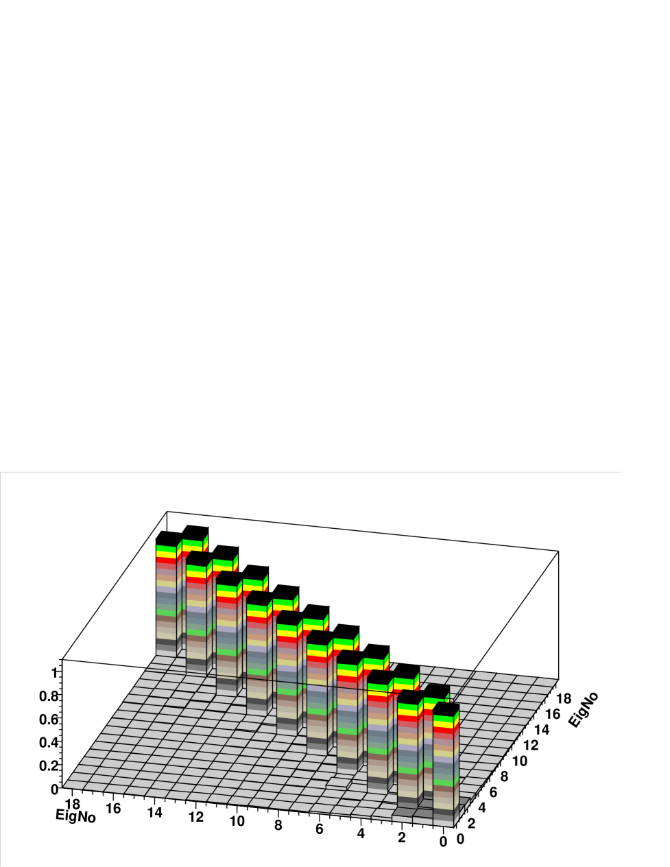
FIG. 1.: The magnitude of the matrix elements $\langle\Lambda_{H,i}|\Gamma^{5}|\Lambda_{H,j}\rangle$ evaluated on a “simple” configuration. The pattern seen is close to that expected for matrix elements of $\gamma^{5}$ in the continuum theory: The single near zero mode is an an approximate eigenstate of $\Gamma^{5}$ while the non-zero modes come in $\pm\Lambda_{H}$ pairs related by $\Gamma^{5}\Psi_{\Lambda_{H}}=-\Psi_{\Lambda_{H}}$.

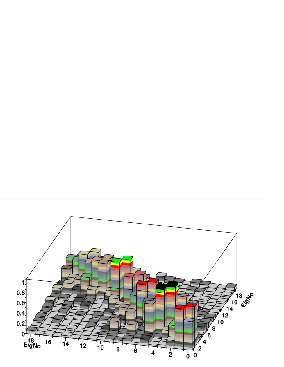
FIG. 2.: The magnitude of the matrix elements $\langle\Lambda_{H,i}|\Gamma^{5}|\Lambda_{H,j}\rangle$ evaluated on a “complex” configuration. For the Wilson gauge action more than one-half of the 32 configurations look like this while for the Iwasaki action only one in ten has this complex structure with the remaining 90% appearing similar to Fig. 1.

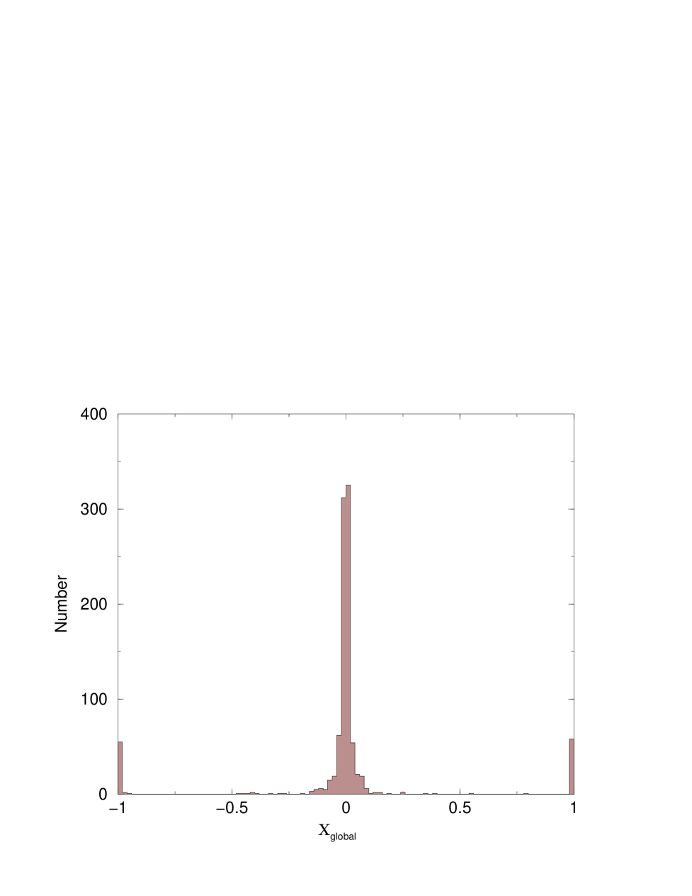
FIG. 3.: The distribution of global chirality of the eigenvectors of $D_{H}$ evaluated at zero input quark mass, $m_{f}=0$.

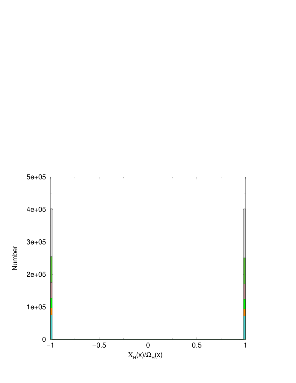
FIG. 4.: The distribution of local chirality $X_{H}(x)/\Omega_{H}(x)$ of near zero mode eigenvectors of $D_{H}$ on the Iwasaki ensemble of gauge fields for sites where $\Psi^{\dagger}(x)\Psi(x)$ is greater than an arbitrary imposed cut. The different cuts correspond to keeping between 1 and 8% of the total sites in the space-time lattice.

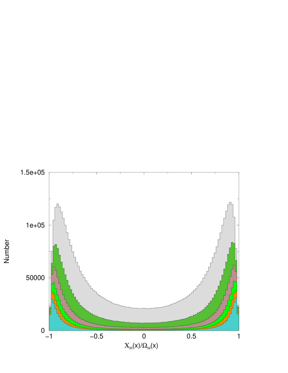
FIG. 5.: The same quantities as in Fig. 4, but for non-zero mode eigenvectors and again for the Iwasaki action. The double-peak structure is a feature expected in instanton-dominated models of the QCD vacuum.

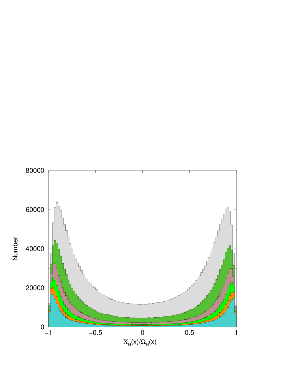
FIG. 6.: The same quantities as in Fig. 5, except now the Wilson gauge configurations are examined. The double-peak structure is very similar to that found in the Iwasaki case.

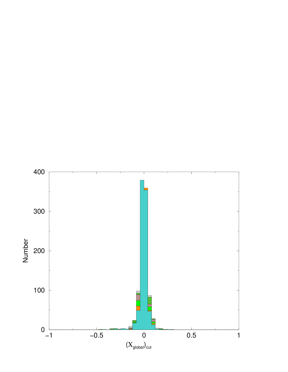
FIG. 7.: The distribution of chiral density for non-zero mode eigenvectors of $D_{H}$ summed over those lattice sites obeying the cuts imposed on $\Omega_{H}(x)$ as described in the text. As the cut is increased, the width of the distribution becomes more narrow. The distributions indicate that on average, chirality for a single eigenvector is evenly split into left- and right-handed lumps.

FIG. 8.: $\langle\overline{q}q\rangle$ for quenched simulations done on $16^{3}\times 32$ lattices at $\beta=6.0$ for $L_{s}=16$. In addition to the direct results for $\langle\overline{q}q\rangle$ presented in Ref. [4], and the fit of the form given in Eq. 34, we also plot the values obtained from the 18 eigenvectors studied here (filled triangles) and the sum of those values with the contribution from far off-shell states, $a_{1}(m_{f}+m_{\rm res})$ (filled diamonds).

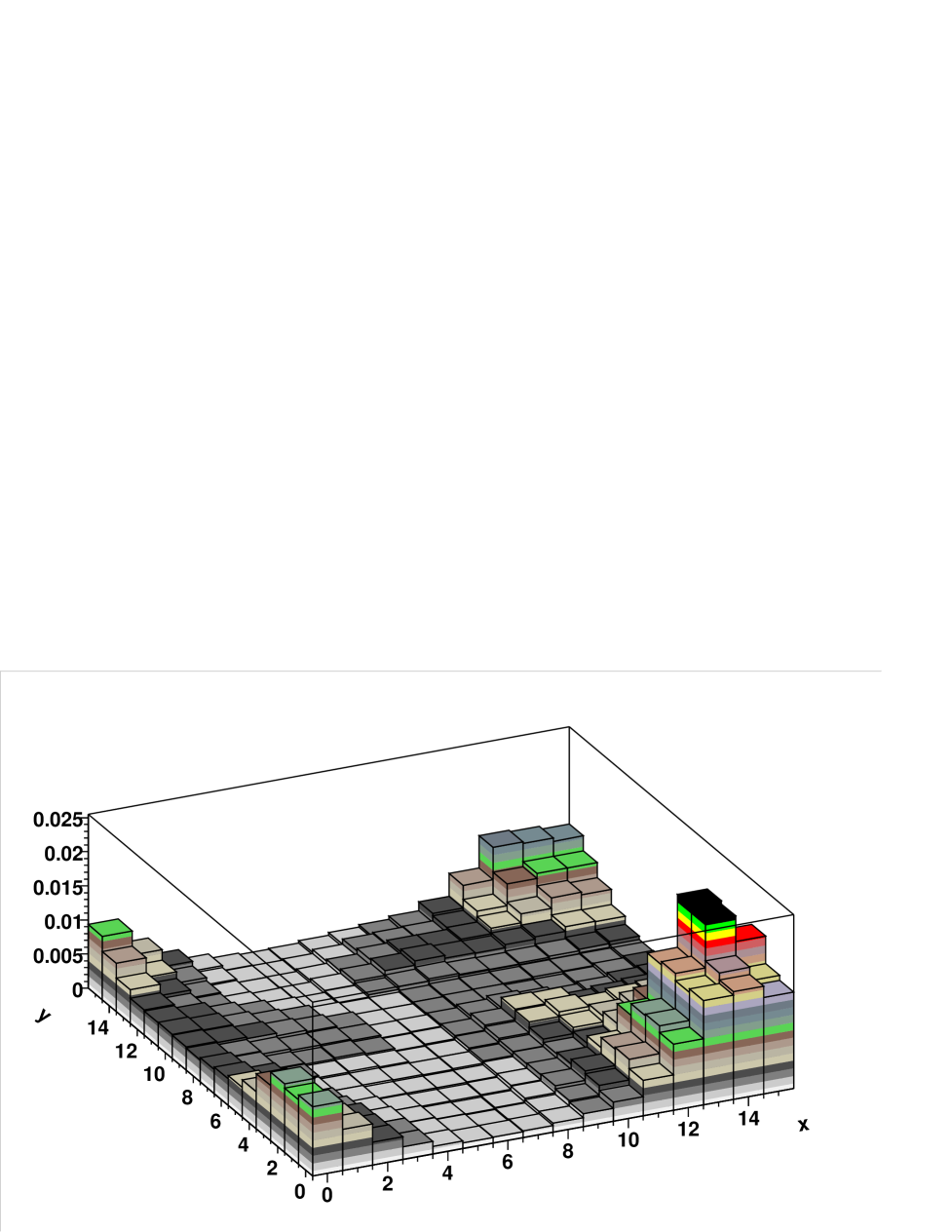
FIG. 9.: The distribution of the magnitude of the right-handed components of a near zero mode eigenvector of $D_{H}$ in the $x-y$ plane, summed over the $z$ and $t$ coordinates. A single, well-localized peak is visible near $x=14$ and $y=2-3$.

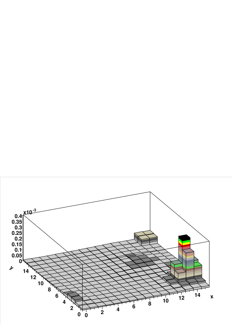
FIG. 10.: The distribution of the magnitude of the left-handed components of a near zero mode eigenvector of $D_{H}$ in the $x-y$ plane, summed over the $z$ and $t$ coordinates. This is the same eigenvector whose right-handed components are show in Fig. 9. While a peak can also be seen in this figure, its magnitude is 50 times smaller than that shown for the right-handed components.

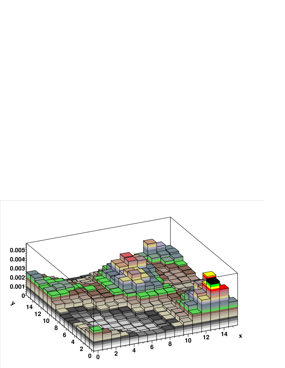
FIG. 11.: The distribution of the magnitude of the right-handed components of a non-zero eigenvector of $D_{H}$ in the $x-y$ plane, summed over the $z$ and $t$ coordinates. A single somewhat broad peak is seen with $x=13$ and $y=0$ or 15. [Note: it should be remembered that our periodic boundary conditions imply that the points $y=0$ and $y=15$ are adjacent.]

FIG. 12.: The distribution of the left-handed components of the non-zero eigenvector shown in Fig. 11. Note this shows a quite different peak from that in the previous figure with $(x,y)=(11,11)$

REFERENCES

- [1] I. Horvath, N. Isgur, J. McCune, and H. B. Thacker (2001), eprint hep-lat/0102003.
- [2] T. Schafer and E. V. Shuryak, Rev. Mod. Phys. 70, 323 (1998), eprint hep-ph/9610451.
- [3] T. Banks and A. Casher, Nucl. Phys. B169, 103 (1980).
- [4] T. Blum et al. (2000), eprint hep-lat/0007038.
- [5] E. Witten, Nucl. Phys. B149, 285 (1979).
- [6] E. Witten, Nucl. Phys. B156, 269 (1979).
- [7] Y. Shamir, Nucl. Phys. B406, 90 (1993), eprint hep-lat/9303005.
- [8] V. Furman and Y. Shamir, Nucl. Phys. B439, 54 (1995), eprint hep-lat/9405004.
- [9] A. A. Khan et al. (CP-PACS) (2000), eprint hep-lat/0007014.
- [10] We (RBC collaboration) have repeated the calculation of in [9] for and and find the same result .
- [11] T. Kalkreuter and H. Simma, Comput. Phys. Commun. 93, 33 (1996), eprint hep-lat/9507023.
- [12] Y. Iwasaki UTHEP-118.
- [13] R. Narayanan and H. Neuberger, Nucl. Phys. B443, 305 (1995), eprint hep-th/9411108.
- [14] R. G. Edwards, U. M. Heller, and R. Narayanan, Nucl. Phys. B535, 403 (1998), eprint hep-lat/9802016.
- [15] R. G. Edwards, U. M. Heller, and R. Narayanan, Phys. Rev. D60, 034502 (1999), eprint hep-lat/9901015.
- [16] M. Luscher, Commun. Math. Phys. 85, 39 (1982).
- [17] F. Berruto, R. Narayanan, and H. Neuberger, Phys. Lett. B489, 243 (2000), eprint hep-lat/0006030.
- [18] R. G. Edwards and U. M. Heller (2000), eprint hep-lat/0005002.
- [19] P. Hernandez, K. Jansen, and M. Luscher (2000), eprint hep-lat/0007015.
- [20] Y. Shamir, Phys. Rev. D62, 054513 (2000), eprint hep-lat/0003024.
- [21] G. T. Fleming et al., Nucl. Phys. Proc. Suppl. 73, 207 (1999), eprint hep-lat/9811013.
- [22] S. J. Dong, F. X. Lee, K. F. Liu, and J. B. Zhang, Phys. Rev. Lett. 85, 5051 (2000), eprint hep-lat/0006004.
- [23] T. DeGrand and A. Hasenfratz (2000), eprint hep-lat/0012021.
- [24] T. DeGrand and A. Hasenfratz (2001), eprint hep-lat/0103002.
- [25] D. Chen et al., Nucl. Phys. Proc. Suppl. 73, 898 (1999), eprint hep-lat/9810004.
- [26] R. D. Mawhinney, Parallel Comput. 25, 1281 (1999), eprint hep-lat/0001033.