The Ising Model on a Dynamically Triangulated Disk with a Boundary Magnetic Field

Abstract

We use Monte Carlo simulations to study a dynamically triangulated disk with Ising spins on the vertices and a boundary magnetic field. For the case of zero magnetic field we show that the model possesses three phases. For one of these the boundary length grows linearly with disk area, while the other two phases are characterized by a boundary whose size is on the order of the cut-off. A line of continuous magnetic transitions separates the two small boundary phases. We determine the critical exponents of the continuous magnetic phase transition and relate them to predictions from continuum 2-d quantum gravity. This line of continuous transitions appears to terminate on a line of discontinuous phase transitions dividing the small boundary phases from the large boundary phase. We examine the scaling of bulk magnetization and boundary magnetization as a function of boundary magnetic field in the vicinity of this tricritical point.

1 Introduction

The dynamical triangulations approach to (Euclidean) 2-d quantum gravity [1, 2, 3] arose from attempts to apply the Feynman path integral prescription for quantizing field theories to gravity. A straightforward application of the prescription would involve integrating over all 2-d manifolds of a given topology. For generic matter coupled systems this integration cannot be done. The dynamical triangulation method replaces the integral with a sum over discretized manifolds composed of identical equilateral triangles connected along their edges. In addition to including several exactly solvable models, the approach is also amenable to computer simulation using techniques from statistical physics. This is the approach we have taken in this paper.

Most work based on 2-d dynamical triangulations so far has been restricted to closed topologies where Liouville theory provides many predictions. The use of a topology with a boundary allows us to probe less well understood areas — in this case the Ising model coupled to a boundary magnetic field ($H$) and 2-d quantum gravity. This has been studied analytically [4, 5, 6]. The boundary magnetic field can be seen as interpolating between the only two conformally invariant boundary conditions: fixed ($H=\pm\infty$) and free ($H=0$). Away from these special boundary conditions, the model possesses the interesting property of being conformally invariant in the bulk, but not at the boundary. We describe our model in more detail in Section 2.

In principle, the model has four couplings. In the gravitational sector, there are couplings to the disk area (number of triangles,$A$) and to the boundary length ($l$). In the matter sector, there are the Ising coupling ($J$) and the boundary magnetic field. We describe our methods for simulating the model in Section 3. They were initially tested against a strong coupling expansion of the partition function. This along with measurements of the disk amplitude for zero Ising coupling are discussed in Section 4. Both agree with predictions.

For fixed disk area and zero boundary magnetic field, we have mapped the resultant 2-d phase diagram. We show evidence for three phases and associated critical lines, and use finite size scaling to extract estimates for critical exponents. These lines of transitions appear to meet at a unique tricritical point at which the system exhibits long range spin correlations and a non-trivial scaling of boundary length with disk area. This is presented in Section 5.

As explained in Section 6, we have tracked this tricritical point as a function of boundary magnetic field. We show our results concerning the scaling behavior of the model with non-zero boundary magnetic field and test some of the conjectures contained in [4]. Finally, we describe possible future work.

2 The Model

Our model consists of a 2-d triangulation composed of equilateral triangles connected along their edges with Ising [7] spins on the vertices. We allow only combinatorial triangulations; that is we exclude degenerate triangulations — no two triangles have the same three vertices, no triangle includes the same vertex twice and each triangle may have only one neighbor per edge. We characterize a configuration by its area, $A$, boundary length, $l$, and Ising spins, $\sigma_{i}$. The action for such a configuration is

$$S=-J\sum_{\left<ij\right>}\sigma_{i}\sigma_{j}-H\sum_{k\in\partial}\sigma_{k}+\mu A+\nu l$$ (1)

where $\left<ij\right>$ are nearest neighbor vertices, $\partial$ denotes the boundary of the disk, $J$ is the Ising coupling, and $\mu$ and $\nu$ are the cosmological constant and boundary cosmological constant respectively. The action contains no explicit gravitational component because, in two dimensions, the Gauss-Bonnet theorem implies that the Einstein-Hilbert action is a topological invariant [2]. The grand canonical partition function is

$$Z=\sum_{A,l}\sum_{t_{Al}}\sum_{\{\sigma_{i}\}}e^{-S}.$$ (2)

where $\sum_{t_{Al}}$ denotes a sum over all allowed triangulations of area $A$ and boundary length $l$.

3 Simulation Methods

A disk can be created from a sphere by simply cutting out a hole, and this observation forms the basis of our simulation method. If we consider a triangulated sphere with a single marked vertex and imagine cutting out this vertex and all the triangles containing it, we arrive at a triangulated disk. Furthermore every triangulated disk can be reached from an associated triangulated sphere. This allows us to sample the disk ensemble by sampling from a sphere ensemble using the usual procedures [8] — the only modification being that we identify one vertex as special, never allowing our local geometry changing moves to delete it. Additionally we do not endow it with an Ising spin. The special vertex along with the ring of triangles which contain it, form a cap which converts the disk into a sphere. Fig. 1 shows an illustration.

Figure 1: Making a disk from a sphere.

Our sampling of triangulations and Ising states is done with a Metropolis procedure [9]. Several types of moves are used in the simulation. For changes to the geometry, the moves are link flips, vertex insertions and vertex deletions. For changes to the Ising matter, we use either a local spin flip, or a Wolff cluster algorithm [10].

3.1 Geometry Moves

To change the geometry, we choose a triangle at random, then choose at random one of three types of geometry changing moves: link flips, vertex insertions, and vertex deletions. For vertex insertions, this completely specifies the move. For vertex deletions, we need to choose which of the chosen triangle’s three vertices to delete, while for link flips, we need to choose which of its three links to flip. Only vertices other than the special marked vertex and with exactly three surrounding triangles are allowed to be deleted. Notice that when a new vertex is added we must also assign a new Ising spin. Moves are disallowed if they would lead to a degenerate triangulation.

These moves are ergodic in the space of triangulated spheres, and since every disk can be converted into a sphere, they are also ergodic in the space of triangulated disks. In addition to ergodicity, we require detailed balance. Let $t$ be a triangulation, $a$ the set of spins on $t$ unchanged in the move and $b$ the set of spins on $t$ which potentially change in the move. The requirement of detailed balance is

$$e^{-S(t,a,b)}T(t,a,b\rightarrow t^{\prime},a,b^{\prime})$$ (3)

$$=e^{S(t^{\prime},a,b^{\prime})}T(t^{\prime},a,b^{\prime}\rightarrow t,a,b)$$

where $S(t,a,b)$ is the action and $T(t,a,b\rightarrow t^{\prime},a,b^{\prime})$ is the transition probability. Each of our geometry changing updates requires the transition probabilities satisfy this criteria. We have used two types of geometry move in our simulations — a simple Metropolis move and a more efficient heat bath style update — which are described below.

3.1.1 Simple Metropolis Algorithm

In this method, any spins which will be changed by the move are chosen at random from a uniform probability distribution in advance. In that case we have $b^{\prime}$ so

$$T(t,a,b\rightarrow t^{\prime},a,b^{\prime})=P_{p}(t,a,b\rightarrow t^{\prime},a,b^{\prime})P_{a}(t,a,b\rightarrow t^{\prime},a,b^{\prime})$$ (4)

where $P_{p}$ is the probability of proposing the move and $P_{a}$ is the probability of accepting the move. This leads to the following update probabilities: We accept a proposed vertex insertion with probability

$$P_{a}^{i}(t,a,b\rightarrow t^{\prime},a,b^{\prime})=\frac{A(t)}{A(t^{\prime})}\mbox{min}\{e^{-S(t^{\prime},a,b^{\prime})+S(t,a,b)},1\}$$ (5)

where $A(t)$ is the number of triangles in $t$. A proposed vertex deletion is accepted with probability

$$P_{a}^{d}(t^{\prime},a,b^{\prime}\rightarrow t,a,b)=\frac{1}{2}\mbox{min}\{e^{+S(t^{\prime},a,b^{\prime})-S(t,a,b)},1\}$$ (6)

while link flips are accepted with probability

$$P_{a}^{f}(t,a,b\rightarrow t^{\prime},a,b^{\prime})=\mbox{min}\{e^{-S(t^{\prime},a,b^{\prime})+S(t,a,b)},1\}.$$ (7)

3.1.2 Heat Bath Algorithm

In the heat bath variation, insertions or deletions are accepted or rejected without regard to the state of the vertex’s spin. In the case of insertions, the vertex’s spin is chosen from a heat bath distribution after the move has been accepted. The probabilities in this scheme are:

$$P^{d}_{a}(t^{\prime},a,b^{\prime}\rightarrow t,a)=\frac{1}{1+e^{-\Delta S_{\uparrow}}+e^{-\Delta S_{\downarrow}}}$$ (8)

and

$$P^{i}_{a}(t,a\rightarrow t^{\prime},a,b^{\prime})=\frac{A(t)}{A(t^{\prime})}\frac{e^{-\Delta S_{\uparrow}}+e^{-\Delta S_{\downarrow}}}{1+e^{-\Delta S_{\uparrow}}+e^{-\Delta S_{\downarrow}}}$$ (9)

where $\Delta S_{\uparrow}$ is the change in the action if the involved spin was or will be chosen to be up, and $\Delta S_{\downarrow}$ if it was or will be chosen to be spin down. The spin of inserted vertices are chosen from:

$$P(b^{\prime})=\frac{e^{-S(t^{\prime},a,b^{\prime})}}{\sum_{b^{\prime\prime}}e^{-S(t^{\prime},a,b^{\prime\prime})}}.$$ (10)

3.2 Spin Updates via Local Spin Flips

The procedure for updating a single Ising spin is to choose one at random and flip it subject to a Metropolis test. The probability of accepting a flip is

$$P_{a}^{s}(\sigma\rightarrow-\sigma)=\mbox{min}\{e^{-(S(-\sigma)-S(\sigma))},1\}.$$ (11)

3.3 Spin Updates via the Wolff Algorithm

The Wolff cluster algorithm [10] is an efficient way of updating Ising (or Potts) spins. Specifically, it has been shown to be very efficient at combating the effects of critical slowing near phase transitions. The algorithm begins by selecting a vertex at random. The spin of this vertex is assigned as the first spin of a cluster. The cluster is grown by examining all the vertex’s neighbors and adding to the cluster any with the same spin as the initial vertex with probability $1-e^{-2J}$. The cluster is then grown further by following the same procedure with all of the newly added vertices. The procedure is iterated until no new vertices are added. Finally, all the spins in the cluster are reassigned to a (single) random value. The Wolff cluster algorithm satisfies detailed balance for the Ising model:

$$\frac{P_{p}^{w}(t,a,b\rightarrow t,a,b^{\prime})}{P_{p}^{w}(t,a,b^{\prime}\rightarrow t,a,b)}=\frac{e^{-S_{I}(t,a,b^{\prime})}}{e^{-S_{I}(t,a,b)}}$$ (12)

where $P_{p}^{w}$ is the probability of proposing a move (growing a given cluster) via the Wolff update. Since, unlike the Metropolis algorithm, all moves are accepted this is the same as the probability of performing the move. The cluster algorithm relies on the fact that the action contains only nearest neighbor bond couplings. At non-zero boundary field this is not the case and we have used a generalization of the algorithm which handles non-Ising like terms.

Consider an Ising model with such non-Ising like additions to the action:

$$S(t,a,b)=S_{I}(t,a,b)+S_{O}(t,a,b)$$ (13)

where $S_{I}$ is the Ising action and $S_{O}$ is the new term. Let $P_{p}(t,a,b\rightarrow t,a,b^{\prime})$ be the probability of proposing a transition from $(t,a,b)$ to $(t,a,b^{\prime})$ and $P_{a}(t,a,b\rightarrow t,a,b^{\prime})$ be the probability of accepting the proposal. Now we require

$$\frac{P_{p}(t,a,b\rightarrow t,a,b^{\prime})}{P_{p}(t,a,b^{\prime}\rightarrow t,a,b)}\,\frac{P_{a}(t,a,b\rightarrow t,a,b^{\prime})}{P_{a}(t,a,b^{\prime}\rightarrow t,a,b)}=\frac{e^{-S_{I}(t,a,b^{\prime})}}{e^{-S_{I}(t,a,b)}}\frac{e^{-S_{O}(t,a,b^{\prime})}}{e^{-S_{O}(t,a,b)}}.$$ (14)

If we ignore the non-Ising interaction and propose transitions as the Wolff algorithm prescribes we will have

$$P_{p}(t,a,b\rightarrow t,a,b^{\prime})=P^{w}_{p}(t,a,b\rightarrow t,a,b^{\prime}).$$ (15)

This in conjunction with 12 and 14 gives,

$$\frac{P_{a}(t,a,b\rightarrow t,a,b^{\prime})}{P_{a}(t,a,b^{\prime}\rightarrow t,a,b)}=\frac{e^{-S_{O}(t,a,b^{\prime})}}{e^{-S_{O}(t,a,b)}}.$$ (16)

We satisfy this with the choice

$$P_{a}(t,a,b\rightarrow t,a,b^{\prime})=\mbox{min}\{e^{-(S_{O}(t,a,b^{\prime})-S_{O}(t,a,b))},1\}.$$ (17)

Thus we modify the usual cluster update so as to subject the entire move to a Metropolis step dependent only on the non-Ising like terms in the action.

For present purposes, the non-Ising addition to the action is the interaction of the boundary spins with the boundary magnetic field:

$$S_{O}=-H\sum_{i\in\partial}\sigma_{i}.$$ (18)

3.4 Critical Tuning, Fixing Area and Boundary Length

We expect the disk amplitude for the fixed area and boundary ensemble to be of the form [11, 12, 6]

$$Z(l,A)=l^{a}e^{\nu_{c}l}A^{b}e^{\mu_{c}A}e^{-\frac{l^{2}}{A}}.$$ (19)

In the above, $\mu_{c}$ and $\nu_{c}$ are the critical values of the cosmological constants.

Given the simulation methods we have described, both area $A$ and boundary length $l$ will fluctuate. We can not prevent these fluctuations without sacrificing ergodicity. However, if we modify the action by adding a geometry fixing part

$$S_{f}(\lambda_{\nu},\lambda_{\mu},l_{0},A_{0})=\lambda_{\nu}(l-l_{0})^{2}+\lambda_{\mu}(A-A_{0})^{2}$$ (20)

we can force the simulation to remain in the vicinity of some target area $A_{0}$ and boundary length $l_{0}$. Notice that these modification terms vanish for disks with these target values and we can hope to recover the results of the fixed area/boundary length ensemble with $A=A_{0}$ and $l=l_{0}$ by merely sampling such target disks from our ensemble.

With the above addition, the simulation will visit states with weight

$$W(l,A) = e^{-S_{f}(\lambda_{\nu},\lambda_{\mu},l_{0},A_{0})}Z_{lA}$$

$$= l^{a}e^{(\nu_{c}-\nu)l-\lambda_{\nu}(l-l_{0})^{2}}A^{b}e^{(\mu_{c}-\mu)A-\lambda_{\mu}(A-A_{0})^{2}}e^{-\frac{l^{2}}{A}}$$

If we assume that the average values of $l$ and $A$ will occur approximately where they maximize $W$, we have

$$\left.\frac{\partial}{\partial A}W(A,l)\right|_{\left<l\right>,\left<A\right>} = 0$$ (22)

$$\left.\frac{\partial}{\partial l}W(A,l)\right|_{\left<l\right>,\left<A\right>} = 0$$ (23)

which we can solve to get

$$\mu_{c}=-\frac{\left<l\right>^{2}}{\left<A\right>^{2}}-\frac{b}{\left<A\right>}+\mu+2\lambda_{\mu}(\left<A\right>-A_{0})$$ (24)

and

$$\nu_{c}=-\frac{a}{\left<l\right>}+\nu+2\lambda_{\nu}(\left<l\right>-l_{0})-\frac{2\left<l\right>}{\left<A\right>}.$$ (25)

These equations allow us, as a by-product, to read off estimates for the critical couplings $\mu_{c}$ and $\nu_{c}$ by measuring the mean area $\left<A\right>$ and boundary length $\left<l\right>$ . Of course to do this, in general, we need the values of the exponents $a$ and $b$ — numbers that are not generally known (see Section 4.2 for a counter example). Notice, however, that the values of $a$ and $b$ are irrelevant in the thermodynamic limit ($A_{0},l_{0}\rightarrow\infty$) so long as $l_{0}\ll A_{0}$. This condition will be met close to the tricritical point where $l\sim\sqrt{A}$.

4 Disk Amplitude and Strong Coupling

We have tested our simulation methods in two ways. In the first, which is akin to the small coupling expansion, we measure the frequency of visits to small triangulations and compare the results to known values. In the second, we measure pure gravity disk amplitudes and compare estimates of the exponents for area and boundary length with known values.

4.1 Strong Coupling

We may recast the partition function in the following form

$$Z=\left(\omega_{1}e^{-\mu}+\omega_{2}e^{-2\mu}+\omega_{3}e^{-3\mu}\ldots\right)$$ (26)

where $\omega_{A}$ represents the weight associated with triangulations of area $A$ with all other variables summed over. For large $\mu$, only the smallest triangulations survive and the coefficients $\omega_{A}$ may be calculated explicitly. This is referred to as the strong coupling expansion. Computationally, we can achieve the same result by explicitly limiting the simulation to triangulations less than a certain area. Unlike the above, this procedure does not require large $\mu$.

We hand counted the number of distinct triangulations for disks with areas up to five. The counting is weighted by inverse symmetry factors, the calculations of which were the most difficult part of the counting. For the case of $\mu=\nu=0$ and no Ising spins, the number of times the simulation visits triangulations of a given area and boundary length should be proportional to this count. In Tab. 1 we compare our hand calculated counts to the observed number of visitations by the simulation. The data are normalized so that the values in the first row are one. The agreement was excellent and served as an important confirmation of the correctness of our code.

$A,l$	count	visits
$1,3$	$1.00$	$1.00\pm 0.00$
$2,4$	$1.50$	$1.50\pm 0.01$
$3,3$	$1.00$	$0.99\pm 0.01$
$3,5$	$3.00$	$2.99\pm 0.01$
$4,4$	$3.75$	$3.75\pm 0.03$
$4,6$	$7.00$	$6.96\pm 0.10$
$5,3$	$3.00$	$2.99\pm 0.01$
$5,5$	$12.60$	$12.60\pm 0.10$
$5,7$	$18.00$	$17.93\pm 0.20$

Table 1: Comparison of the number of distinct triangulations for a given area and boundary to the frequency of visitations by the simulation with no Ising spins.

We extended this calculation to triangles with Ising spins and possible boundary fields. The results, shown in Tabs. 2 and 3, were also excellent.

$A,l$	count	visits
$1,3$	$1.00$	$1.00\pm 0.00$
$2,4$	$3.03$	$3.03\pm 0.04$
$3,3$	$2.04$	$2.03\pm 0.04$
$3,5$	$12.27$	$12.24\pm 0.30$
$4,4$	$15.44$	$15.43\pm 0.30$
$4,6$	$57.89$	$57.78\pm 1.00$
$5,3$	$12.45$	$12.45\pm 0.30$
$5,5$	$104.94$	$104.73\pm 3.00$
$5,7$	$301.05$	$300.61\pm 5.00$

Table 2: Comparison of the number of distinct triangulations for a given area and boundary to the frequency of visitations by the simulation with Ising spins included with $J=0.1$ and $H=0$.

$A,l$	count	visits
$1,3$	$1.00$	$1.00\pm 0.00$
$2,4$	$5.29$	$5.30\pm 0.20$
$3,3$	$2.07$	$2.09\pm 0.10$
$3,5$	$37.38$	$37.44\pm 2.00$
$4,4$	$27.17$	$27.31\pm 1.00$
$4,6$	$308.57$	$309.93\pm 20.00$
$5,3$	$12.76$	$12.81\pm 1.00$
$5,5$	$320.80$	$321.67\pm 20.00$
$5,7$	$2808.60$	$2820.27\pm 100.00$

Table 3: Comparison of the number of distinct triangulations for a given area and boundary to the frequency of visitations by the simulation with Ising spins, a Boundary Magnetic Field with $J=0.1$ and $H=1$.

4.2 Disk Amplitude

If we eliminate the Ising spins and tune the cosmological constants to their critical values, we obtain the disk amplitude which is predicted to take the form [11, 12, 6]

$$Z(A,l)=l^{a}A^{b}e^{-\frac{l^{2}}{A}}.$$ (27)

The exponents $a$ and $b$ are predicted to be $-\frac{1}{2}$ and $-\frac{5}{2}$ respectively. We have attempted to measure these exponents from our simulations. The exponent $b$ can be found by measuring the fraction of bulk vertices which are 3-fold coordinated, while $a$ can be obtained by fitting the so-called ‘baby universe’ distribution.

4.2.1 Measuring the exponent $b$

Let $t_{1}$ be a triangulation os a disk of area $A-2$ and boundary length $l$. Let $t_{2}$ and $t_{3}$ be disks of area $A$ and boundary length $l$. Detailed balance tells us

$$W(t_{1})P(t_{1}\rightarrow t_{2})=W(t_{2})P(t_{2}\rightarrow t_{1})$$ (28)

where $W(t_{1})$ is the weight of state $t_{1}$ and $P(t_{1}\rightarrow t_{2})$ is the probability of a transition from $t_{1}$ to $t_{2}$. From this we get

$$W(t_{1})\sum_{t_{2}}P(t_{1}\rightarrow t_{2})=\sum_{t_{2}}W(t_{2})P(t_{2}\rightarrow t_{1}).$$ (29)

We can use this to write the partition function as

$$Z(A-2,l) = \sum_{t_{1}}W(t_{1})$$ (30)

$$= \sum_{t_{2}}W(t_{2})\sum_{t_{1}}\frac{P(t_{2}\rightarrow t_{1})}{\sum_{t_{3}}P(t_{1}\rightarrow t_{3})}.$$ (31)

Now consider the ratio

$$\frac{Z(A-2,l)}{Z(A,l)} = \left<\sum_{t_{1}}\frac{P(t_{2}\rightarrow t_{1})}{\sum_{t_{3}}P(t_{1}\rightarrow t_{3})}\right>_{W(t_{2})}.$$ (32)

Since we have eliminated the Ising spins, the action is $0$ for all states and the transition probabilities are $1$ for all possible moves. That being the case, the sums over transition probabilities just count the number of possible moves. The number of possible insertions is equal to the number of triangles into which a new vertex can be inserted:

$$\sum_{t_{3}}P(t_{1}\rightarrow t_{3})=A-2,$$ (33)

while the number of possible deletions is equal to the number of bulk vertices with exactly three surrounding triangles, $N_{3}$,:

$$\sum_{t_{1}}P(t_{2}\rightarrow t_{1})=N_{3}.$$ (34)

So,

$$\frac{Z(A-2,l)}{Z(A,l)}=\left<\frac{N_{3}}{A-2}\right>_{W(t_{2})}.$$ (35)

Given the expected form of $Z$,

$$\left<\frac{N_{3}}{A-2}\right>_{W(t_{2})} = \left(\frac{A-2}{A}\right)^{b}e^{-\frac{l^{2}}{A-2}+\frac{l^{2}}{A}}$$ (36)

$$\ln\left<\frac{N_{3}}{A-2}\right>_{W(t_{2})} = -\frac{2b}{A}+O\left(\frac{1}{A^{2}}\right)$$ (37)

We generated data with areas between 50 and 1600 to test this and found it was statistically consistent with $b=-2.5$. Because the above partition function is only correct for large volumes, the best results are obtained by excluding disks smaller than some cutoff from the fits. Of course, excluding too much data will harm the fits — however our data shows a robust plateau close to the predicted value. This can be seen in Fig. 2.

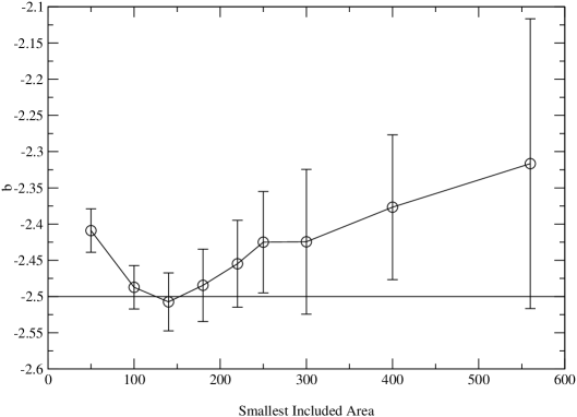
Figure 2: $b$ vs. smallest included volume.

4.2.2 Baby Universes and the exponent $a$

When two sections of the disk share a boundary of only one link, we say that the disk has split into two minimal neck baby universes. Using the form of the partition function mentioned above, the probability of a disk of area $A$ and boundary $l$ generating a baby universe of area $A_{1}$ and boundary $l_{1}$ is

$$P[A_{1},l_{1};A,l] = \frac{Z(A_{1},l_{1})Z(A-A_{1},l+2-l_{1})}{Z(A,l)}$$ (38)

$$= \left(\frac{l_{1}(l+2-l_{1})}{l}\right)^{a}\left(\frac{A_{1}(A-A_{1})}{A}\right)^{b}$$

$$\exp\{-\frac{l_{1}^{2}}{A_{1}^{2}}-\frac{(l+2-l_{1})^{2}}{(A-A_{1})^{2}}-\frac{l^{2}}{A^{2}}\}$$

We generated histograms of baby universe observations with various fixed disk areas and boundary lengths. To do this we found all such minimal necks on various equilibrium configurations and accumulated 2-d histograms labelled by the areas and boundary lengths of the smaller baby universes. Using the analytical value of $b=-2.5$, we found the value of $a$ which gave the best fit of the above probability distribution to the data. These are shown in Tab 4. The result for $A=2000$ is within $2\sigma$ of the predicted value $a=-\frac{1}{2}$ and we believe that the discrepancies for $A=1000$ and $A=500$ are likely finite size effects.

$A,l$	$a$	$\sigma$	$\chi_{\rm d.o.f.}^{2}$
500, 32	-0.451	0.0008	246.2
1000, 44	-0.487	0.001	41.0
2000, 64	-0.498	0.001	13.4

Table 4: $a$ which gives best fit to baby universe histogram.

5 Phase Diagram with $H=0$

For the work described in this section, both cosmological constants were set to their critical values. Areas were kept fixed, but $\lambda_{\nu}$ was set to zero, allowing the boundary length to fluctuate. We have identified phases based on two observables, magnetization and boundary length. To locate phase transitions we look for peaks in the corresponding susceptibilities. We define the magnetization of a given disk to be

$$M=\frac{1}{N}\left|\sum_{i}\sigma_{i}\right|$$ (40)

where $N$ is the number of vertices in the disk, and the sum is over all vertices. We use angle brackets to indicate averages over sampled disks, so $\left<M\right>$ refers to an average of $M$ over disks generated by the simulation. The magnetic susceptibility is

$$\chi_{M}=\frac{\partial\left<M\right>}{\partial J}=\left<NMM\right>-\left<NM\right>\left<M\right>.$$ (41)

When we refer to boundary susceptibility, we mean

$$\chi_{L}=\frac{\partial\left<L\right>}{\partial\nu}=\left<L^{2}\right>-\left<L\right>^{2}.$$ (42)

By these criteria we have found three phases — a paramagnetic phase with a small boundary (I), a ferromagnetic phase with a small boundary (II) and a paramagnetic phase with a large boundary (III). The locus of susceptibility peaks for $A=1000$ is shown in Fig. 3 and a schematic phase diagram is shown in Fig. 4

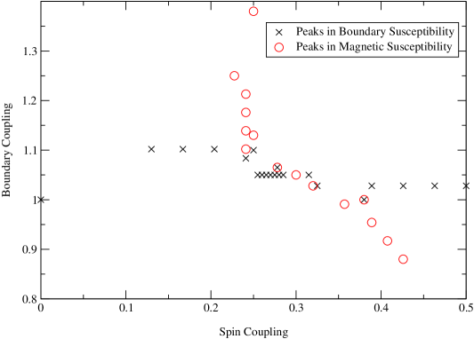
Figure 3: Observed peaks in susceptibilities for $A=1000$, $H=0$.

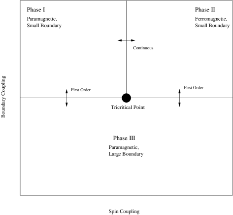
Figure 4: Schematic phase diagram at $H=0$.

We used finite size scaling to determine the order of the observed transitions. To make clear possible finite size effects, we looked at exponents for successive pairs of volumes. The scaling exponent for some quantity $x$ with values $x_{1}$ at area $A_{1}$ and $x_{2}$ at area $A_{2}$ is given by

$$\frac{\ln(x_{2}/x_{1})}{\ln(A_{2}/A_{1})}.$$ (43)

For sufficiently large boundary cosmological constant, $\nu$, the boundary length is minimal and we expect behavior similar to that of a marked sphere. In that case, there should be a continuous magnetic phase transition at $J_{c}=-\frac{1}{2}\ln\tanh\left(\frac{1}{2}\ln\frac{108}{23}\right)\approx 0.216273$. The observed magnetization and susceptibility in Fig.s 5 and 6 show this. Continuum calculations for 2-d quantum gravity coupled to $c=\frac{1}{3}$ matter predict $\left<NM^{2}\right>\sim A^{\frac{2}{3}}$ [13]. Tab. 5 shows values of this exponent extracted from data at succeeding pairs of areas. The agreement is quite good for the larger areas.

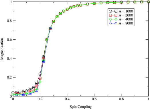
Figure 5: Magnetization, $\nu=5$, $H=0.$

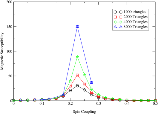
Figure 6: Magnetic susceptibility, $\nu=5$, $H=0$.

Areas	$\ln(x_{2}/x_{1})/\ln(A_{2}/A_{1})$
$1000-2000$	$0.70\pm 0.01$
$2000-4000$	$0.70\pm 0.01$
$4000-8000$	$0.69\pm 0.02$
$8000-16000$	$0.68\pm 0.02$
$16000-32000$	$0.67\pm 0.04$

Table 5: Scaling exponents of $x=\left<NM^{2}\right>$ at transition between phases I and II.

For sufficiently small $\nu$, the boundary length is maximal and, as shown in Fig. 7, the geometry is like that of a branched polymer. In this essentially 1-d configuration we expect that the system will not magnetize. However, from Fig.s 3 and 8, it appears that the line between Phases I and II continues into small $\nu$. Notice, though, that the susceptibility scaling exponents on this continuation, shown in Tab. 6, decrease as the disk area is increased. This indicates that the continuation is a finite size artifact. To confirm this we examined how the mean magnetization varies with area at $\nu=-5$ and $J=0.75$ which would be within this small-boundary, ferromagnetic phase if it existed. We fit the data to the form $c_{0}+c_{1}*A^{c_{2}}$ with the constraints $0<=c_{0},c_{1}<=1$. As shown in Fig. 9, extrapolation based on this fit implies that the magnetization will approach zero as the area is sent to infinity. To the extent that the fit does not agree with the data, the fit seems to be underestimating the rate of decrease so the predication appears safe. Our conclusion is that for small $\nu$ there is only one phase (III) characterized by a large boundary and unmagnetized spins.

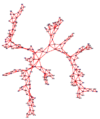
Figure 7: A triangulation, $J=5,\nu=-5$, $H=0$.

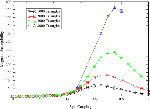
Figure 8: Magnetic susceptibility, $\nu=-5$, $H=0$.

Areas	$\ln(x_{2}/x_{1})/\ln(A_{2}/A_{1})$
$1000-2000$	$0.832\pm 0.006$
$2000-4000$	$0.765\pm 0.008$
$4000-8000$	$0.68\pm 0.01$
$8000-16000$	$0.60\pm 0.02$
$16000-32000$	$0.51\pm 0.04$

Table 6: Scaling exponents of $x=\left<NM^{2}\right>$ for $\nu=-5$ and $J=0.75$, $H=0$.

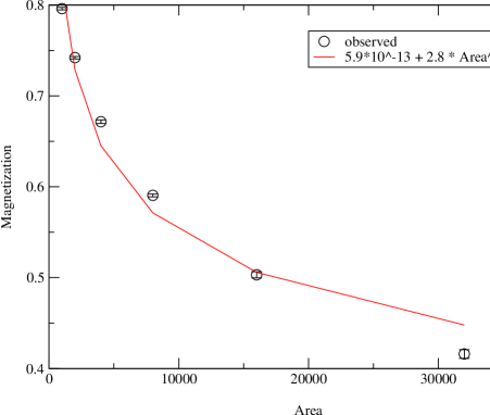
Figure 9: Magnetization vs. area, $J=0.75,\nu=-5$, $H=0$.

Fig. 10 and Tab. 7 show that along the transition from small (I,II) to large (III) boundary phases, the mean boundary length appears to jump discontinuously as $\nu$ is varied and the boundary length susceptibility exhibits a critical exponent of approximately one. This is strong evidence that the transition is first order.

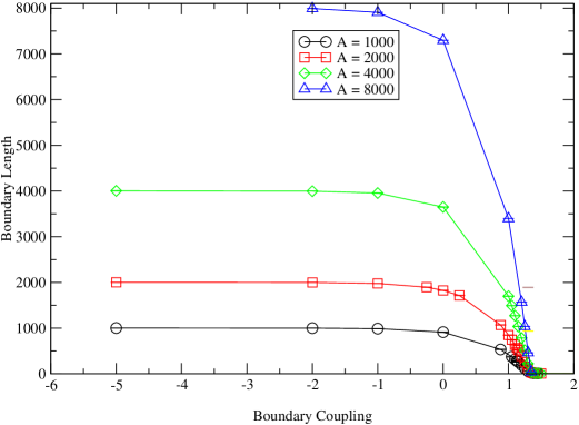
Figure 10: Boundary length, $J=1$, $H=0$.

Areas	$\ln(x_{2}/x_{1})/\ln(A_{2}/A_{1})$
$1000-2000$	$1.38\pm 0.01$
$2000-4000$	$1.07\pm 0.02$
$4000-8000$	$0.97\pm 0.02$
$8000-16000$	$0.99\pm 0.002$
$16000-32000$	$0.96\pm 0.02$

Table 7: Scaling exponent of $x=\left<l^{2}\right>-\left<l\right>^{2}$ for $J=1.0$, $\nu=1.3$ and $H=0$.

6 Scaling Behavior with a Boundary Field

At the tricritical point, we performed simulations to test the predictions of [4] regarding the scaling of the bulk magnetization, the boundary magnetization and their susceptibilities with the boundary magnetic field. For this part of the investigation, the Ising coupling was set to its continuum critical value. To reduce the number of parameters we needed to keep track of, the boundary lengths were fixed at $\sqrt{A}$. While this does involve tuning $\nu$ to its critical value, the boundary-length-fixing Gaussian in the action makes its exact value unimportant. Had we not done this, the approximate nature of the boundary coupling tuning procedure would have made comparing data from different runs more difficult.

The existence of a boundary magnetic field breaks the symmetry between up and down spins, so we no longer need to take the modulus of the spin sums. We can now define magnetizations

$$M_{\not\partial}=\frac{1}{N-l}\sum_{i\notin\partial}\sigma_{i}$$ (44)

$$M_{\partial}=\frac{1}{l}\sum_{i\in\partial}\sigma_{i}.$$ (45)

The susceptibilities are defined in the usual manner. Expressions for both boundary and bulk magnetizations are derived in [4]:

$$\left<M_{\partial}\right>=\frac{(e^{2H}-1)(3+(2+\sqrt{7})e^{2H})}{(1+(-1+\sqrt{7})e^{2H}+(2+\sqrt{7}e^{4H})}$$ (46)

and

$$\left<M_{\not\partial}\right>\sim L^{\frac{1}{3}}A^{-\frac{1}{3}}$$ (47)

where

$$L=\alpha(H)l$$ (48)

and

$$\alpha(H)=\frac{e^{2H}(1+e^{2H})}{1+(-1+\sqrt{7})e^{2H}+(2+\sqrt{7})e^{4H}}.$$ (49)

However, at least some of these results are dependent on the exact nature of the discretization procedure, i.e. the nature of the lattice ensemble. Our ensemble of so-called combinatorial triangulations is a subset of the set of triangulations employed by these authors. In concrete terms we might expect that the function $\alpha(H)$ relevant to a description of the combinatorial ensemble might differ substantially from the function given above. In spite of this it is reasonable to expect qualitatively similar behavior in the two cases. We have therefore looked for a boundary magnetization which increases with $H$ and is independent of $A$ and $l$, as well as a bulk magnetization which decreases with $H$ for fixed $l$. The boundary magnetization plot shown in Fig. 11 indeed illustrates this predicted behavior. In contrast, Fig. 12 shows the bulk magnetization increases with $H$.

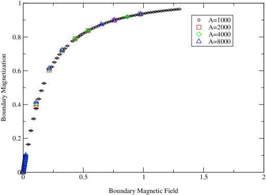
Figure 11: Boundary magnetization vs. boundary magnetic field at the tricritical point.

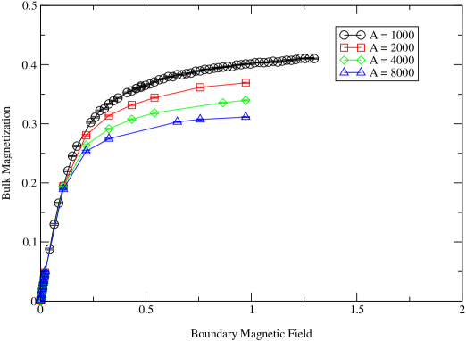
Figure 12: Bulk magnetization vs. boundary magnetic field at the tricritical point.

Caroll, Ortiz and Taylor speculate that their predicted decrease of bulk magnetization with $H$ is due to an increase in the average spin’s distance from the boundary when the boundary field is increased. To test this, we measured geodesic distances from all vertices on the disks to the boundary as follows. All boundary vertices are labelled as having a geodesic distance from the boundary of zero. All vertices connected to the boundary vertices and not already labelled are labelled as having a geodesic distance from the boundary of one. We continue labelling successively deeper vertices until there are none left. At that point we compute the average distance from the boundary. We observed behavior opposite that predicted by Caroll, Ortiz and Taylor: the mean distance to the boundary, illustrated in Fig. 13 decreases with increasing magnetic field. This behavior is then consistent with the behavior of the bulk magnetization.

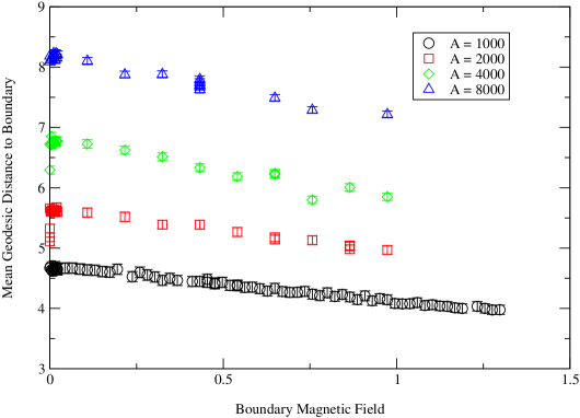
Figure 13: Mean geodesic distance from boundary vs. boundary magnetic field at the tricritical point.

An additional prediction is that the boundary magnetic susceptibility should be finite, $\chi_{\partial}=\frac{1+2\sqrt{7}}{3}$, in the limit of $H\rightarrow 0$ and $A\rightarrow\infty$. This differs markedly from the flat-space behavior of infinite susceptibility [14] which exhibits a logarithmic singularity. To compare this result with the numerical simulations we must be careful. The matrix model result is a prediction for the behavior of the boundary susceptibility on an infinite area disk as the boundary magnetic field is tuned to zero. Our simulations are carried out at finite area and so we should not take $H$ all the way to zero to do the comparison (the magnetic field effectively fails to break the symmetry of the Ising action for fields $H<1/l$). Thus we are led to examine the dependence of the susceptibility on the disk area for small but non-zero magnetic fields. In Tab. 8 we show finite size scaling exponents for the boundary magnetic susceptibility at three small boundary magnetic field strengths. While the exponents at $H=0.0216$ are positive, which would indicate a divergence, this field strength is below the value needed to break the spin-up, spin-down symmetry for the smallest disks of area $1000$ ($\frac{1}{\sqrt{1000}}\approx 0.0316$). For the larger values of $H$, we find negative exponents which imply a finite value of the susceptibility for small magnetic field in the infinite area limit. This is in qualitative agreement with the matrix model predictions and quite different from the flat space result.

$H$	$A1,A2$	$\frac{\log{\chi_{2}/\chi_{1}}}{\log{l_{2}/l_{1}}}$
0.0216	1000,2000	0.0863
	2000,4000	0.0891
	4000,8000	0.0651
0.108	1000,2000	-0.0190
	2000,4000	-0.0218
	4000,8000	-0.0197
0.216	1000,2000	-0.0490
	2000,4000	-0.0361
	4000,8000	-0.0636

Table 8: Critical exponent of boundary magnetic susceptibility at the tricritical point.

We have looked at the behavior of three geodesic correlation functions which measure the average properties of the spins as a function of distance to the boundary. The first of these, $n_{1}(r,N)$, measures the mean number of vertices encountered at distance $r$ from the boundary. The second, $n_{\sigma}(r;N)$, measures the net (integrated) magnetization and the third, $M(r;N)$, the mean magnetization at distance $r$ from the boundary. They are defined explicitly as follows

$$n_{1}(r;N)= \left<\sum_{i}\delta_{D_{i},r}\right> \sim N^{1-1/d_{H}}F_{1}(r/N^{1/d_{H}})$$ (50)

$$n_{\sigma}(r;N)= \left<\sum_{i}\sigma_{i}\delta_{D_{i},r}\right> \sim N^{1-\Delta-1/d_{H}}F_{\sigma}(r/N^{1/d_{H}})$$ (51)

$$M(r;N)= \left<\sum_{i}\frac{\sigma_{i}\delta_{D_{i},r}}{\sum_{k}\delta_{D_{k},r}}\right> \sim N^{-\Delta}g_{M}(r/N^{1/d_{H}})$$ (52)

where we have also introduced finite size scaling forms for these three functions analogous to the functions used for geodesic correlation functions defined on the sphere in [15]. Requiring that the area ($N\sim A$) dependence in $M(r;N)$ disappear for small $r$ implies that this correlation function takes on a simple power law form for small $x$

$$g_{M}(x)\sim x^{-d_{H}\Delta}$$ (53)

so that

$$M(r;N)\sim r^{-d_{H}\Delta}.$$ (54)

Figs. 14, 15, and 16 show our finite size scaling data for a representative value of $H=0.433$ and yield estimates for $1/d_{H}=0.27\pm 0.05$ and $\Delta=0.1\pm 0.02$.

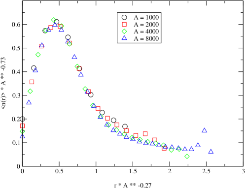
Figure 14: Number of vertices at geodesic distance $r$ from the boundary at the tricritical point with $H=0.433$.

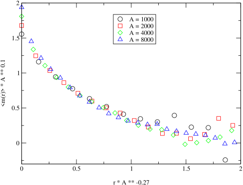
Figure 15: Magnetization of vertices at geodesic distance $r$ from the boundary at the tricritical point with $H=0.433$.

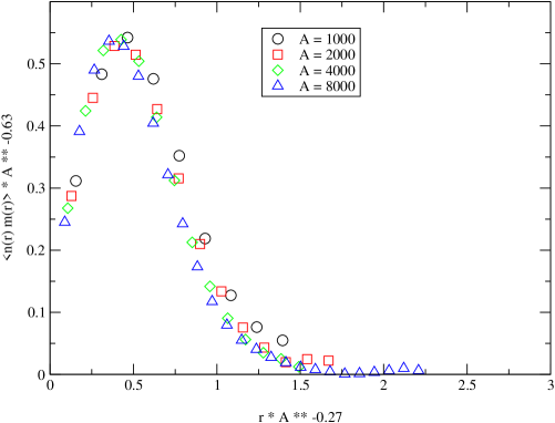
Figure 16: Sum of spins of vertices at geodesic distance $r$ from the boundary at the tricritical point with $H=0.433$.

The value for the fractal dimension, $d_{H}\approx 4$, is consistent with its value on the sphere and compatible with the idea that the fractal geometry of the disk far from the boundary is identical to the quantum geometry of the sphere and the expectation that the influence of the boundary decreases as one looks at spins further and further into the disk. This leads to the prediction that, in the continuum limit, the bulk quantities should exhibit KPZ [16] behavior.

Specifically, we have examined the scaling of the bulk magnetization and susceptibility at the tricritical point. Fig. 17 shows a plot of the logarithm of the susceptibility versus the logarithm of the area for a variety of boundary magnetic fields. The lines show good power law fits at a variety of $H$ with exponents ranging from 0.6 to 0.7 which is in approximate agreement with the KPZ prediction of $2/3$.

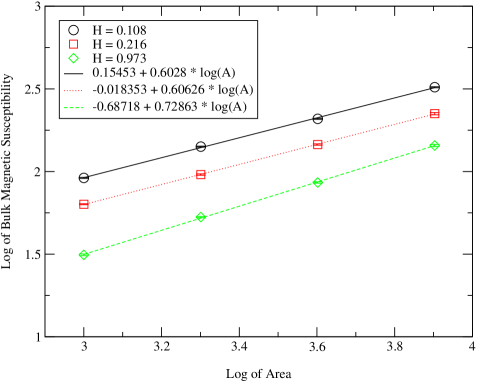
Figure 17: Scaling of bulk magnetic susceptibility with area for $H>0$ at the tricritical point.

The situation for the bulk magnetization is more complicated. We would expect that this would decrease with area according to the simple power law $\left<M_{\not\partial}\right>\sim A^{-\Delta}$ with $\Delta=\frac{1}{6}$ predicted by KPZ and consistent with Eq. 47 using $l=\sqrt{A}$. However, the finite size scaling result above as well as fits of the same data as used in Fig. 12 to powers of area yield exponents closer to $0.1$. This value differs quite markedly from the prediction. This may reflect a finite size effect involving the influence of spins close to the boundary where $d_{H}\approx 2$. It is interesting to observe that the resulting exponent for $M(r;N)$, $\Delta d_{H}\approx 0.37$ is near the value obtained in [4, 5] of $0.33$ using $\Delta=\frac{1}{6}$ and $d_{H}=2$. From Eqs. 47 and 48,

$$\left<M_{\not\partial}\right>A^{\frac{1}{6}}={\left[\alpha(H)\right]}^{-\frac{1}{3}}.$$ (55)

We hypothesize that the finite size effects can be taken into account by generalizing this to

$$\left<M_{\not\partial}\right>A^{b}=f(HA^{a}).$$ (56)

(Note that rescaling $H$ with $A$ is equivalent to rescaling it with $l$ since we have $l=\sqrt{(}A)$.) Assuming $a<0$ and expanding for large $A$,

$$\left<M_{\not\partial}\right>\approx f_{0}A^{-b}+f_{1}HA^{-b+a}+\frac{1}{2}f_{2}H^{2}A^{-b+2a}+...$$ (57)

Since we know that $\left<M_{\not\partial}\right>=0$ for zero $H$ we must have $f_{0}=0$. We found our data fit this well with $a=-0.067\pm 0.005$ and $b=0.1\pm 0.02$ (See Fig. 18). If our hypothesis is corect, then our data is consistent with

$$\left<M_{\not\partial}\right>\sim A^{-0.167}\approx A^{-\frac{1}{6}}$$ (58)

as predicted.

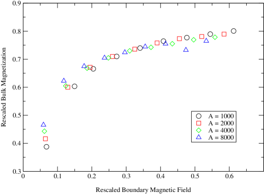
Figure 18: $\left<M_{\not\partial}\right>A^{0.1}$ vs. $HA^{-0.067}$ at the tricritical point.

To examine the scaling of the bulk magnetization further, we have calculated

$$\frac{\log\left(\frac{M(r;N)}{M(r+1;N)}\right)}{\log\left(\frac{r}{r+1}\right)}$$ (59)

which defines an effective (distance dependent) power law exponent for this correlation function. Fig. 19 shows these exponents for $r=1\mbox{ to }5$, averaged over several values of $H$ from $0.24$ to $1.3$. The values for the different areas coincide for $d=1$ and then decrease at different rates as $r$ increases. The rate of decrease is smaller for larger areas lending support to the hypothesis that a simple power law decay may indeed describe the behavior in the thermodynamic limit. The value of such a power law’s exponent can be read off as approximately $-0.3$. This is consistent with the finite size scaling results above.

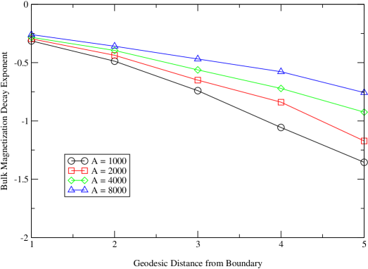
Figure 19: Exponents of bulk magnetization decaying with distance from the boundary at the tricritical point.

7 Conclusion

We have mapped the phase diagram corresponding to a model of Ising spins on a fluctuating geometry with disk topology. At zero boundary magnetic field $H$ we find three phases separated by critical lines on which either the magnetic or boundary length susceptibilities are divergent with disk area. Only one of these phase boundary lines corresponds to continuous transitions — the line separating ferromagnetic and paramagnetic phases on geometries with small mean boundary length. The measured exponent for this transition compares well with predictions from Liouville theory. The third phase consists of elongated geometries whose boundary length scales linearly with disk area. The continuum limit is thought to reside at the junction of the these two critical lines — a tricritical point at which the spins display long range correlations and the mean boundary size scales as the square root of the area $\left<l\right>\sim\sqrt{A}$.

We have tested the results of our simulations in two ways; by comparison to hand counted amplitudes for small disks including the Ising sector and by a direct computation of the critical exponents governing the pure gravity disk partition function. The latter constitutes the first numerical check on the values of these exponents and was accomplished by a measurement of the baby universe distribution (defined now for disk topology) and the density of 3-fold coordinated vertices. In both cases good agreement with predictions was obtained.

We have also computed the dependence of the bulk and boundary magnetizations and susceptibilities on the boundary field $H$ at the tricritical point. We find the boundary magnetization is independent of boundary length or bulk disk area and varies smoothly with $H$. The corresponding susceptibility approaches a constant as $H\to 0$ for large area. Both of these conclusions are consistent with the predictions of a matrix model calculation of a similar model by Carroll, Ortiz and Taylor [4, 5, 6] and at least in the case of the susceptibility differ qualitatively from the situation in flat space.

In the thermodynamic limit and at the tricritical point, a typical bulk spin will be situated infinitely far from the boundary and thus we might expect the critical behavior of the bulk magnetization and susceptibility to be same as on a sphere independent of the boundary field. Our numerical data for the bulk susceptibility is indeed consistent with this — for a wide range of fields $H$ we see a power law dependence on the area with exponent in the range $0.6-0.7$ (the continuum/matrix model prediction is $\frac{2}{3}$). The analysis of the magnetization data is more complicated — a naive power law fit of the area dependence at fixed $H$ yields an exponent of approximately $0.1$ which appears quite different from the predicted value of $\frac{1}{6}$. To explain this we must assume that the influence of the boundary spins induces large finite size corrections in this exponent.

One conjecture made in the paper of Carroll et al. appears to be false — when we measure the bulk magnetization we find that it increases with applied field — contrary to the rather surprising result of the matrix model calculation where a decrease of bulk magnetization with increasing boundary field was found. In that case it was conjectured that the physical interpretation of that result was due to the appearance of a ‘neck’ in the disk geometry which allowed the average bulk spin to be pushed further out from the boundary with increasing field. In our case we have verified that the opposite is true — the average bulk spin is drawn closer to the boundary with increasing field. The explanation for this discrepancy appears to stem from a lack of universality in the calculations — our lattice ensemble differs from the one used in the analytical calculation and renders detailed comparison between the two problematical. Specifically, the function $\alpha(H)$ which induces this result is clearly not universal in character. Further tests of universality obtained by placing the Ising spins on triangles are currently underway.

On a more positive note we have checked another conjecture made in the matrix model paper which speculates that the decay of the boundary magnetization into its value in the bulk is governed by a universal power of the geodesic distance to the boundary where the power law exponent is related to the dressed magnetic exponent of 2-d quantum gravity. We have measured both the number of vertices and the magnetization as a function of geodesic distance from the boundary and found that they exhibit finite size scaling forms for geometries close to the tricritical point. Just as on the sphere it appears that these functions reveal the existence of a single length scale $\xi\sim A^{\frac{1}{d_{H}}}$ governing the behavior of the average number of points and magnetization as we move from the boundary into the interior of the disk. Indeed, the fractal dimension $d_{H}$ appears to be close to its value on the sphere for critical Ising spins coupled to gravity and lends support to the idea that the dressing of Ising spin operators will just follow the KPZ predictions. However, we find the extracted value of the bulk magnetic operator differs from its exact value which we attribute to large residual finite size corrections.

It would also be interesting to see which of these qualitative features carried over to the case of the 3-state Potts model coupled to 2-d gravity on the disk.

8 Acknowledgements

This research was supported by the Department of Energy, USA, under contract number DE-FG02-85ER40237 and by research funds from Syracuse University.

References

- [1] V. A. Kazakov, “Exactly solvable models of 2d-quantum gravity on the lattice,” in Les Houches, Session XLIX, Fields, Strings and Critical Phenomena, E. Brezin and J. Zinn-Justin, eds., p. 369. 1988.
- [2] F. David, “Simplicial quantum gravity and random lattices,” in Les Houches, Session LVII, Gravitation and Quantizations, B. Julia and J. Zinn-Justin, eds., p. 679. 1995.
- [3] J. Ambjørn, J. Jurkiewicz, and Y. Watabiki, “Dynamical triangulations, a gateway to quantum gravity?,” J. Math. Phys. 36 (1995) 6299, hep-th/9503108.
- [4] S. M. Carroll, M. E. Ortiz, and W. Taylor IV, “Boundary fields and renormalization group flow in the two-matrix model,” Phys. Rev. D58 (1998) 046006, hep-th/9711008.
- [5] S. M. Carroll, M. E. Ortiz, and W. Taylor IV, “The ising model with a boundary magnetic field on a random surface,” Phys. Rev. Lett. 77 (1996) 3947, hep-th/9605169.
- [6] S. M. Carroll, M. E. Ortiz, and W. Taylor IV, “A geometric approach to free variable loop equations in discretized theories of 2d gravity,” Nucl. Phys. B468 (1996) 383, hep-th/9510199.
- [7] E. Ising Z. Physik 31 (1925) 253.
- [8] S. Catterall, “Simulations of dynamically triangulated gravity - an algorithm for arbitrary dimensions,” Comp. Phys. Comm. 87 (1995) 409.
- [9] N. Metropolis, A. W. Rosenbluth, M. N. Rosenbluth, A. H. Teller, and E. Teller, “Equation of state calculations by fast computing machines,” J. Chem. Phys. 21 (1953) 1087.
- [10] U. Wolff, “Collective monte carlo updating for spin systems,” Phys. Rev. Lett. 62 (1989) 361.
- [11] W. T. Tutte, “A census of planar triangulations,” Can. J. Math. 14 (1962) 21.
- [12] G. Moore, N. Seiberg, and M. Staudacher, “From loops to states in two-dimensional quantum gravity,” Nucl. Phys. B362 (1991) 665.
- [13] M. Bowick, M. Falcioni, G. Harris, and E. Marinari, “Two ising models coupled to 2-dimensional gravity,” Nucl. Phys. B419 (1994) 665, hep-th/9310136.
- [14] B. M. McCoy and T. T. Wu, “The two dimensional ising model,” Phys. Rev. 77 (1967) 436.
- [15] J. Ambjørn and K. N. Anagnostopoulos, “Quantum geometry of 2d gravity coupled to unitary matter,” Nucl. Phys. B497 (1997) 445, hep-lat/9701006.
- [16] V. G. Knizhnik, A. M. Polyakov, and A. B. Zamolodchikov, “Fractal structure of 2d-quantum gravity,” Mod. Phys. Lett. A3 (1988) 819.