DESY 01-036
HU-EP-01/10
A lattice evaluation of four-quark operators in the nucleon

Abstract

Nucleon matrix elements of various four-quark operators are evaluated in quenched lattice QCD using Wilson fermions. Some of these operators give rise to twist-four contributions to nucleon structure functions. Furthermore, they bear valuable information about the diquark structure of the nucleon. Mixing with lower-dimensional operators is avoided by considering appropriate representations of the flavour group. We find that for a certain flavour combination of baryon structure functions, twist-four contributions are very small. This suggests that twist-four effects for the nucleon might be much smaller than $m_{p}^{2}/Q^{2}$.

, , , , , , and

1 Introduction

The knowledge of higher quark and gluon correlators in hadrons is of fundamental interest in order to understand the structure of baryons and mesons on the basis of QCD. Matrix elements of four-quark operators contain information on the quark and diquark structure of the nucleon. Within the operator product expansion (OPE), four-quark operators give rise to higher-twist contributions (cat’s-ear diagram). While this has been known for many years [1, 2, 3, 4, 5, 6], the size of these contributions is still uncertain. Because the structure function $F_{2}(x,Q^{2})$ of the proton is one of the best measured hadronic quantities, the natural idea would be to extract the higher-twist contribution from the $Q^{2}$ dependence of $F_{2}$. This has, however, proven to be a difficult task (for a recent attempt see Ref. [7]).

A computation of higher-twist effects from first principles is possible by means of Monte Carlo simulations of lattice QCD, and first estimates using this method in the case of the pion became available recently [8]. In this paper we shall extend our previous work to the case of the nucleon.

By means of the OPE $F_{2}(x,Q^{2})$ can be expressed through forward nucleon matrix elements of local operators. In the deep inelastic limit $Q^{2}\to\infty$ it is dominated by the leading twist-two contributions. These have been the subject of intensive studies in the past. The next-to-leading contributions have twist four and are suppressed by one power of $1/Q^{2}$. More precisely, the OPE relates (Nachtmann) moments [9] $\int_{0}^{1}\mathrm{d}x\,x^{n-2}F_{2}(x,Q^{2})\big{|}_{\mathrm{Nachtmann}}$, which take into account the effects of the finite proton mass $m_{p}$, to the product of Wilson coefficients and hadronic matrix elements. Schematically one finds for $n=2,4,6,\ldots$

$$\int_{0}^{1} \mathrm{d}x\,x^{n-2}F_{2}(x,Q^{2})\big{|}_{\mathrm{Nachtmann}}$$ (1)

$$\equiv \int_{0}^{1}\frac{\mathrm{d}x}{x^{3}}\xi^{n+1}F_{2}(x,Q^{2})\big{[}n^{2}+2n+3+3(n+1)(1+4m_{p}^{2}x^{2}/Q^{2})^{1/2}$$

$${}+n(n+2)4m_{p}^{2}x^{2}/Q^{2}\big{]}/(n+2)(n+3)$$

$$= c^{(2)}_{n}(Q^{2}/\mu^{2},g(\mu))A^{(2)}_{n}(\mu)+\frac{c^{(4)}_{n}(Q^{2}/\mu^{2},g(\mu))}{Q^{2}}A^{(4)}_{n}(\mu)+O\left(\frac{1}{Q^{4}}\right)$$

with $\xi=2x/(1+\sqrt{1+4m_{p}^{2}x^{2}/Q^{2}})$.

The reduced matrix elements $A^{(t)}_{n}$ of twist $t$ and spin $n$ depend on the renormalisation scale $\mu$. The mass dimension of $A^{(t)}_{n}$ is $t-2$. The dimensionless Wilson coefficients $c^{(t)}_{n}$ can be calculated in perturbation theory. In the flavour-nonsinglet channel, the twist-two operators are two-quark operators,

$$\bar{\psi}\gamma_{\mu_{1}}\overset{\leftrightarrow}{D}_{\mu_{2}}\cdots\overset{\leftrightarrow}{D}_{\mu_{n}}\psi\,,$$ (2)

symmetrised in all indices and with trace terms subtracted.

The four-quark operators we are interested in have twist four and higher. In particular, the twist-four, spin-two matrix element $A^{(4)}_{2}$ is given by (indices in $\{\dots\}$ are symmetrised)

$$\frac{1}{2}\sum_{S}\langle P,S|A^{c}_{\{\mu\nu\}}-\mbox{trace}|P,S\rangle\equiv\langle P|A^{c}_{\{\mu\nu\}}-\mbox{trace}|P\rangle=2A^{(4)}_{2}(P_{\mu}P_{\nu}-\mbox{trace})$$ (3)

with the four-quark operator

$$A^{c}_{\mu\nu}=(\bar{\psi}G\gamma_{\mu}\gamma_{5}t^{a}\psi)(\bar{\psi}G\gamma_{\nu}\gamma_{5}t^{a}\psi)$$ (4)

(using the nomenclature introduced in Ref. [8]). The quark field $\psi$ carries flavour, colour, and Dirac indices, the matrices $t^{a}$ are the usual generators of colour SU(3)_c, and for two flavours the flavour matrix $G$ reads

$$G=\mbox{diag}(e_{u},e_{d})=\mbox{diag}(2/3,-1/3)$$ (5)

in terms of the quark charges $e_{q}$. The proton states with momentum $P$ and spin vector $S$ are normalised such that

$$\langle P,S|P^{\prime},S^{\prime}\rangle=(2\pi)^{3}2E_{P}\delta({\mathbf{P}}-{\mathbf{P}^{\prime}})\delta_{SS^{\prime}}$$ (6)

The Wilson coefficient reads [4, 5] $c_{2}^{(4)}=g^{2}\left(1+O(g^{2})\right)$.

These expressions are to be compared with their twist-two counterparts:

$$\langle P|\mathcal{O}_{\{\mu\nu\}}-\mbox{trace}|P\rangle=2A^{(2)}_{2}(P_{\mu}P_{\nu}-\mbox{trace})$$ (7)

with the operator

$$\mathcal{O}_{\mu\nu}=\frac{{\mathrm{i}}}{2}\bar{\psi}G^{2}\gamma_{\mu}\overset{\leftrightarrow}{D}_{\nu}\psi$$ (8)

and the Wilson coefficient $c_{2}^{(2)}=1+O(g^{2})$.

The operators (4) and (8) transform identically under Lorentz transformations, but (4) has dimension six, whereas (8) has only dimension four: four-quark operators will in general mix with two-quark operators of lower dimension. This fact complicates the investigation of four-quark operators, because the mixing with lower-dimensional operators cannot be calculated reliably within perturbation theory. A nonperturbative computation in lattice QCD could proceed along the same lines as in the case of the twist-three matrix element $d_{2}$ [10]. For the time being, we do not attempt such a nonperturbative calculation of the renormalisation and mixing coefficients of four-quark operators. Instead we restrict ourselves to cases where mixing with lower-dimensional operators is prohibited by flavour symmetry.

We shall present results obtained in the quenched approximation of lattice QCD with Wilson fermions. A preliminary account of some of these results has already been given in Ref. [11]. Since the lattice formulation of gauge theories requires an analytic continuation from Minkowski space to Euclidean space, we now switch to the Euclidean formulation. In particular, all operators will be written down in Euclidean space, unless otherwise noted.

2 The general framework

In our previous publication [8] we have studied four-quark operators in the pion. In this case we could avoid mixing with lower-dimensional operators by working with operators which carry isospin $I=2$. Obviously, operators with $I=2$ vanish in the proton. Therefore we enlarge the flavour symmetry group from SU(2)_F to SU(3)_F assuming three quarks of the same mass. Correspondingly, we then have

$$G=\mbox{diag}(e_{u},e_{d},e_{s})=\mbox{diag}(2/3,-1/3,-1/3)$$ (9)

and the flavour structure of the operator in the OPE is now

$$\mathcal{O}=(e_{u}\bar{u}u+e_{d}\bar{d}d+e_{s}\bar{s}s)(e_{u}\bar{u}u+e_{d}\bar{d}d+e_{s}\bar{s}s)\,.$$ (10)

While two-quark operators transform under SU(3)_F according to $\overline{\mathbf{3}}\otimes\mathbf{3}=\mathbf{1}\oplus\mathbf{8}$, we have for four-quark operators: $(\overline{\mathbf{3}}\otimes\mathbf{3})\otimes(\overline{\mathbf{3}}\otimes\mathbf{3})=2\cdot\mathbf{1}\oplus 4\cdot\mathbf{8}\oplus\mathbf{10}\oplus\overline{\mathbf{10}}\oplus\mathbf{27}$. Four-quark operators with $I=0,1$, $I_{3}=0$, and hypercharge $Y=0$ belonging to the multiplets $\mathbf{10}$, $\overline{\mathbf{10}}$, $\mathbf{27}$ do not mix with two-quark operators and do not automatically vanish in a proton expectation value. The operators belonging to the $\mathbf{27}$ multiplet are (giving only the flavour structure)

$$\begin{split}\mathcal{O}^{I=1}_{\bf{27}}=&\frac{1}{10}(e_{u}^{2}-e_{d}^{2}-2e_{u}e_{s}+2e_{d}e_{s})[(\bar{u}u)(\bar{u}u)-(\bar{d}d)(\bar{d}d)\\ &-(\bar{u}s)(\bar{s}u)-(\bar{s}u)(\bar{u}s)+(\bar{d}s)(\bar{s}d)+(\bar{s}d)(\bar{d}s)\\ &-(\bar{s}s)(\bar{u}u)-(\bar{u}u)(\bar{s}s)+(\bar{s}s)(\bar{d}d)+(\bar{d}d)(\bar{s}s)]\ ,\end{split}$$ (11)

$$\begin{split}\mathcal{O}^{I=0}_{\bf{27}}=&\frac{1}{60}(e_{u}^{2}+e_{d}^{2}+e_{u}e_{d}-3e_{u}e_{s}-3e_{d}e_{s}+3e_{s}^{2})\\ &[2(\bar{u}u)(\bar{u}u)+2(\bar{d}d)(\bar{d}d)+(\bar{d}d)(\bar{u}u)+(\bar{d}u)(\bar{u}d)\\ &+(\bar{u}d)(\bar{d}u)+(\bar{u}u)(\bar{d}d)-3(\bar{u}s)(\bar{s}u)-3(\bar{s}u)(\bar{u}s)\\ &-3(\bar{d}s)(\bar{s}d)-3(\bar{s}d)(\bar{d}s)-3(\bar{s}s)(\bar{u}u)-3(\bar{u}u)(\bar{s}s)\\ &-3(\bar{s}s)(\bar{d}d)-3(\bar{d}d)(\bar{s}s)+6(\bar{s}s)(\bar{s}s)]\ .\end{split}$$ (12)

Inserting the values of the quark charges one finds

$$e_{u}^{2}-e_{d}^{2}-2e_{u}e_{s}+2e_{d}e_{s}=e_{u}^{2}+e_{d}^{2}+e_{u}e_{d}-3e_{u}e_{s}-3e_{d}e_{s}+3e_{s}^{2}=1\ .$$ (13)

As the operators belong to the same multiplet, the Wigner–Eckart theorem tells us that the proton matrix elements of these two operators are proportional to each other:

$$\langle P|\mathcal{O}^{I=0}_{\mathbf{27}}|P\rangle=\frac{1}{2}\langle P|\mathcal{O}^{I=1}_{\mathbf{27}}|P\rangle\,.$$ (14)

Furthermore, the Wigner–Eckart theorem relates proton matrix elements to neutron matrix elements. Thus our results can easily be rephrased in terms of neutron expectation values. However, unless otherwise stated, we shall only present the proton results.

The operators belonging to the multiplets ${\bf 10}$ and $\overline{\bf{10}}$ read

$$\begin{split}\mathcal{O}_{\mathbf{10}}^{I=1}=&(\bar{d}d)(\bar{u}u)-(\bar{d}u)(\bar{u}d)+(\bar{u}d)(\bar{d}u)-(\bar{u}u)(\bar{d}d)\\ &+(\bar{u}u)(\bar{s}s)+(\bar{d}s)(\bar{s}d)-(\bar{d}d)(\bar{s}s)-(\bar{u}s)(\bar{s}u)\\ &-(\bar{s}d)(\bar{d}s)+(\bar{s}u)(\bar{u}s)+(\bar{s}s)(\bar{d}d)-(\bar{s}s)(\bar{u}u)\ ,\end{split}$$ (15)

$$\begin{split}\mathcal{O}_{\overline{\mathbf{10}}}^{I=1}=&(\bar{d}d)(\bar{u}u)+(\bar{d}u)(\bar{u}d)-(\bar{u}d)(\bar{d}u)-(\bar{u}u)(\bar{d}d)\\ &+(\bar{u}u)(\bar{s}s)-(\bar{d}s)(\bar{s}d)-(\bar{d}d)(\bar{s}s)+(\bar{u}s)(\bar{s}u)\\ &+(\bar{s}d)(\bar{d}s)-(\bar{s}u)(\bar{u}s)+(\bar{s}s)(\bar{d}d)-(\bar{s}s)(\bar{u}u)\ .\end{split}$$ (16)

Being antisymmetric with respect to the interchange of the two quark-antiquark pairs they do not appear in the flavour decomposition of the OPE operator (10).

In the following we present Monte Carlo data from quenched simulations at $\beta=6.0$ with Wilson fermions on a $16^{3}\times 32$ lattice. We have performed simulations at three different values of the hopping parameter $\kappa=0.1515$, $0.1530$ and $0.1550$ and we have collected about 300 configurations. The statistical errors have been determined by the jackknife method.

Figure 1: Plateau for the bare matrix element of $\mathcal{O}_{\mathbf{27}}^{I=1}$ for the operator $V^{c}_{44}-\mbox{trace}$ (see Eq. (LABEL:eq:defop)), divided by $m_{p}^{4}$, with $\kappa=0.1515$.

The proton matrix elements are computed in the standard fashion from ratios of three-point functions, $\langle B(t)\mathcal{O}(\tau)\bar{B}(0)\rangle$, to two-point functions, $\langle B(t)\bar{B}(0)\rangle$, with the interpolating fields $B$ and $\bar{B}$ of Ref. [12]. For $0\ll\tau\ll t$ this ratio should be independent of $t$:

$$R=\frac{\langle B(t)\mathcal{O}(\tau)B(0)\rangle}{\langle B(t)B(0)\rangle}=\frac{1}{(2\kappa)^{2}2m_{p}}\langle P|\mathcal{O}|P\rangle+\cdots$$ (17)

If we vary $t$ keeping $\tau$ fixed we should therefore find a region where $R$ is constant, i.e. shows a plateau. An example of such a plateau is shown in Fig. 1. We have always chosen $\tau=5$ and the spatial components of the proton momentum have been set to zero. The ratio $R$ equals the matrix element in the lattice normalisation of states and fields. In order to obtain the fields in the continuum normalisation we have to multiply each quark field by $\sqrt{2\kappa}$. To normalise the states according to Eq. (6) we must multiply $R$ by an additional factor of $2m_{p}$. We determine the matrix elements by fitting the ratio $R$ to a constant in the region $11\leq t\leq 17$.

For a general four-quark operator the three-point function $\langle B(t)\mathcal{O}(\tau)\bar{B}(0)\rangle$ consists of three types of contributions, which can be represented pictorially by the following diagrams

fd1 (60,40) i1 o1 phantomi1,v plainv,v plain,left=90v,v phantomv,o1 v (0.5w,0.8h)v (0.1w,0.3h)v1 (0.9w,0.3h)v2 decoration.shape=circle,decoration.filled=shaded, decoration.size=0.1hv1 decoration.shape=circle,decoration.filled=shaded, decoration.size=0.1hv2 plain,right=.4v2,v1 plain,left=.4v2,v1 plainv2,v1 fd2 (60,40) i1 o1 phantomi1,v phantomv,o1 (0.5w,0.54h)v (0.1w,0.3h)v1 (0.9w,0.3h)v2 decoration.shape=circle,decoration.filled=shaded, decoration.size=0.1hv1 decoration.shape=circle,decoration.filled=shaded, decoration.size=0.1hv2 plain,left=.4v2,v1 plainv2,v1 plain,right=.2v2,v,v1 v plain,tension=1.4v,v

fd3 (60,40) (0.5w,0.54h)v (0.1w,0.3h)v1 (0.9w,0.3h)v2 decoration.shape=circle,decoration.filled=shaded, decoration.size=0.1hv1 decoration.shape=circle,decoration.filled=shaded, decoration.size=0.1hv2 plain,left=.4v2,v1 plain,left=.4v2,v plain,right=.4v2,v plain,left=.4v,v1 plain,right=.4v,v1 v

It is precisely through contributions of the form of the first two diagrams that the mixing with lower-dimensional operators occurs. Therefore these contributions cancel in the operators which we consider, and we are left with the contributions of the last type only. For proton matrix elements only some terms of the operators contribute, e.g. the $(\bar{d}d)(\bar{d}d)$ terms vanish as those containing $s$ quarks. Therefore the expectation values of the operators (11), (15), (16) reduce to

$$\begin{split}\langle P|\mathcal{O}^{I=1}_{\bf{27}}|P\rangle&=\frac{1}{10}\langle P|(\bar{u}u)(\bar{u}u)|P\rangle\big{|}^{\bf 27}\,,\\ \langle P,S|\mathcal{O}^{I=1}_{\bf{10}}|P,S\rangle&=\langle P,S|(\bar{d}d)(\bar{u}u)-(\bar{d}u)(\bar{u}d)+(\bar{u}d)(\bar{d}u)-(\bar{u}u)(\bar{d}d)|P,S\rangle\big{|}^{\bf 10}\,,\\ \langle P,S|\mathcal{O}^{I=1}_{\overline{\bf{10}}}|P,S\rangle&=\langle P,S|(\bar{d}d)(\bar{u}u)+(\bar{d}u)(\bar{u}d)-(\bar{u}d)(\bar{d}u)-(\bar{u}u)(\bar{d}d)|P,S\rangle\big{|}^{\overline{\bf 10}}\,.\end{split}$$ (18)

At each $\kappa$ value the matrix elements are made dimensionless by dividing them by the corresponding value of $m_{p}^{4}$. As the bare quark mass is given by $am_{q}=1/(2\kappa)-1/(2\kappa_{c})$ we perform the chiral limit by linear extrapolation in $1/\kappa$ to $1/\kappa=1/\kappa_{c}=6.3642$. As an example of our results we show in Fig. 2 the chiral extrapolation of the bare proton matrix element of $V^{c}_{44}-\mbox{trace}$ (${I=1}$ component in the $\mathbf{27}$ representation of SU(3)_F) divided by $m_{p}^{4}$. (For the definition of $V^{c}_{\mu\nu}$ see Eq. (LABEL:eq:defop).)

Figure 2: Chiral extrapolation of the bare proton matrix element of $\mathcal{O}^{I=1}_{\mathbf{27}}$ for the operator $V^{c}_{44}-\mbox{trace}$ (see Eq. (LABEL:eq:defop)), divided by $m_{p}^{4}$.

3 Operators from the $\mathbf{27}$ multiplet

The twist-four contribution in the $F_{2}$ structure function comes from the four-quark operator $A_{\mu\nu}^{c}$, see Eq. (4). In order to access the flavour-${\mathbf{27}}$ component experimentally one has to combine the structure functions of several baryons ($p$, $n$, $\Lambda$, $\Sigma$, $\Xi$) in such a way as to project out the desired flavour combination, e.g.

$$\langle p|\mathcal{O}^{I=1}_{\mathbf{27}}|p\rangle = \langle\Sigma^{+}|\mathcal{O}|\Sigma^{+}\rangle-2\langle\Sigma^{0}|\mathcal{O}|\Sigma^{0}\rangle+\langle\Sigma^{-}|\mathcal{O}|\Sigma^{-}\rangle$$ (19)

$$= -\langle\Sigma^{+}|\mathcal{O}|\Sigma^{+}\rangle-\langle\Sigma^{-}|\mathcal{O}|\Sigma^{-}\rangle$$

$$-6\langle\Lambda|\mathcal{O}|\Lambda\rangle+2\langle\Xi^{0}|\mathcal{O}|\Xi^{0}\rangle+2\langle\Xi^{-}|\mathcal{O}|\Xi^{-}\rangle$$

$$+2\langle p|\mathcal{O}|p\rangle+2\langle n|\mathcal{O}|n\rangle\,.$$

Unfortunately most of these terms will not be measured in the foreseeable future. So a direct comparison with data is out of question. On the other hand, they can be used as a testing ground for models of hadrons, taking the role of experimental data. Note that the ${\mathbf{27}}$ contribution can also be isolated by studying combinations of electromagnetic and weak structure functions [13].

Of course, we need to know the renormalised operators. Although due to our choice of the flavour-${\mathbf{27}}$ component mixing with two-quark operators is absent, different four-quark operators may still mix under renormalisation. Therefore we have computed the matrix elements of the following operators (using the nomenclature introduced in Ref. [8]):

$$\begin{split}V^{c}_{\mu\nu}&=\bar{\psi}G\gamma_{\mu}t^{a}\psi\,\bar{\psi}G\gamma_{\nu}t^{a}\psi,\\[2.15277pt] A^{c}_{\mu\nu}&=\bar{\psi}G\gamma_{\mu}\gamma_{5}t^{a}\psi\,\bar{\psi}G\gamma_{\nu}\gamma_{5}t^{a}\psi,\\[2.15277pt] T^{c}_{\mu\nu}&=\bar{\psi}G\sigma_{\mu\rho}t^{a}\psi\,\bar{\psi}G\sigma_{\nu\rho}t^{a}\psi,\\[2.15277pt] V_{\mu\nu}&=\bar{\psi}G\gamma_{\mu}\psi\,\bar{\psi}G\gamma_{\nu}\psi,\\[2.15277pt] A_{\mu\nu}&=\bar{\psi}G\gamma_{\mu}\gamma_{5}\psi\,\bar{\psi}G\gamma_{\nu}\gamma_{5}\psi,\\[2.15277pt] T_{\mu\nu}&=\bar{\psi}G\sigma_{\mu\rho}\psi\,\bar{\psi}G\sigma_{\nu\rho}\psi.\\ \end{split}$$ (20)

The bare expectation values divided by $m_{p}^{4}$ and extrapolated to the chiral limit are given in Table 1 for the the spin-two components, while the traces are given in Table 2. E.g. the number shown for the operator $A^{c}_{\mu\nu}-\mbox{trace}$ in Table 1 is what we obtain for $\langle P|\frac{1}{10}(\bar{u}\gamma_{4}\gamma_{5}t^{a}u)(\bar{u}\gamma_{4}\gamma_{5}t^{a}u)-\mbox{trace}|P\rangle/m_{p}^{4}$ in the chiral limit. We have checked that these operators fulfil their Fierz identities.

Table 1: Matrix elements of the spin-two operators from the ${\mathbf{27}}$ multiplet, divided by $m_{p}^{4}$ and extrapolated to the chiral limit.

operator
$A^{c}_{\{\mu\nu\}}-\mbox{trace}$	$(-0.9\pm 0.8)\cdot 10^{-4}$
$V^{c}_{\{\mu\nu\}}-\mbox{trace}$	$(-4.5\pm 1.0)\cdot 10^{-4}$
$T^{c}_{\{\mu\nu\}}-\mbox{trace}$	$(4.9\pm 0.8)\cdot 10^{-4}$
$A_{\{\mu\nu\}}-\mbox{trace}$	$(-0.0\pm 1.3)\cdot 10^{-4}$
$V_{\{\mu\nu\}}-\mbox{trace}$	$(8.4\pm 1.4)\cdot 10^{-4}$
$T_{\{\mu\nu\}}-\mbox{trace}$	$(-4.6\pm 1.9)\cdot 10^{-4}$

Table 2: Matrix elements of the spin-zero operators from the ${\mathbf{27}}$ multiplet, divided by $m_{p}^{4}$ and extrapolated to the chiral limit.

Dirac structure	$t_{a}\otimes t_{a}$	$1\otimes 1$
$\gamma_{5}\otimes\gamma_{5}$	$(2.8\pm 0.7)\cdot 10^{-4}$	$(-13.4\pm 2.6)\cdot 10^{-4}$
$1\otimes 1$	$(-7.1\pm 1.2)\cdot 10^{-4}$	$(17.8\pm 2.9)\cdot 10^{-4}$
$\gamma_{\mu}\gamma_{5}\otimes\gamma_{\mu}\gamma_{5}$	$(17.2\pm 2.0)\cdot 10^{-4}$	$(-12.1\pm 3.9)\cdot 10^{-4}$
$\gamma_{\mu}\otimes\gamma_{\mu}$	$(-18.2\pm 2.2)\cdot 10^{-4}$	$(7.4\pm 4.0)\cdot 10^{-4}$
$\sigma_{\mu\nu}\otimes\sigma_{\mu\nu}$	$(-4\pm 7)\cdot 10^{-4}$	$(17.6\pm 9.6)\cdot 10^{-4}$

The renormalisation constants have been calculated in one-loop perturbation theory [8]. The renormalised spin-two piece of the operator $A^{c}_{\mu\nu}$ reads

$$\begin{split}\big{[}A^{c}_{\mu\nu}(\mu)\big{]}^{\mathrm{ren}}=A^{c}_{\mu\nu}-\frac{g_{0}^{2}}{16\pi^{2}}\big{[}&\left(3\ln(a\mu)+46.072285\right)A^{c}_{\mu\nu}\\ &+\left(-\frac{8}{9}\ln(a\mu)+0.083982\right)V_{\mu\nu}\\ &+\left(-\frac{5}{3}\ln(a\mu)+0.157467\right)V^{c}_{\mu\nu}\\ &-1.071448\,\,T_{\mu\nu}-2.008965\,\,T^{c}_{\mu\nu}\big{]}\,,\end{split}$$ (21)

where $g_{0}$ is the bare coupling constant ($\beta\equiv 6/g_{0}^{2}$).The renormalisation scale $\mu$ will be identified with the inverse lattice spacing $1/a$. In our simulations this has a value of $1/a\approx 2.12{\,\rm GeV}$ (using $r_{0}$ to set the scale). In terms of the renormalised operator the reduced matrix element $A_{2}^{(4)}$ is then given by

$$\frac{1}{m_{p}^{2}}A^{(4)}_{2}\big{|}^{\rm{\bf 27},I=1}=\frac{2}{3}\frac{\langle P|\frac{1}{10}(\bar{u}\gamma_{4}\gamma_{5}t^{a}u)(\bar{u}\gamma_{4}\gamma_{5}t^{a}u)-\mbox{trace}|P\rangle}{m_{p}^{4}}\,,$$ (22)

and we obtain for the lowest moment of $F_{2}$ in our special flavour channel

$$\int_{0}^{1}\mathrm{d}x\,F_{2}(x,Q^{2})\big{|}_{\mathrm{Nachtmann}}^{\mathbf{27},I=1}=-0.0005(5)\frac{m_{p}^{2}\alpha_{s}(Q^{2})}{Q^{2}}+O(\alpha_{s}^{2})\,.$$ (23)

The analogous result for the neutron differs from the above only by the sign.

In the proton the corresponding twist-two contribution is about $0.14$ at $Q^{2}=5{\,\rm GeV}^{2}$. As in the pion, the twist-four correction is tiny. Our result may be compared with bag model estimates. In this model the scale for the prefactor in Eq. (23) is set by $B/m_{p}^{4}\approx 0.0006$, where $B\approx(145\mbox{MeV})^{4}$ is the bag constant. The factor $B/m_{p}^{4}$ is however multiplied by a relatively large (and negative) number [3].

It is rather difficult to determine the first moment of the higher-twist contribution to $F_{2}(x)$ experimentally. Phenomenological fits to the available data give a positive value of about $0.005(4){\,\rm GeV}^{2}/Q^{2}$ [7, 14]. Our matrix element, which is due to its flavour structure only one contribution to the full moment, is considerably smaller than this phenomenological number.

4 Operators from the $\mathbf{10}$ and $\mathbf{\overline{10}}$ multiplets

Having found rather small matrix elements for our four-quark operators from the $\mathbf{27}$ one may ask if operators from the $\mathbf{10}$ or ${\overline{\mathbf{10}}}$ of $\mathrm{SU}(3)_{\mathrm{F}}$ (although not contributing to $F_{2}$ in the OPE) would have larger matrix elements. With the two possible colour structures that can form colour singlet operators, these operators are linear combinations of terms of the form $(\bar{\psi}G\,\Gamma t^{a}\psi)(\,\bar{\psi}G^{\prime}\,\Gamma^{\prime}t^{a}\psi)$ and $(\bar{\psi}G\,\Gamma\psi)(\,\bar{\psi}G^{\prime}\,\Gamma^{\prime}\psi)$, respectively, where $\Gamma$ and $\Gamma^{\prime}$ are Dirac matrices. We have chosen the flavour matrices $G$, $G^{\prime}$ such that we get the following flavour structures:

$$(\bar{d}d)(\bar{u}u)-(\bar{u}u)(\bar{d}d)$$ (24)

and

$$(\bar{d}u)(\bar{u}d)-(\bar{u}d)(\bar{d}u)\ .$$ (25)

These can be combined to yield the $\mathbf{10}$ and $\overline{\mathbf{10}}$ structures in Eq. (18).

Discrete symmetries impose restrictions on the matrix elements of these operators. We have

$$\langle P,S|\mathcal{O}|P,S\rangle^{*}=\langle P,-S|{\cal{TP}}\mathcal{O}{\cal{P}}^{-1}{\cal T}^{-1}|P,-S\rangle=\langle P,S|\mathcal{O}^{\dagger}|P,S\rangle$$ (26)

where ${\cal P}$ is the parity and ${\cal T}$ is the time inversion operator. For the Dirac matrices used in our computations we define sign factors $s_{1}$, $s_{1}^{\prime}$, $s_{2}$ and $s_{2}^{\prime}$ by

$$\begin{array}[]{ccc}\gamma_{4}\Gamma^{\dagger}\gamma_{4}=s_{1}\Gamma&,&\gamma_{4}{\Gamma^{\prime}}^{\dagger}\gamma_{4}=s_{1}^{\prime}\Gamma^{\prime}\ ,\\ \gamma_{4}\gamma_{5}C\Gamma^{*}C^{-1}\gamma_{5}\gamma_{4}=s_{2}\Gamma&,&\gamma_{4}\gamma_{5}C{\Gamma^{\prime}}^{*}C^{-1}\gamma_{5}\gamma_{4}=s^{\prime}_{2}\Gamma^{\prime}\,.\end{array}$$ (27)

Here $C$ is the charge conjugation matrix with $C\gamma_{\mu}^{\rm T}C^{-1}=-\gamma_{\mu}$. One more sign $\epsilon_{\mathcal{O}}$ is determined by

$$\langle P,-S|\mathcal{O}|P,-S\rangle=\epsilon_{\mathcal{O}}\langle P,S|\mathcal{O}|P,S\rangle\ .$$ (28)

From Eq. (26) we now get for the flavour structure (24)

$$\langle P,S|\mathcal{O}|P,S\rangle^{*}=\epsilon_{\mathcal{O}}s_{2}s_{2}^{\prime}\langle P,S|\mathcal{O}|P,S\rangle=s_{1}s_{1}^{\prime}\langle P,S|\mathcal{O}|P,S\rangle$$ (29)

and for the flavour structure (25)

$$\langle P,S|\mathcal{O}|P,S\rangle^{*}=\epsilon_{\mathcal{O}}s_{2}s_{2}^{\prime}\langle P,S|\mathcal{O}|P,S\rangle=-s_{1}s_{1}^{\prime}\langle P,S|\mathcal{O}|P,S\rangle\ .$$ (30)

Thus the matrix element $\langle P,S|\mathcal{O}|P,S\rangle$ is real if $\epsilon_{\mathcal{O}}s_{2}s_{2}^{\prime}=1$ and purely imaginary if $\epsilon_{\mathcal{O}}s_{2}s_{2}^{\prime}=-1$; the matrix element vanishes if $\epsilon_{\mathcal{O}}s_{2}s_{2}^{\prime}=-s_{1}s_{1}^{\prime}$ for the flavour structure (24) or $\epsilon_{\mathcal{O}}s_{2}s_{2}^{\prime}=s_{1}s_{1}^{\prime}$ for the flavour structure (25). We have checked that these restrictions are satisfied by our results within statistical errors. We restrict ourselves in the following to the matrix elements which are not forced to be zero by the above relations. Note that for a given Dirac structure at most one of the flavour structures (24) and (25) yields a non-vanishing result.

The definite Lorentz transformation properties of our operators could be used to define reduced matrix elements, e.g. in Minkowski space one gets

$$\langle P,S|(\bar{d}\gamma_{\mu}\gamma_{5}d)(\bar{u}\gamma_{\nu}\gamma_{5}u)-(\bar{u}\gamma_{\mu}\gamma_{5}u)(\bar{d}\gamma_{\nu}\gamma_{5}d)|P,S\rangle=A\epsilon_{\mu\nu\alpha\beta}(P^{\alpha}S^{\beta}-S^{\alpha}P^{\beta})\,.$$ (31)

Thus in this case the matrix element with $\mu=1$, $\nu=2$ and $S^{\alpha}=\delta_{\alpha 3}$ is equal to the one with $\mu=2$, $\nu=3$ and $S^{\alpha}=\delta_{\alpha 1}$. This holds only on average, so in order to increase the statistics we averaged over these matrix elements to reduce the statistical error. The bare expectation values divided by $m_{p}^{4}$ are given together with their statistical errors in Tables 3 and 4.

Table 3: Expectation values of operators with the flavour structures (24) and (25) in an unpolarised proton, divided by $m_{p}^{4}$ and extrapolated to the chiral limit.

Dirac structure	flavour	$t_{a}\otimes t_{a}$	$1\otimes 1$
$1\otimes\gamma_{4}$	(24)	$(0.4\pm 0.6)\cdot 10^{-3}$	$(3.0\pm 1.6)\cdot 10^{-3}$
$\epsilon_{4\alpha\beta\delta}\gamma_{\alpha}\gamma_{5}\otimes\sigma_{\beta\delta}$	(24)	$(-5.6\pm 2.8)\cdot 10^{-3}{\mathrm{i}}$	$(5.9\pm 3.6)\cdot 10^{-3}{\mathrm{i}}$
$\gamma_{5}\otimes\gamma_{4}\gamma_{5}$	(25)	$(0.6\pm 0.5)\cdot 10^{-3}$	$(-3.3\pm 1.8)\cdot 10^{-3}$
$\gamma_{\alpha}\otimes\sigma_{4\alpha}$	(25)	$(-3.1\pm 1.2)\cdot 10^{-3}{\mathrm{i}}$	$(0.1\pm 1.9)\cdot 10^{-3}{\mathrm{i}}$

Table 4: Expectation values of operators with the flavour structures (24) and (25) in a polarised proton (${\mathbf{S}}={\mathbf{e}}_{3}$), divided by $m_{p}^{4}$ and extrapolated to the chiral limit.

Dirac structure	flavour	$t_{a}\otimes t_{a}$	$1\otimes 1$
$1\otimes\gamma_{3}\gamma_{5}$	(24)	$(-3.3\pm 0.6)\cdot 10^{-3}{\mathrm{i}}$	$(15.9\pm 1.6)\cdot 10^{-3}{\mathrm{i}}$
$1\otimes\sigma_{21}$	(24)	$(-4.1\pm 0.6)\cdot 10^{-3}$	$(10.7\pm 1.8)\cdot 10^{-3}$
$\gamma_{5}\otimes\sigma_{43}$	(24)	$(2.2\pm 0.5)\cdot 10^{-3}$	$(-4.4\pm 1.3)\cdot 10^{-3}$
$\gamma_{4}\otimes\gamma_{3}\gamma_{5}-\gamma_{3}\otimes\gamma_{4}\gamma_{5}$	(24)	$(-9.1\pm 0.9)\cdot 10^{-3}{\mathrm{i}}$	$(13.0\pm 2.1)\cdot 10^{-3}{\mathrm{i}}$
$\epsilon_{3\alpha\lambda\rho}\gamma_{\alpha}\otimes\sigma_{\lambda\rho}$	(24)	$(42\pm 4)\cdot 10^{-3}$	$(-51\pm 5)\cdot 10^{-3}$
$\gamma_{5}\otimes\gamma_{3}$	(25)	$(4.9\pm 0.5)\cdot 10^{-3}{\mathrm{i}}$	$(-15.6\pm 1.4)\cdot 10^{-3}{\mathrm{i}}$
$\gamma_{2}\otimes\gamma_{1}$	(25)	$(2.4\pm 0.5)\cdot 10^{-3}{\mathrm{i}}$	$(-5.6\pm 0.9)\cdot 10^{-3}{\mathrm{i}}$
$\gamma_{2}\gamma_{5}\otimes\gamma_{1}\gamma_{5}$	(25)	$(6.1\pm 0.8)\cdot 10^{-3}{\mathrm{i}}$	$(-7.6\pm 1.1)\cdot 10^{-3}{\mathrm{i}}$
$\gamma_{\alpha}\gamma_{5}\otimes\sigma_{3\alpha}$	(25)	$(21.5\pm 1.8)\cdot 10^{-3}$	$(-19.2\pm 2.6)\cdot 10^{-3}$
$\sigma_{2\alpha}\otimes\sigma_{1\alpha}$	(25)	$(-8.9\pm 1.5)\cdot 10^{-3}{\mathrm{i}}$	$(8.1\pm 1.8)\cdot 10^{-3}{\mathrm{i}}$

The order of magnitude of the results does not differ greatly from those found for the operators in the $\mathbf{27}$. The renormalisation constants for the $\mathbf{10}$ and $\overline{\mathbf{10}}$ operators are not known, but we do not expect that the renormalised operators have much larger matrix elements than the bare ones.

5 Diquarks

The four-quark operators can be rewritten to look like a diquark density. We have computed matrix elements of operators of the following form:

$$\frac{1}{10}(\bar{u}_{a}\Gamma\gamma_{5}C\bar{u}_{b}^{\rm T})(u_{a^{\prime}}^{\rm T}C^{-1}\gamma_{5}\Gamma^{\prime}u_{b^{\prime}})(\delta_{ab^{\prime}}\delta_{ba^{\prime}}-\delta_{aa^{\prime}}\delta_{bb^{\prime}})\,,$$ (32)

$$\frac{1}{10}(\bar{u}_{a}\Gamma\gamma_{5}C\bar{u}_{b}^{\rm T})(u_{a^{\prime}}^{\rm T}C^{-1}\gamma_{5}\Gamma^{\prime}u_{b^{\prime}})(\delta_{ab^{\prime}}\delta_{ba^{\prime}}+\delta_{aa^{\prime}}\delta_{bb^{\prime}})\,,$$ (33)

where $a$, $b$, $a^{\prime}$ and $b^{\prime}$ are the colour indices. These are the two possibilities to form a colour singlet. In Eq. (32) the diquark is in a $\overline{\mathbf{3}}$ of colour and thus anti-symmetric in colour. In Eq. (33) it is in a ${\mathbf{6}}$ and symmetric in colour. Because of the Pauli principle it has to be symmetric (anti-symmetric) in the other indices. The flavour structure being symmetric, the Dirac structure has therefore to be symmetric (anti-symmetric). Thus a given Dirac structure will appear only for one of the two possible colour structures. The expectation values of operators of the form (32) and (33) can be computed from those of the four-quark operators studied in Section 3. But in order to get the correct errors we have redone the analysis. The results (again divided by $m_{p}^{4}$) are presented in Tables 5 and 6 for the spin-zero and the spin-two contributions, respectively.

Table 5: Matrix elements of the spin-zero operators from the $\mathbf{27}$ multiplet in the diquark picture, divided by $m_{p}^{4}$ and extrapolated to the chiral limit.

operator	colour
$\frac{1}{10}(\bar{u}\gamma_{\mu}\gamma_{5}\gamma_{5}C\bar{u}^{\rm T})(u^{\rm T}C^{-1}\gamma_{5}\gamma_{\mu}\gamma_{5}u)$	$\overline{\mathbf{3}}$	$(-83\pm 8)\cdot 10^{-4}$
$\frac{1}{10}(\bar{u}\sigma_{\mu\nu}\gamma_{5}C\bar{u}^{\rm T})(u^{\rm T}C^{-1}\gamma_{5}\sigma_{\mu\nu}u)$	$\overline{\mathbf{3}}$	$(42\pm 22)\cdot 10^{-4}$
$\frac{1}{10}(\bar{u}\gamma_{\mu}\gamma_{5}C\bar{u}^{\rm T})(u^{\rm T}C^{-1}\gamma_{5}\gamma_{\mu}u)$	${\mathbf{6}}$	$(45\pm 9)\cdot 10^{-4}$
$\frac{1}{10}(\bar{u}\gamma_{5}\gamma_{5}C\bar{u}^{\rm T})(u^{\rm T}C^{-1}\gamma_{5}\gamma_{5}u)$	${\mathbf{6}}$	$(-0.8\pm 2.6)\cdot 10^{-4}$
$\frac{1}{10}(\bar{u}\gamma_{5}C\bar{u}^{\rm T})(u^{\rm T}C^{-1}\gamma_{5}u)$	${\mathbf{6}}$	$(-4.9\pm 6.7)\cdot 10^{-4}$

Table 6: Matrix elements of the spin-two operators from the $\mathbf{27}$ multiplet in the diquark picture, divided by $m_{p}^{4}$ and extrapolated to the chiral limit.

operator	colour
$\frac{1}{10}(\bar{u}\gamma_{4}\gamma_{5}\gamma_{5}C\bar{u}^{\rm T})(u^{\rm T}C^{-1}\gamma_{5}\gamma_{4}\gamma_{5}u)-\mbox{trace}$	$\overline{\mathbf{3}}$	$(12.9\pm 2.2)\cdot 10^{-4}$
$\frac{1}{10}(\bar{u}\sigma_{4\alpha}\gamma_{5}C\bar{u}^{\rm T})(u^{\rm T}C^{-1}\gamma_{5}\sigma_{4\alpha}u)-\mbox{trace}$	$\overline{\mathbf{3}}$	$(-16.8\pm 4.3)\cdot 10^{-4}$
$\frac{1}{10}(\bar{u}\gamma_{4}\gamma_{5}C\bar{u}^{\rm T})(\bar{u}^{\rm T}C^{-1}\gamma_{5}\gamma_{4}u)-\mbox{trace}$	${\mathbf{6}}$	$(3.9\pm 2.9)\cdot 10^{-4}$

Strictly speaking, we are again studying operators from the ${\mathbf{27}}$ representation of ${\mathrm{SU}}(3)_{\mathrm{F}}$, whose $\bar{u}\bar{u}uu$ component is given by Eqs. (32) and (33), respectively. At least within the quenched approximation it seems however reasonable to consider (32) and (33) as representing valence diquark densities. In the same spirit, one could also investigate $ud$ diquarks. But due to flavour symmetry (see Eq. (14)) the corresponding matrix elements are proportional to those of the $uu$ diquarks (32) and (33). Writing down only the flavour structure one finds for the expectation values in the proton

$$\langle P|(\bar{u}\bar{d}^{\,{\rm T}})(d^{\rm T}u)|P\rangle=\frac{1}{4}\langle P|(\bar{u}\bar{u}^{\rm T})(u^{\rm T}u)|P\rangle.$$ (34)

In order to interpret our results we have combined operators from Tables 5 and 6 such that they correspond to diquarks of spin zero and spin one. Specifically, for an operator $\mathcal{O}_{\mu\nu}$ with two space-time indices we take the expectation value of $\mathcal{O}_{44}$ to represent a spin-zero diquark and the expectation value of $\sum_{i=1}^{3}\mathcal{O}_{ii}$ to correspond to a spin-one diquark. The results (once again completely reanalysed) are given in Table 7.

Table 7: Expectation values of operators from the $\mathbf{27}$ multiplet which correspond to diquarks of spin zero and spin one, divided by $m_{p}^{4}$ and extrapolated to the chiral limit. For the operator $\mathcal{O}_{\mu\nu}$ the spin-zero contribution is $\mathcal{O}_{44}$, the spin-one contribution is $\sum_{i=1}^{3}\mathcal{O}_{ii}$.

operator	colour	spin 0	spin 1
$\frac{1}{10}(\bar{u}\gamma_{\mu}\gamma_{5}\gamma_{5}C\bar{u}^{\rm T})(u^{\rm T}C^{-1}\gamma_{5}\gamma_{\nu}\gamma_{5}u)$	$\overline{\mathbf{3}}$	$(-6.8\pm 2.4)\cdot 10^{-4}$	$(-76\pm 7)\cdot 10^{-4}$
$\frac{1}{10}(\bar{u}\sigma_{\mu\alpha}\gamma_{5}C\bar{u}^{\rm T})(u^{\rm T}C^{-1}\gamma_{5}\sigma_{\nu\alpha}u)$	$\overline{\mathbf{3}}$	$(-5.7\pm 6.1)\cdot 10^{-4}$	$(48\pm 18)\cdot 10^{-4}$
$\frac{1}{10}(\bar{u}\gamma_{\mu}\gamma_{5}C\bar{u}^{\rm T})(\bar{u}^{\rm T}C^{-1}\gamma_{5}\gamma_{\nu}u)$	${\mathbf{6}}$	$(15.0\pm 3.6)\cdot 10^{-4}$	$(30\pm 7)\cdot 10^{-4}$

For the operators in the ${\bf\overline{3}}$ of colour the absolute values for the spin-one diquarks are considerably larger than for the spin-zero diquarks. For the single operator in the ${\bf 6}$ of colour the difference is less pronounced. This pattern can tentatively be understood in a non-relativistic quark picture. When the diquark is in the ${\bf\overline{3}}$ of SU(3)_c it is anti-symmetric in the colour indices, and therefore the symmetric (in the spin indices) spin-one state is favoured over the anti-symmetric spin-one state. On the other hand, when the diquark is in the (symmetric) ${\bf 6}$ of colour one might at first sight expect the anti-symmetric spin-zero state to dominate over the symmetric spin-one state. Although the spin-zero contribution is indeed less suppressed than in the ${\bf\overline{3}}$ case it is not really dominating. This is probably related to the fact that a diquark in the ${\bf 6}$ of SU(3)_c must be accompanied by (at least) one gluon if it is to form a colour singlet with the remaining quark. The coupling to the gluon, mixing “large” and “small” components of the quark spinors, would invalidate the above arguments which worked reasonably well for diquarks in the ${\bf\overline{3}}$ of colour.

Of course, the operators from the ${\mathbf{10}}$ and ${\overline{\mathbf{10}}}$ multiplets can also rewritten in diquark form. They then appear as linear combinations of operators in which the diquark is either in a ${\bf\overline{3}}$ of SU(3)_c or in a ${\mathbf{6}}$. The fact that the matrix elements in Table 4 for the colour structures $t_{a}\otimes t_{a}$ and $1\otimes 1$ have opposite signs translates into a suppression of the ${\mathbf{6}}$ diquarks relative to the ${\bf\overline{3}}$ diquarks. This is in accord with our observations made above in the case of the operators from the ${\mathbf{27}}$ multiplet.

6 Summary

In this paper we have computed the expectation values of a variety of four-quark operators in the proton by means of quenched Monte Carlo simulations. Since it is rather difficult to treat the mixing with lower-dimensional operators correctly, we have restricted ourselves to operators whose flavour structure forbids this kind of mixing. The additional requirement that the operators should not automatically vanish in the nucleon led us to consider the flavour group SU(3)_F and to choose operators from the ${\bf 27}$, ${\bf 10}$, and ${\bf\overline{10}}$ representations. One of the operators from the ${\bf 27}$ is responsible for the twist-four contribution to the lowest moment of $F_{2}$ in a somewhat exotic flavour channel. We find a rather small value for this contribution. This observation disfavours large higher-twist effects in general, although we cannot exclude, of course, that our result is due to strong cancellations between different flavour contributions.

Still, and with all due caution, our findings fit into a general trend emerging from various pieces of information on higher-twist contributions to moments of nucleon structure functions: The natural energy scale for the corresponding correlators lies well below the nucleon mass leading to small numerical coefficients when the matrix elements are expressed as multiples of $(m_{p})^{t-2}$.

Thus we arrive for the nucleon at a conclusion which is similar to what we observed in the pion [8]. For a more detailed comparison we plot in Fig. 3 the renormalised pion matrix elements [8] with the flavour structure

$$\begin{split}\langle\pi^{+}|(\bar{u}u)(\bar{u}u)+(\bar{d}d)(\bar{d}d)&-(\bar{u}u)(\bar{d}d)-(\bar{d}d)(\bar{u}u)\\ &-(\bar{u}d)(\bar{d}u)-(\bar{d}u)(\bar{u}d)|\pi^{+}\rangle/m_{\pi}^{2}\end{split}$$ (35)

together with the corresponding renormalised matrix elements for the proton $\langle p|10\cdot\mathcal{O}^{I=1}_{\bf 27}|p\rangle/m_{p}^{2}$ (in lattice units). We display the results for the spin-two components setting $\mu=\nu=4$ (with the trace term subtracted). The normalisation of the operators is chosen such that the flavour structure $(\bar{u}u)(\bar{u}u)$ appears with the factor 1 in both cases. (Alternatively, it may be remarked that SU(3)_F makes the above pion matrix element equal to the expectation value of $10\cdot\mathcal{O}^{I=1}_{\bf 27}$ in the meson-octet analogue of the proton, the $K^{+}$.) It is no great surprise that the numbers do not show many similarities – after all, the pion and the proton are very different particles.

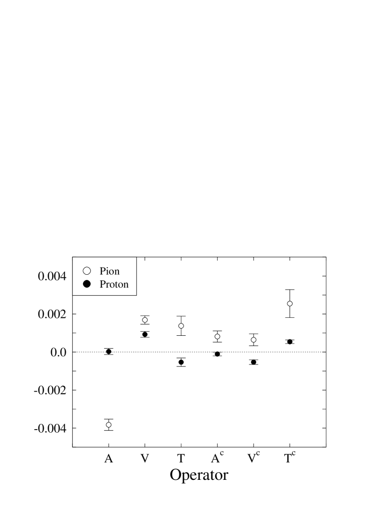
Figure 3: Renormalised four-quark matrix elements in the pion and in the proton (in lattice units).

Four-quark operators in the ${\bf 10}$ and ${\bf\overline{10}}$ representations do not lead to much larger matrix elements than the ${\bf 27}$ operators, although quite a few of those which we studied give clean signals. In the ${\bf 27}$ sector, a rewriting of our operators in terms of diquarks reveals a structure which lends itself to an interpretation with the help of quark model ideas: Diquarks in the $\overline{\bf 3}$ of SU(3)_c have preferably spin one. Diquarks in the ${\bf 6}$ of SU(3)_c, on the other hand, do not fit so well into a nonrelativistic picture.

Higher-twist effects will challenge lattice QCD for a few more years. Our investigations show that four-quark operators can give reasonable signals in present quenched Monte Carlo simulations. But the study of physically more interesting flavour channels and further twist-four operators remains an open problem whose solution requires progress in nonperturbative renormalisation, especially in the treatment of mixing with operators of lower dimension.

References

• [1] S.P. Luttrell, S. Wada and B.R. Webber, Nucl. Phys.  B188 (1981) 219;
S.P. Luttrell and S. Wada, Nucl. Phys.  B197 (1982) 290; ibid. B206 (1982) 497 (E).
• [2] R.K. Ellis, W. Furmański and R. Petronzio, Nucl. Phys.  B207 (1982) 1; ibid. B212 (1983) 29.
• [3] R.L. Jaffe and M. Soldate, Phys. Lett. B105 (1981) 467.
• [4] R. L. Jaffe and M. Soldate, Phys. Rev. D26 (1982) 49.
• [5] E. V. Shuryak and A. I. Vainshtein, Nucl. Phys.  B199 (1982) 451.
• [6] J.L. Miramontes and J. Sánchez Guillén, Z. Phys. C41 (1988) 247.
• [7] S. I. Alekhin, hep-ph/0011002 and private communication.
• [8] S. Capitani, M. Göckeler, R. Horsley, B. Klaus, V. Linke, P.E.L. Rakow, A. Schäfer and G. Schierholz, Nucl. Phys. B570 (2000) 393.
• [9] O. Nachtmann, Nucl. Phys.  B63 (1973) 237;
S. Wandzura, Nucl. Phys.  B122 (1977) 412.
• [10] M. Göckeler, R. Horsley, W. Kürzinger, H. Oelrich, D. Pleiter, P.E.L. Rakow, A. Schäfer and G. Schierholz, hep-lat/0011091.
• [11] S. Capitani, M. Göckeler, R. Horsley, B. Klaus, W. Kürzinger, D. Petters, D. Pleiter, P.E.L. Rakow, S. Schaefer, A. Schäfer and G. Schierholz, Nucl. Phys. B (Proc. Suppl.) 94 (2001) 299
• [12] M. Göckeler, R. Horsley, E. M. Ilgenfritz, H. Perlt, P. Rakow, G. Schierholz and A. Schiller, Phys. Rev. D53 (1996) 2317.
• [13] S. Gottlieb, Nucl. Phys. B139 (1978) 125.
• [14] S. Choi, T. Hatsuda, Y. Koike and S. H. Lee, Phys. Lett. B312 (1993) 351.