NORDITA-2001/6 HE

UW-PT 01-05

hep-lat/0103036

Non-perturbative computation of the bubble nucleation rate in the cubic anisotropy model

Guy D. Moore^a,, Kari Rummukainen^b,d, and Anders Tranberg^c,e,

^aDepartment of Physics, University of Washington, Seattle, WA 98195-1560 USA
^bNORDITA and ^cNiels Bohr Institute
Blegdamsvej 17, DK-2100 Copenhagen Ø, Denmark
^dHelsinki Institute of Physics
P.O.Box 64, FIN-00014 University of Helsinki, Finland
^eInstitute for Theoretical Physics, University of Amsterdam
Valckenierstraat 65, 1018 XE Amsterdam, The Netherlands

At first order phase transitions the transition proceeds through droplet nucleation and growth. We discuss a lattice method for calculating the droplet nucleation rate, including the complete dynamical factors. The method is especially suitable for very strongly suppressed droplet nucleation, which is often the case in physically interesting transitions. We apply the method to the 3-dimensional cubic anisotropy model in a parameter range where the model has a radiatively induced strong first order phase transition, and compare the results with analytical approaches.

March 2001

1 Introduction

Many first order phase transitions in Nature happen so that the external parameter which drives the transition varies on timescales several orders of magnitude longer than the microscopic interaction timescale. Examples include freezing or vaporization of liquids, several magnetization transitions, and a number of phase transitions in the early Universe. Despite the very slow change in the control parameter, these transitions do not happen immediately when the thermodynamic transition point of the control parameter is reached, but the system can remain in the old, metastable phase for an extremely long time compared to the interaction timescales. (For the case where a temperature change induces the phase transition, this is called supercooling or superheating.) In homogeneous systems, the transition happens through spontaneous nucleation of droplets (or bubbles) larger than a critical size, and subsequent droplet growth and coalescence.

Let us, for a moment, specialize to temperature driven phase transitions. Given a fixed cooling rate, the depth of supercooling is determined by the temperature dependent nucleation rate of critical droplets. The more supercooling, the farther the system is driven away from thermodynamical equilibrium, and when the transition finally happens, the more dramatic the consequences will be: hydrodynamic flows, shock waves, entropy production, generation of new length scales etc. In order to make quantitative predictions we need to know the nucleation rate accurately.

A statistical theory of droplet nucleation in liquids was formulated already in 1935 by Becker and Döring [2]. Later, Cahn and Hilliard [3] gave a phenomenological description of the nucleation in Ginzburg-Landau theory. Finally, the theory of nucleation was given a firm field theory foundation by Langer [4] (for a review, see Ref. [5]). Langer’s method was generalized to relativistic quantum field theories by Callan and Coleman [6] and Voloshin [7], and extended to finite temperature quantum field theories by Affleck [8] and Linde [9].

A fully consistent application of Langer’s theory can be difficult. This is especially so in theories with a radiatively induced first order transition. The tree-level Lagrangian of these theories does not show a first order transition; the transition becomes apparent — the effective potential develops more than one minimum — only after some field fluctuations have been integrated over. On the other hand, in nucleation theory we start from a potential which has two minima, one of them metastable, and find the classical droplet solution of the equations of motion, with energy $H$. The nucleation rate (per time and volume) is now proportional to the Boltzmann factor: $\Gamma=D\exp(-H/T)$. Langer’s theory gives us a recipe how to evaluate the constant of proportionality $D$; an essential ingredient is the determinant of the fluctuations around the classical critical droplet solution. The problem with the radiatively induced transitions is now apparent: we already “used up” some fluctuations for evaluating the effective potential. Thus, care has to be taken to ensure the proper counting of the fluctuations. Note also that the fluctuation determinant represents only a one loop treatment of fluctuations and ignores nonlinearities between fluctuations; in some cases these are very important, and a high loop or nonperturbative treatment is needed.

In this paper we study the nucleation rate in the cubic anisotropy model , a theory with two scalar fields, using numerical lattice simulations. It is one of the simplest field theories with a radiatively generated first order phase transition, and thus well suited for both analytical and numerical studies. Partial results have already been published in Ref. [10]. The phase structure of the theory has been studied using $\epsilon$ expansion techniques [11, 12] and Monte Carlo simulations [13]. The droplet nucleation rate itself has been studied using coarse grained effective potentials [14].

In principle, it is relatively straightforward to study the nucleation rate using standard real-time lattice simulations, provided that the metastability is not strong: one simply prepares initial configurations in the metastable phase, lets them evolve in time and waits for the transitions to happen. This method has been used in simulations of kinetic discrete spin models [15, 16] and in scalar field theories [17]. However, it is applicable only if the metastability time scale is, at most, a few orders of magnitude longer than the microscopic interaction time scale. Otherwise the system simply remains metastable for the duration of any practical computer simulation. This is the situation for many phase transitions in Nature.

In contrast, the method described in this paper is applicable to first order transitions with almost arbitrarily strong metastability. Our method is by no means specific to the cubic anisotropy model; it can be used to study the nucleation rate in any theory, provided that:

(1) The thermodynamics of the system is well described by an (essentially) classical partition function, and both the thermodynamics and the real time evolution of the system can be reliably simulated on the lattice;

(2) there is an “order parameter like” observable which can resolve the phases and the potential barrier between them sufficiently accurately; and

(3) the barrier is large and the nucleation rate is small.

In a simultaneous calculation this method was applied to SU(2) gauge + Higgs theory, which is an effective theory for the electroweak phase transition [19]. With suitable generalizations one can apply the method also for almost any strongly suppressed process in various theories on and off the lattice. Indeed, the method here is closely related to the one used for studying the “broken phase sphaleron rate” in the electroweak theory [20].

The Monte Carlo simulations are free of the ambiguities and problems which analytical calculations suffer from in practice. Relatively modest computational resources give us the nucleation rate, as a function of the supercooling, quite accurately — the calculations in this work were performed using only standard workstations and PC’s. We compare the results with various (semi)analytical approaches: the thin wall approximation, where we use latent heat and surface tension determined by lattice simulations; purely perturbative analysis; and the coarse grained effective potential calculation by Strumia and Tetradis [14]. The results from these calculations show huge sensitivity to various approximations in analytical calculations. On the other hand, we do not observe any signs of the breakdown of Langer’s theory of homogeneous nucleation in radiatively generated transitions, reported in Ref. [14].

This paper is structured as follows: in Sec. 2 we give a detailed description of our lattice approach. Since the method is quite general, the discussion is completely independent of the specifics of the model studied and can be read independently of the rest of the paper. This section is a reformulation and development of the discussion in Sec. II in Ref. [19]. The cubic anisotropy model, its lattice discretization, and its real time evolution is presented in Sec. 3. The thermodynamics of the model are studied nonperturbatively on the lattice in Sec. 4, and the nucleation rate is determined in Sec. 5. The comparison with analytical and semianalytical approaches is in Sec. 6, and finally, we conclude in Sec. 7.

2 How to calculate the droplet nucleation rate

In this section we describe the general framework of the method for calculating the droplet nucleation rate with lattice Monte Carlo methods. The calculation can be split into two parts: (1) the measurement of the probability of the critical droplets, and (2) the calculation of the dynamical factors which convert the probability into a rate. In the case we are interested in, very weak supercooling, the probabilistic suppression is by far the dominant part. Thus, for many purposes, a sufficiently accurate answer can be obtained by calculating the droplet probability in the way described below, and multiplying it with suitably chosen dimensional factors in order to convert the probability into a rate. However, without the correctly calculated dynamical information the resulting rate can be off by several orders of magnitude. Moreover, only by including the dynamical information does the result become truly independent of the choice of order parameter and other details of the procedure.

In order to make the discussion more concrete, we shall adopt the terminology from the cubic anisotropy model (described in Sec. 3), and consider a first order symmetry breaking transition from a symmetric phase to a broken phase, which occurs when a control parameter $m^{2}$ is lowered below the (adiabatic, infinite volume) transition value $m^{2}_{c}$. However, we emphasize that the method described here is not specific to the cubic anisotropy model or even to order-disorder transitions in general; indeed, by suitable generalization it can be applied to any system where we have two or more states separated by a large potential barrier, and where the system evolves in phase space with some dynamical prescription amenable to computer simulations.

2.1 The probability of a critical droplet

Let us consider a system in a finite cubical volume $V=L^{3}$, with periodic boundary conditions. At the transition point $m^{2}=m^{2}_{c}$ the probability distribution $P(\theta)$ of a suitably chosen volume averaged “order parameter”

$$\theta={\frac{1}{V}}\int d^{3}x\theta(x),$$ (2.1)

attains the familiar two-peak form, see Fig. 1. The two peaks correspond to the symmetric and broken phases, with order parameter expectation values $\theta_{\rm symm.}$ and $\theta_{\rm broken}$, respectively. The intermediate region between the peaks consists of configurations with co-existing domains of the symmetric and the broken phases. We assume here that the system size is much larger than the thickness of the phase interfaces. The probability distribution can also be written in terms of the constrained free energy : $P(\theta)\propto\exp[-F(\theta)]$. (Here and throughout we rescale free energies $F$ and energies $H$ by $T$ so they are dimensionless.)

The shape of $P(\theta)$ can be readily understood by considering the following “thin-wall” mean-field approximation: the order parameter in the bulk symmetric and broken phases is fixed to respective expectation values, and the phase interfaces have zero thickness, with a surface tension $\sigma$. The free energy densities of the symmetric and broken phases are equal, whereas the mixed phase has an additional free energy contribution, which equals $\sigma$ times the area of the phase interfaces. The geometry of the mixed symmetric and broken phase domains now settles in configurations which minimize the surface area. In this case the value of the normalized order parameter $X=(\theta-\theta_{\rm symm.})/(\theta_{\rm broken}-\theta_{\rm symm.})$ exactly equals the volume fraction filled by the broken phase.

Given a value of $X$, it is a straightforward exercise to find the mixed phase geometry which minimizes the area. When $X$ is small, we have a small, spherical droplet of the broken phase embedded in the bulk of the symmetric phase. However, when the diameter of the droplet approaches the length of the box $L$, it becomes advantageous for the broken phase to form a cylinder spanning the box along one direction — because of the periodic boundary conditions, the cylinder does not have any “end caps,” and its area is smaller for a given volume. Analogously, when $X$ is further increased, the broken phase forms a slab which spans the volume along two directions. When $X>1/2$, the same sequence occurs again, with the symmetric and broken phases interchanged. Quantitatively, the stability ranges for different mixed phase geometries, in the thin wall approximation, are as follows:

(1) droplet:	$0\>\><X\leq{\frac{4\pi}{81}}$,	area $=(36\pi X^{2})^{1/3}L^{2}$
(2) cylinder:	${\frac{4\pi}{81}}<X\leq{\frac{1}{\pi}}$,	area $=2(\pi X)^{1/2}L^{2}$
(3) slab:	${\frac{1}{\pi}}\;<X\leq 1-{\frac{1}{\pi}}$,	area $=2L^{2}$   .

   

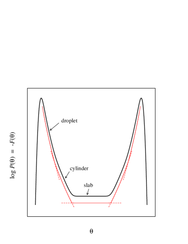
Figure 1: Order parameter probability distribution $P(\theta)$ at the transition point $m_{c}^{2}$ in a cubic box with periodic boundary conditions. Thick line: A schematic plot of the distribution on a large but finite volume. Thin line: “thin wall” approximation, consisting of droplet, cylinder and slab topologies.

These are shown with the thin lines in Fig. 1. Note that the change in geometry is by no means continuous: for instance, the change from a droplet into a cylinder at $X=4\pi/81$ must occur via a deformation which increases the area substantially. This causes an energy barrier between different mixed phase topologies, and the topology sectors have overlapping metastability branches.

What happens to the probability distribution when we lower $m^{2}$ slightly from the transition value $m_{c}^{2}$? Now the free energy densities in the symmetric and broken phases are different:

$$\Delta f=f_{\rm symm.}-f_{\rm broken}\simeq\delta m^{2}\times\left[{\frac{df_{\rm symm.}}{dm^{2}}}-{\frac{df_{\rm broken}}{dm^{2}}}\right]_{m^{2}=m_{c}^{2}}=\delta m^{2}{\ell}\,,$$ (2.2)

where $\delta m^{2}=m_{c}^{2}-m^{2}$ and ${\ell}$ is proportional to the “latent heat” of the transition (remember that $m^{2}$ is the temperature parameter). Remaining in our simple thin wall approximation, and further assuming that $\sigma$ remains constant as we change $m^{2}$, the free energy of the mixed phase configurations has an additional contribution proportional to the volume:

$$F(X,m^{2})=F(X,m_{c}^{2})+\delta m^{2}{\ell}XL^{3}+\mbox{const.}$$ (2.3)

In particular, the free energy of a broken phase spherical droplet of volume $V_{d}$ and area $A_{d}$ becomes

$$F_{\rm droplet}(X,m^{2})-F_{\rm symm.}=-\delta m^{2}{\ell}V_{d}+\sigma A_{d}=-\delta m^{2}{\ell}XL^{3}+\sigma(36\pi)^{1/3}X^{2/3}L^{2}\,.$$ (2.4)

The droplet free energy has a maximum $F_{c}=16\pi\sigma^{3}/(3(\delta m^{2})^{2}{\ell}^{2})$ at droplet radius $R_{d}=2\sigma/(-\delta m^{2}{\ell})$. This is the critical droplet size and free energy at supercooling $\delta m^{2}$: droplets smaller than this size can continuously reduce their free energy by shrinking, and larger droplets can by growing. The droplet free energy is shown schematically in Fig. 2. In a finite box the droplet volume should not exceed the droplet $\leftrightarrow$ cylinder stability limit $L^{3}4\pi/81\approx 0.155L^{3}$, as otherwise the critical “droplet” is a cylinder and the box size is essential to determining its behavior, which is unphysical if we are interested in the behavior in the thermodynamic limit. Applied to the critical droplet, this implies that the inequality $\delta m^{2}{\ell}>6\sigma/L$ should be satisfied.

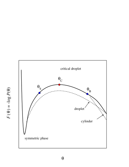
Figure 2: The constrained free energy $F(X)=-\log P(X)$ at a small supercooling $\delta m^{2}$.

Naturally, in a more realistic case the situation is not as simple as in the thin wall case. The phase interfaces have a finite thickness, the shape of the mixed phase domains fluctuates, as also does the value of the order parameter, averaged over the volumes of the pure phase domains. Nevertheless, provided that the volume is sufficiently large, the basic topological structure outlined above remains — even if the shape of the cylinders, droplets and slabs becomes distorted, the magnitude of the fluctuations is restricted by the increase in the free energy (area$\times\sigma$) of the domains. The resulting probability distribution is a “smeared” version of the thin-wall case, with the pure phase $\delta$-peaks rounded into Gaussian distributions. This is shown as thick lines in Figs. 1 and 2.

The probability distribution $P(\theta)$ is to be measured with Monte Carlo simulations. Due to the enormous suppression of the critical droplets, standard Monte Carlo simulations, where configurations are sampled with weight $p\propto\exp[-H]$, are completely inadequate for the task. However, the multicanonical  Monte Carlo method [21] has been developed for just this kind of task; this will discussed in Sec. 4.2. From the measured probability distribution $P(\theta)\propto\exp(-F(\theta))$ at small supercooling $\delta m^{2}$ we can measure the critical droplet free energy

$$F_{C}(\delta m^{2})\approx F(\theta_{C})-F(\theta_{\rm symm.})=-\log{\frac{P(\theta_{C})}{P(\theta_{\rm symm.})}}\,,$$ (2.5)

where $\theta_{C}$ is the local maximum of the free energy, and $\theta_{\rm symm.}$ is the location of the symmetric phase minimum. Since one should remain a safe distance away from the cylinder and slab regions, $X$ should remain well below $\approx 0.15$. This limits the range of $\delta m^{2}$ which can be probed at a given $L$, or sets what $L$ is required for a given $\delta m^{2}$. We note that Eq. (2.5) resembles the widely used histogram method for calculating the planar interface surface tension $\sigma$, proposed by Binder [22]. In some cases Eq. (2.5) can already give a fair estimate of the droplet nucleation rate:

$$\Gamma\propto\mbox{[time]}^{-1}\mbox{[length]}^{-3}\exp(-F_{C})\,,$$ (2.6)

where [time] and [length] are suitably chosen dimensionful constants. Unfortunately, Eq. (2.6) tells us nothing about the constant of proportionality, and the dynamical information is missing completely. The result also explicitly depends on our choice of the order parameter. Thus, the rate can be off by orders of magnitude. Furthermore, as opposed to Binder’s method, which gives the surface tension $\sigma$ exactly as $V\rightarrow\infty$, Eq. (2.5) does not have a well-behaved infinite volume limit with fixed $\delta m^{2}$. The main problem is that, for a fixed supercooling and droplet size, we have $\theta_{C}-\theta_{\rm symm}\propto 1/V$, but the width of the Gaussian-like symmetric phase peak is $\propto 1/V^{1/2}$. Thus, the symmetric phase fluctuations will “swallow” $\theta_{C}$ when the volume is too large! In practice, this does not appear to be a problem for suitably chosen order parameters (see Sec. 4.1).

2.2 Rate of droplet nucleation

Although the droplet nucleation rate is inherently a non-equilibrium problem, in a finite (but large) volume it can be formulated fully in thermal equilibrium. Let us take an ensemble of configurations in thermal equilibrium at small supercooling $\delta m^{2}$, and let each of the configurations evolve according to some dynamical prescription. Naturally, we require that the evolution preserves the equilibrium ensemble, and we consider here only Markovian dynamics which satisfy detailed balance:

$${\frac{T[{(\phi_{a},\pi_{a})\rightarrow(\phi_{b},\pi_{b})}]}{T[{(\phi_{b},{-\pi_{b}})\rightarrow(\phi_{a},{-\pi_{a}})}]}}=\exp[H(\phi_{b},\pi_{b})-H(\phi_{a},\pi_{a})]\,.$$ (2.7)

Here $\phi$ are field variables, $\pi$ the momentum variables (which may not exist in the dynamics at all). $H(\phi,\pi)=H(\phi,-\pi)$ is the energy of the state (scaled by $T$ to be dimensionless), and $T(a\rightarrow b)$ is the transition probability (along some trajectory) from state $a$ to $b$. All standard dynamics we know of obey this condition (for example, Hamiltonian, Langevin, Glauber, heat bath).

We specialize to supercooling, so $m^{2}<m_{c}^{2}$, and at any small time interval the vast majority of the configurations remain in the broken phase, a much smaller fraction are in the symmetric phase, and a tiny number of configurations are in the process of evolving from one phase into another. In equilibrium the rate must be equal in both directions. Let us choose two order parameter values $\theta_{S}$ and $\theta_{B}$ on the symmetric and broken phase sides of $\theta_{C}$, chosen so that the constrained free energy $F(\theta_{S}),\,F(\theta_{B})\ll F(\theta_{C})$; see Fig. 2. If we now take a configuration from the thermal distribution with order parameter restricted to $\theta_{S}$ and let it evolve in time, due to the steep slope in the free energy, it is almost certain not to evolve to $\theta_{C}$ in the “medium term,” i.e. in timescales shorter than the very long tunneling time $1/\Gamma V$. Similarly, a configuration at $\theta_{B}$ is overwhelmingly more likely to fall down into the broken phase than to go to the critical droplet.

During the tunneling the configuration must evolve along a continuous trajectory through the order parameter values $\theta_{S}\rightarrow\theta_{C}\rightarrow\theta_{B}$. We shall focus on the piece of the real time evolution trajectory between the last time the order parameter had the value $\theta_{S}$, before reaching $\theta_{B}$ for the first time. Since the time evolution of the order parameter may be “noisy,” this trajectory may cross the value $\theta_{C}$ several times in a short time interval. We note here that the values of $\theta_{S}$ and $\theta_{B}$ are not critical, as long as the free energy condition $F(\theta_{S,B})\ll F(\theta_{C})$ is satisfied. For example, we could choose $\theta_{S}$ to be well within the bulk of the symmetric phase; the point is that the trajectory $\theta_{S}\rightarrow\theta_{B}$ can be used to identify the tunneling events.

We define the symmetric phase probability $P_{\rm symm.}$ to be the integral of the canonical distribution $P(\theta)\propto\log[-F(\theta)]$ up to up to the critical droplet value $\theta_{C}$,

$$P_{\rm symm.}=\int_{\theta_{\rm min}}^{\theta_{C}}d\theta P(\theta)\,,$$ (2.8)

with $\theta_{\rm min}$ the smallest possible value of $\theta$. The choice of $\theta_{C}$ here is for convenience; since by far the dominant contribution to the integral comes from the central peak of the symmetric phase, choosing some other reasonable value in the neighborhood of $\theta_{C}$ would give only exponentially suppressed corrections.

Let $n_{s}(t)$ be the probability that a configuration which was in the symmetric phase at time $t=0$ still remains there at time $t$, normalized so that $n_{s}(t=0)=P_{s}$. The tunneling rate $\Gamma$ is defined through

$$\Gamma Vn_{s}(t)=-{\frac{dn_{s}(t)}{dt}}\hskip 28.45274pt\rightarrow\hskip 28.45274ptn_{s}(t)=n_{s}(0)\exp\left[-\Gamma Vt\right]\,.$$ (2.9)

This immediately suggests that we can measure $\Gamma$ by simply measuring the average time $\tau$ it takes for the symmetric phase configurations to tunnel: $\Gamma=1/(V\tau)$. However, when the rate is very small, as it is in our case, this approach is utterly impractical.

Let us now consider times which are much shorter than the tunneling time, $t\ll 1/(V\Gamma)$ (this will not restrict the validity of the final results). In this case the symmetric phase consists almost entirely of configurations which were there already at $t=0$. We can substitute $n_{s}(t)\approx n_{s}(0)=P_{s}$ on the l.h.s. of Eq. (2.9), and $dn_{s}(t)/dt$ becomes the time-independent flux of configurations from the symmetric to the broken phase. The central idea of the method described here is the realization that, since all of the tunneling trajectories must go through $\theta_{C}$, we can calculate the flux $dn_{s}/dt$ by sampling configurations and trajectories directly at $\theta=\theta_{C}$. Labelling the configurations with symbol $\phi$ and the trajectories through $\phi$ with $\alpha_{\phi}$, the flux can be written as

$${\frac{dn_{s}}{dt}}=\int d\phi d\alpha_{\phi}\;Ae^{-H(\phi,\alpha_{\phi})}\;\delta(\theta(\phi)-\theta_{C})\,\times{\frac{d\theta(\alpha_{\phi})}{dt}}\times\delta^{\alpha}_{S\rightarrow B}$$ (2.10)

Here $A\exp{-H(\phi,\alpha_{\phi})}$ gives the thermal equilibrium probability of a configuration $\phi$ and a trajectory $\alpha_{\phi}$ which goes through it. In other words, we want to average over all configurations $\phi$ such that $\theta(\phi)=\theta_{C}$, and all trajectories which go through the configuration $\phi$, with the correct, thermal weight. $A$ is a normalization constant, which satisfies

$$\int d\phi d\alpha_{\phi}Ae^{-H(\phi,\alpha_{\phi})}\delta(\theta(\phi)-\theta)=P(\theta),$$ (2.11)

where $P(\theta)$ is the order parameter probability distribution.

The dynamical information is contained in the last two terms of the integrand in Eq. (2.10). The derivative $d\theta(\alpha_{\phi})/dt$ is evaluated along the trajectory $\alpha_{\phi}$ at the point where $\alpha_{\phi}$ crosses the pivot configuration $\phi$. Its purpose is to cancel the Jacobian factor arising from the $\delta$-function: along the trajectory,

$$\delta(\theta-\theta_{C})=\left|{\frac{d\theta}{dt}}\right|^{-1}\delta(t-t_{C}),$$ (2.12)

where $t_{C}$ is the time when the configuration crosses the point $\theta_{C}$. Thus, it turns the integrand from a probability density of configurations at $\theta_{C}$ to a flux of trajectories through the value $\theta_{C}$. This can be understood in another way: if $d\theta/dt$ is small for trajectory $\alpha$, a configuration evolving along it loiters near $\theta_{C}$ longer than a configuration on a trajectory where $d\theta/dt$ is large. Thus, a “slow” trajectory contributes more to the probability density $e^{-H}\delta(\theta-\theta_{C})$ than a “fast” one; and the inclusion of $d\theta(\alpha)/dt$ exactly cancels this bias.

Finally, in order to count only trajectories which really tunnel from the symmetric phase to the broken phase, we define the projection $\delta_{S\rightarrow B}^{\alpha}=1$, if $\alpha$ tunnels from $\theta_{S}$ to $\theta_{B}$; $\delta_{S\rightarrow B}^{\alpha}=0$ otherwise. As discussed above, we define the tunneling trajectories to be ones which evolve from $\theta_{S}$ through the configuration $\phi$ to $\theta_{B}$. The result is that the integral in Eq. (2.10) evaluates the number density  of tunneling trajectories through $\theta_{C}$, which is exactly the rate we are after.

During the evolution from $\theta_{S}$ to $\theta_{B}$ the tunneling trajectories may cross $\theta_{C}$ several times (always an odd number), and these trajectories are counted by the integral (2.10) at every crossing. There is no overcounting, however: if there are $(2n{+}1)$ crossings, in $(n{+}1)$ of these $d\theta/dt$ is positive, and in $(n)$ it is negative, corresponding to crossings left$\rightarrow$right and right$\rightarrow$left, respectively. The absolute magnitude of the integrand is equal at every crossing of $\phi^{2}_{{\rm av},C}$ along the trajectory: it follows from Eqs. (2.7), (2.10) and Eq. (2.12) that the probability of choosing a crossing configuration $\phi_{a}$ and a trajectory which evolves to another crossing configuration $\phi_{a}\rightarrow\phi_{b}$, is equal to choosing one evolving $\phi_{b}\rightarrow\phi_{a}$. Thus, $n$ positive and negative contributions cancel, and the trajectory is counted only once.

This also implies that the dynamical factors in Eq. (2.10) can be rewritten in the following form, which is much more suitable for numerical work:

$${\frac{d\theta(\alpha)}{dt}}\times\delta^{\alpha}_{S\rightarrow B}\,\longrightarrow{\frac{1}{2}}\bigg{|}{\frac{d\theta(\alpha)}{dt}}\bigg{|}\times{\frac{\delta^{\alpha}_{\rm tunnel}}{N^{\alpha}_{\rm crossings}}}\,.$$ (2.13)

Here $N^{\alpha}_{\rm crossing}$ is the number of times the trajectory $\alpha$ crosses $\theta_{C}$, and $\delta^{\alpha}_{\rm tunnel}=1$ for trajectories which tunnel either $\theta_{S}\rightarrow\theta_{B}$ or $\theta_{B}\rightarrow\theta_{S}$: since the whole ensemble is in thermal equilibrium, the flux of trajectories from the symmetric to the broken phase must equal the inverse one. We can take an average over the two sets of trajectories, hence the factor $1/2$ in (2.13). Using the expression (2.13) makes the integrand in Eq. (2.10) positive definite, which improves the convergence of the numerical Monte Carlo integration.

In Eq. (2.10) we implicitly assumed that the trajectory is differentiable in $t$. This is true for Hamiltonian type dynamics, but not for “noisy” time evolution, like Langevin or Glauber dynamics. In these cases we must substitute the derivative with a finite difference:

$${\frac{d\theta}{dt}}\rightarrow{\frac{\Delta\theta}{\Delta t}}\,,$$ (2.14)

and the trajectory must be sampled with the same frequency $\Delta t$ when the crossings in Eq. (2.13) are counted. Due to the noisiness of $\theta(t)$, the smaller $\Delta t$ is, the more crossings of $\theta_{C}$ are potentially resolved. However, this is compensated by the increase in $\Delta\theta/\Delta t$. For example, in Langevin dynamics, when $\Delta t$ is small enough, the trajectory $\theta(t)$ behaves almost like a Brownian random walk in the proximity of $\theta_{C}$. In this case $\langle|\Delta\theta/\Delta t|\rangle\sim(\Delta t)^{-1/2}$, and $\langle N_{\rm crossings}\rangle\sim(\Delta t)^{-1/2}$. Thus, neither of these terms have a $\Delta t\rightarrow 0$ limit, but the product in Eq. (2.13) has.

The use of finite time differences arises automatically in numerical time evolution, also in Hamiltonian evolution, and we shall use this formulation from now on. It is natural to use the same $\Delta t$ in sampling the trajectory as is the step size of the time evolution; however, this is not necessary and the sampling interval can be longer. However, it should not be so long that the free energy $F(\theta)$ changes appreciably in one interval. In practice this is not a problem.

2.3 Monte Carlo evaluation

In practical Monte Carlo simulations we evaluate Eq. (2.10) as follows: let us select configurations from the thermal ensemble, $p\propto e^{-H}$, but with the order parameter restricted to a narrow range $|\theta-\theta_{C}|<\epsilon/2$. We can now construct trajectories (one or more for each configuration) going through $\phi$ by evolving the configuration both forward and backwards  in time, until both the forward and the backwards ends of the trajectory reach order parameter values $\theta_{S}$ or $\theta_{B}$. The trajectory contributes to tunneling only if the ends of the trajectory are on different sides of $\theta_{C}$. Thus, the Monte Carlo version of Eq. (2.10) becomes

$$\Gamma V=P_{C}^{\epsilon}\,{\frac{1}{2}}\left\langle\bigg{|}{\frac{\Delta\theta(\alpha)}{\Delta t}}\bigg{|}\times{\bf d}^{\alpha}\right\rangle\,,$$ (2.15)

where we have defined ${\bf d}^{\alpha}=\delta_{\rm tunnel}^{\alpha}/N^{\alpha}_{\rm crossings}$, and

$$P_{C}^{\epsilon}={\frac{1}{\epsilon P_{\rm symm.}}}\,\int_{\theta_{C}-{\frac{\epsilon}{2}}}^{\theta_{C}+{\frac{\epsilon}{2}}}P(\theta)d\theta\,.$$ (2.16)

Here we have substituted the $\delta(\theta-\theta_{C})$-function in Eq. (2.10) with a small but finite width $\epsilon$; in practice, it is much easier to generate configurations in this ensemble than with a sharp $\delta$-function. The derivative $d\theta/dt$ is again evaluated at the initial configuration $\phi$, and the expectation value $\langle\cdot\rangle$ is over the configurations and trajectories.

The evolution backwards in time means that we invert the (possible) initial momenta $\pi\rightarrow-\pi$ and evolve the system using the standard equations of motion; the time is just interpreted as $-t$. If the dynamics does not involve momenta (for example Langevin or Glauber), then the evolution backwards is just another realization of the standard forward evolution. The detailed balance condition (2.7) guarantees that the trajectory generated by this backwards evolution can be re-interpreted as a representative forward evolving trajectory.

The expression (2.15) is straightforward to use in simulations. However, we simplify it here a bit further: for the physical process we are considering in this work, it turns out that $|\Delta\theta(\alpha)/\Delta t|$ is almost completely uncorrelated with the “global” properties of the trajectory $\alpha$, that is, how many crossings of $\theta_{C}$ it makes, or whether it finally contributes to tunneling. This implies that to good approximation we can evaluate the expectation values of the two terms inside the angle brackets separately:

$$\Gamma V\simeq P_{C}^{\epsilon}{\frac{1}{2}}\left\langle\bigg{|}{\frac{\Delta\theta}{\Delta t}}\bigg{|}\right\rangle\,\left\langle{\bf d}\right\rangle\,.$$ (2.17)

Both of the expectation values above are thermal averages over all trajectories which go through $\theta_{C}$. This is the form of the rate equation given in Ref. [19]. The advantage here is that $\langle|\Delta\theta/\Delta t|\rangle$ is a ‘local’ quantity, and its evaluation does not require the full knowledge of the trajectory. Indeed, for the cubic anisotropy model, with the order parameter and the real-time dynamics we shall consider in this work, it is possible to evaluate it analytically, see Sec. 5.2. The decomposition of the expectation value in (2.17) is a natural consequence of the fact that the critical droplets are large objects, and thus must involve a large number of microscopic variables. The evolution of the UV-modes of these variables is largely uncorrelated across the droplet. The decomposition holds strictly in the zero lattice spacing limit, where $|d\phi^{2}_{\rm av}/dt|$ is UV dominated. However, if one applies the method described here to tunneling processes where only relatively few microscopic degrees of freedom participate, one cannot rely on the decomposition and the equation (2.15) must be used instead.

2.4 Independence on the order parameter

In the discussion above we made extensive use of the critical droplet order parameter value $\theta_{C}$, where the free energy $F(\theta)$ has a local maximum. However, we could have used any other value of $\theta$ in the neighborhood of the free energy maximum — we only have to make sure that the whole of the bulk of the symmetric phase probability remains on the symmetric phase side of it. Intuitively this is clear. What Eq. (2.10) actually measures is the number of trajectories going from $\theta_{S}$ to $\theta_{B}$; and this must be the same, no matter what point in between we decide to intercept them. For example, we may choose a new value $\theta^{\prime}$, somewhat to the symmetric phase side of $\theta_{C}$, to be our new starting point. The probability factors in the integrals (2.10) or (2.15) increase (the free energy is lower), but this is exactly compensated for by the decrease in the average value of the projection $\delta_{\rm tunnel}^{\alpha}$: most of the trajectories which intersect $\theta^{\prime}$ will both start and end in the symmetric phase and hence do not contribute to the tunneling. However, if we want to get as accurate a result as possible for a given amount of cpu-time, it pays to choose the starting value as close to $\theta_{C}$ as possible.

Very significantly, the rate calculated with (2.10)–(2.17) is independent of the choice of the order parameter itself. This is in contrast to the probability distribution $P(\theta)$ alone (which can be used to calculate the free energy of the critical droplet, see Sec. 2.1). The requirement the order parameter has to fulfill is that it separates the symmetric and broken phases and resolves the potential barrier between them to a sufficient degree, in order for one to be able to choose the points corresponding to $\theta_{S}$, $\theta_{C}$ and $\theta_{B}$. Provided that the hierarchy in free energies $F(\theta_{C})\gg F(\theta_{S}),F(\theta_{B})$ is satisfied, the order parameters yield equal results, up to exponentially suppressed corrections, of order $\exp[(F(\theta_{S})-F(\theta_{C}))]\ll 1$.

However, not all order parameters are created equal: the best parameter has as small fluctuations in the bulk phases as possible, while separating the two phases as strongly as possible. Large fluctuations will reduce the resolving power of the order parameter: for example, we may have a droplet which is slightly smaller than the true critical droplet, but a fluctuation in the bulk may still bring the order parameter up to $\theta_{C}$. These fluctuations will typically increase the probability $P(\theta_{C})$, and again, this increase is exactly cancelled by a decrease in $\delta_{\rm tunnel}^{\alpha}$: the trajectories evaluated from these configurations are less likely to lead to tunneling. Thus, the better the order parameter, the larger the fraction of trajectories which lead to tunneling. Especially important is that the fluctuations of the order parameter in the symmetric phase should be very small, since more than 85% of the lattice volume in a critical droplet configuration will remain in the symmetric phase, outside the droplet.

3 Cubic anisotropy model

For concrete calculations in this work we use the cubic anisotropy model in 3 dimensions. The reasons for choosing this are the following: (1) it has a radiatively generated first order phase transition, the strength of which can be adjusted continuously; (2) it is a (superficially) simple model and relatively easy to study on the lattice; (3) it is a continuum field theory, and we can test whether our nucleation calculation gives consistent results as the continuum limit is taken on the lattice. Furthermore, recently the validity of Langer’s theory of nucleation has been questioned in radiatively generated transitions, using exactly this model as an example [14].

3.1 Definition of the model

The cubic anisotropy model is a model with two scalar fields $\phi_{1}$ and $\phi_{2}$, with quartic interactions respecting the discrete symmetries $\phi_{1}\leftrightarrow\phi_{2}$ and $\phi_{1}\leftrightarrow-\phi_{1}$. The thermodynamics of the model is defined by the partition function (We use here “particle physics” units where [length] = [time] = [energy]^-1 = [temperature]^-1),

$$Z=\int{\cal D}\phi_{1}{\cal D}\phi_{2}\,\exp-H_{0}[\phi]\,,$$ (3.1)

where the 3-dimensional action is

$$H_{0}[\phi]=\int d^{3}x\left[\sum_{a=1,2}\left({\frac{1}{2}}\sum_{i=1}^{3}(\partial_{i}\phi_{a})^{2}+{\frac{m^{2}}{2}}\phi_{a}^{2}+{\frac{\lambda_{1}}{24}}\phi_{a}^{4}\right)+{\frac{\lambda_{2}}{4}}\phi_{1}^{2}\phi_{2}^{2}\right]\,.$$ (3.2)

The scalar fields $\phi_{1},\phi_{2}$ have dimensions of $\mbox{(length)}^{-1/2}$, and the coupling constants $\lambda\sim\mbox{(length)}^{-1}$. In the case that the 3 dimensional theory arises from dimensional reduction of a 3+1 dimensional, relativistic scalar field theory, the 3-D quantities are related to the 3+1 dimensional quantities through $H_{0}=H_{\rm 4D}/T$, $\phi=\phi_{\rm 4D}T^{1/2}$, $\lambda=\lambda_{\rm 4D}T$, and $m^{2}=m^{2}_{\rm 4D}+O(T^{2})$. Besides rescaling the 3 dimensional parameters, changing the temperature of the 3+1 dimensional system adjusts the value of $m^{2}$, which is why we often equate lowering $m^{2}$ with cooling.

The mass parameter $m^{2}$ drives the transition: when $m^{2}$ has a large enough positive value, the system is in the symmetric phase $\langle\phi_{1}\rangle=\langle\phi_{2}\rangle=0$, whereas with large and negative $m^{2}$ we are in the broken phase where $|\langle\phi_{1}\rangle|+|\langle\phi_{2}\rangle|>0$. At the mean field level (“tree level” in particle physics parlance) the transition between the symmetric and broken phases is of second order and happens at $m^{2}=0$. Also at the mean field level, the stability of the theory requires $\lambda_{1}>0$ and $\lambda_{2}>-\lambda_{1}/3$. We can immediately recognize some special values for the couplings $(\lambda_{1},\lambda_{2})$: first, when $\lambda_{2}=\lambda_{1}/3$, the 4th order term in the energy functional becomes $(\lambda_{1}/24)(\phi_{1}^{2}+\phi_{2}^{2})^{2}$. Thus, the theory has then an O(2) symmetry under rotations of the fields $(\phi_{1},\phi_{2})$, and as we vary $m^{2}$, there is a second order O(2) phase transition. Another special point is $\lambda_{2}=0$, where we have two uncoupled $\phi^{4}$ models. Now the transition is again of second order, of Ising model universality. We also note that the redefinition of the fields

$$(\phi_{1},\phi_{2})\rightarrow{\frac{1}{\sqrt{2}}}(\phi_{1}+\phi_{2},\phi_{1}-\phi_{2})$$ (3.3)

maps Eq. (3.2) onto itself, with

$$m^{2}\rightarrow m^{2},~{}~{}~{}\lambda_{1}\rightarrow{\frac{1}{2}}(\lambda_{1}+3\lambda_{2}),~{}~{}~{}\lambda_{2}\rightarrow{\frac{1}{2}}(\lambda_{1}-\lambda_{2})\,.$$ (3.4)

The O(2) invariant point $\lambda_{2}=\lambda_{1}/3$ is a fixed point of this transformation, and the region $\lambda_{2}>\lambda_{1}/3$ is mapped on $\lambda_{2}<\lambda_{1}/3$. This implies that the point $\lambda_{1}=\lambda_{2}$ is equivalent to $\lambda_{2}=0$, and it too corresponds to two uncoupled $\phi^{4}$ theories with Ising universality.

The behavior of the system at general values of the couplings has been studied by renormalization group methods by Rudnick [11] and Arnold and Yaffe [12]. Their analysis indicates the following behavior:

1. If $0<\lambda_{2}<\lambda_{1}$, the theory will flow to the O(2) fixed point at large distances, and so will have a second order transition with O(2) criticality. In the broken phase there is a Goldstone mode, corresponding to rotations of the $(\phi_{1},\phi_{2})$-vector.

2. If $\lambda_{2}=0$ or $\lambda_{2}=\lambda_{1}$, we have two uncoupled $\phi^{4}$ theories, and the transition is of Ising type.

3. If $\lambda_{2}<0$ or $\lambda_{2}>\lambda_{1}$, the theory does not flow to any weakly coupled infrared stable fixed point, and so might be expected to have a first order phase transition. This is indeed the case, as shown by perturbative analysis [11, 12] and lattice simulations [13].

The first order transition in the last case is generated by radiative effects; in order to observe it perturbatively, one must consider the first loop correction (Coleman-Weinberg effect [23]). Using the $\epsilon$ expansion around $d=4-\epsilon$ dimensions, Arnold and Yaffe [12] calculated the effective potential up to next-to-next-to-leading order in $\epsilon$. In the limit $\lambda_{2}\gg\lambda_{1}$, the transition becomes strong and the perturbative analysis should be accurate. There are 4 degenerate broken phases in the region of the first order phase transition. If we choose $\lambda_{2}>\lambda_{1}$, in the broken phase the $(\phi_{1},\phi_{2})$ -doublet acquires an expectation value along one of the principal axes: $(\pm v,0)$ or $(0,\pm v)$.

In this work we are interested in strong first order transitions. Thus, we choose $\lambda_{2}=8\lambda_{1}$, which is seen to give a very strong transition.

3.2 Cubic anisotropy model on the lattice

We discretize the theory on the lattice using an ${\mathcal{O}}(a^{2})$ accurate lattice action, where $a$ is the lattice spacing. The action can be written as

$$H_{0} = \sum_{x}\Bigg{[}\frac{Z_{\phi}}{2}\left(-\phi_{1}\nabla^{2}_{\rm L}\phi_{1}-\phi_{2}\nabla^{2}_{\rm L}\phi_{2}\right)+\frac{Z_{m}(m^{2}+\delta m^{2})}{2}\left(\phi_{1}^{2}+\phi_{2}^{2}\right)+$$ (3.5)

$$\qquad+\frac{(\lambda_{1}+\delta\lambda_{1})}{24}\left(\phi_{1}^{4}+\phi_{2}^{4}\right)+\frac{(\lambda_{2}+\delta\lambda_{2})}{4}\phi_{1}^{2}\phi_{2}^{2}\Bigg{]}\,,$$

where we have rescaled the lattice fields and couplings to be dimensionless: $\phi_{\rm latt.}=\phi_{\rm cont.}a^{1/2}$, $\lambda_{\rm latt.}=\lambda_{\rm cont.}a$, and $m^{2}_{\rm latt.}=m^{2}_{\rm cont}a^{2}$. $\delta$-terms and $Z$-factors are additive and multiplicative renormalization constants, respectively. They are necessary to match the behavior of the lattice theory to the continuum theory without $O(a^{2})$ errors, and their calculation is detailed in the appendix. Eliminating such errors also requires a lattice Laplacian which includes next-neighbor couplings,

$$\nabla^{2}_{\rm L}\phi(x)=-\frac{15}{2}\phi(x)+\frac{4}{3}\sum_{i}\Big{(}\phi(x+i)+\phi(x-i)\Big{)}-\frac{1}{12}\sum_{i}\Big{(}\phi(x+2i)+\phi(x-2i)\Big{)}\,.$$ (3.6)

Furthermore, the operator insertion $\langle\phi^{2}\rangle=\langle\phi_{1}^{2}+\phi_{2}^{2}\rangle$, which we will need in what follows, is additively and multiplicatively corrected,

$$a\langle\phi^{2}\rangle_{\rm contin}=Z_{m}\langle\phi^{2}\rangle_{\rm latt}-\delta\langle\phi^{2}\rangle\,.$$ (3.7)

3.3 Real time dynamics

To define the nucleation rate , we must specify a dynamical prescription for the time evolution. The rate will depend on the choice, which, after all, determines what physical system we are describing. Any prescription which preserves the canonical distribution is permitted. The most common evolution prescriptions in field theories are the Hamiltonian and the Langevin dynamics. Both are perfectly valid evolution dynamics for classical thermal field theories; for our case the Hamiltonian dynamics has the further conceptual advantage that it also describes the evolution of a quantum theory at high temperatures to leading order in coupling constants [24, 25].

In this work we shall consider a one-parameter class of evolution dynamics, the Hamiltonian stochastic equations  [26, 27]

$$\partial_{t}\phi_{a}(x,t) = \pi_{a}(x,t)$$

$$\partial_{t}\pi_{a}(x,t) = -{\frac{\delta H_{0}}{\delta\phi_{a}}}+\gamma\pi_{a}(x,t)+\xi_{a}(x,t)\,.$$ (3.8)

Here $H_{0}$ is given by Eq. (3.2), $\pi_{a}$ are the momentum variables of fields $\phi_{a}$, $\gamma\geq 0$ is a “friction coefficient,” and $\xi_{a}(x,t)$ is Gaussian noise, which satisfies the stochastic condition

$$\langle\xi_{a}(x,t)\xi_{b}(x^{\prime},t^{\prime})\rangle=2\gamma\delta_{ab}\delta^{3}(x-x^{\prime})\delta(t-t^{\prime})\,.$$ (3.9)

The equations of motion (3.8) thermalize the system (if $\gamma>0$), that is, at large times the probability distribution approaches the Gibbs distribution $p\propto\exp(-H[\phi,\pi])$, where

$$H[\phi,\pi]=\int d^{3}x{\frac{1}{2}}(\pi_{1}^{2}+\pi_{2}^{2})+S_{0}[\phi]\,.$$ (3.10)

Thus, the evolution also preserves the correct thermodynamics of the “static” theory, Eq. (3.1).

If we choose $\gamma=0$ in Eqs. (3.8) the evolution becomes the standard canonical Hamiltonian evolution, with canonical momenta $\pi_{a}$ and conserved energy $H$. On the other hand, if $\gamma$ is very large, the equations of motion can be reduced to the familiar fully diffusive Langevin equation for $\phi$, simply by eliminating $\pi$ and neglecting the term (small in this limit) $\partial_{t}^{2}\phi$. Thus, by adjusting $\gamma$ we can continuously adjust the coupling of the system to an external “heat bath.”

For the case of droplet nucleation at finite volume the presence of noise improves the finite volume and lattice spacing scaling of the dynamics. This is because the transition has a large latent heat. A growing/shrinking droplet will release/absorb a significant amount of energy. Under microcanonical Hamiltonian dynamics the temperature in a finite system will correspondingly increase/decrease. In an infinite volume, the released energy would be transported rapidly away from the proximity of the droplet by hydrodynamical flows, and the temperature would remain close to constant. As the lattice spacing becomes smaller, the heat capacity of the system grows, and the latent heat again becomes less important. But at finite lattice spacing and volume, the latent heat remains indefinitely under Hamiltonian dynamics, modifying the time development. A finite $\gamma$ in Eqs. (3.8) absorbs the latent heat, allowing the system to more rapidly approach the infinite volume behavior. It does this efficiently for $\gamma\mathop{\raise 1.29167pt\hbox{$>$\kern-7.5pt\raise-4.73611pt\hbox{$\sim$}}}1/L$, in which case the momenta thermalize completely in time $\tau\mathop{\raise 1.29167pt\hbox{$<$\kern-7.5pt\raise-4.73611pt\hbox{$\sim$}}}L$. In Sec. 5 we check the dependence of the nucleation rate on $\gamma$, and we find that we can vary $\gamma$ over a large range without significantly affecting the results. This means that, in practice, the nucleation rate has a fairly weak dependence on the specifics of the real time dynamics.

3.4 Real time evolution on the lattice

The discretization of the equations of motion (3.8) requires some care, because certain errors lead to time evolution which respects a slightly different ensemble of configurations than the Gibbs one. This is important, because slight thermodynamic changes dramatically affect the critical bubble behavior. The easiest safe update at nonzero $\gamma$ is to apply Hamiltonian evolution, stopping every $\Delta t\ll a$ to apply a partial momentum refresh,

$$\pi_{a}(x,t+0)=(1-\varepsilon^{2})^{1/2}\,\pi_{a}(x,t-0)+\varepsilon\eta_{a}(x,t)\,,$$ (3.11)

with $\epsilon^{2}=\left(1-\exp(-2\gamma\Delta t)\right)$. This refresh exactly preserves the Gibbs distribution. We perform $\Delta t$ of Hamiltonian evolution by a single step of the fourth order Runge-Kutta algorithm [29], which has errors suppressed by $(\Delta t/a)^{5}$. This procedure reproduces Eq. (3.8) with errors of order $O([\Delta t/a]^{2})$, $O(\epsilon^{2})$, but what is more important, it maintains the Gibbs distribution to $O([\Delta t/a]^{4})$ errors. We use $\Delta t/a=0.05$, which proves more than adequate, unless we want to study extremely large $\gamma$.

4 Numerics and thermodynamic results

4.1 Order parameter

The cubic anisotropy model has a true order parameter, which measures the breaking of the global symmetry:

$$\phi_{\rm av}=\sqrt{(\overline{\phi}_{1})^{2}+(\overline{\phi}_{2})^{2}}\,,\qquad\overline{\phi}_{1}=\frac{1}{N^{3}}\sum_{x}\phi_{1}\,.$$ (4.1)

Here $N^{3}$ is the volume in lattice units. However, a better observable for our purposes is

$$\phi^{2}_{\rm av}={\frac{1}{N^{3}}}\sum_{x}(\phi^{2}_{1}+\phi^{2}_{2})\,.$$ (4.2)

This is clearly not an order parameter in the sense that it would be zero in one phase and non-zero in another. However, it has different expectation values in the symmetric and broken phases, which is sufficient for our purposes. The reasons why we prefer $\phi^{2}_{\rm av}$ over $\phi_{\rm av}$ are that (a) it is much more economical to use, and (b) it resolves the critical droplet more accurately.

Let us first consider the cost. Note that $\phi^{2}_{\rm av}$ is multiplied by $m^{2}$ in the Hamiltonian (3.2). Assuming that we have measured the order parameter distribution at $m^{2}=m_{1}^{2}$,

$$P_{m_{1}^{2}}(\phi^{2}_{\rm av})\propto\int d\phi^{\prime}\exp[-H_{m_{1}^{2}}(\phi^{\prime})]\,\delta(\phi^{\prime\,2}_{\rm av}-\phi^{2}_{\rm av})\,,$$ (4.3)

we obtain the distribution at any other $m_{2}^{2}$ simply by reweighting:

$$P_{m_{2}^{2}}(\phi^{2}_{\rm av})\propto\exp[(m_{1}^{2}-m_{2}^{2})\phi^{2}_{\rm av}]P_{m_{1}^{2}}(\phi^{2}_{\rm av})\,.$$ (4.4)

The reweighting can be done without any significant loss of accuracy: if we have determined $P_{m_{1}^{2}}$ to a good accuracy in some $\phi^{2}_{\rm av}$-range of interest, reweighting gives $P_{m_{2}^{2}}$ with the same relative error $\delta P(\phi^{2}_{\rm av})/P(\phi^{2}_{\rm av})$ in this range. Since the calculation of $P(\phi^{2}_{\rm av})$ comprises the major part of the total computational effort, it is quite significant that we can perform the measurement once, and use it for all $m^{2}$ values. Of course, separate calculations are still required for different lattice volumes and lattice spacings.

As discussed in Sec. (2.4), in order to be able to resolve the droplet as well as possible, the fluctuations of the order parameter in the symmetric phase should be as small as possible — this is because more than 85% of the volume of the lattice is in the symmetric phase in critical droplet configurations. Here $\phi^{2}_{\rm av}$ is a clear winner over $\phi_{\rm av}$. This can be seen by comparing the (width)² of the symmetric phase distributions, i.e. the susceptibilities:

$$\chi(\phi_{\rm av}) = {\frac{1}{V}}\int d^{3}x\langle\phi_{\rm av}(x)\phi_{\rm av}(0)\rangle={\frac{2}{Vm^{2}}}$$ (4.5)

$$\chi(\phi^{2}_{\rm av}) = {\frac{1}{V}}\int d^{3}x\langle\phi^{2}_{\rm av}(x)\phi^{2}_{\rm av}(0)\rangle_{\rm connected}$$ (4.6)

$$= {\frac{4}{V}}\int{\frac{d^{3}p}{(2\pi)^{3}}}{\frac{1}{(p^{2}+m^{2})^{2}}}={\frac{1}{2\pi Vm}}\,.$$

Here $m^{2}$ is the (mass)² of $\phi$ in the symmetric phase. Since the tree-level transition happens at $m^{2}=0$, the value of $m^{2}$ at the transition must be small, of order $\lambda^{2}$. The relevant quantity at the transition is the width of the symmetric phase distribution compared against the broken phase expectation value; using 1-loop effective potential, see Eq. (6.5), we obtain the relative “figure of merit”

$${\frac{\chi^{1/2}(\phi_{\rm av})/v}{\chi^{1/2}(\phi^{2}_{\rm av})/v^{2}}}\approx 13{\rm\;for\;}\lambda_{2}=8\lambda_{1}\,,$$ (4.7)

where $v=\langle\phi_{\rm av}\rangle$ in the broken phase. Thus, the symmetric phase fluctuations of $\phi_{\rm av}$ are more than 10 times larger than $\phi^{2}_{\rm av}$, when normalized to the broken phase expectation values. Naturally, the final word comes from the lattice simulations, where $\phi_{\rm av}$ is indeed observed to give a $\sim 10$ times wider symmetric phase peak than $\phi^{2}_{\rm av}$. The width of the symmetric peak of the the $\phi_{\rm av}$-distribution is actually larger than the critical droplet value $\phi_{{\rm av},C}$ for the parameters we are using in this work. Thus, $\phi_{{\rm av},C}$ does not have the necessary resolution power, while we can use $\phi^{2}_{\rm av}$ without problems. A higher power of $\phi$, for example, $\phi^{4}_{\rm av}$, might give an even narrower symmetric phase peak on a coarse lattice spacing, but in the continuum it would have a UV divergent susceptibility, unlike $\phi^{2}_{\rm av}$, so taking the continuum limit might prove problematic. Such order parameters also fail the economy criterion.

4.2 Multicanonical method

In order to be able to calculate the droplet nucleation rate, our task now is to determine $P(\phi^{2}_{\rm av})$ in the droplet regime, $X<0.15$. Since the probability density can vary by $\sim\exp(100)$ or more in this range, normal Monte Carlo simulations, where the configurations are sampled with probability $p\propto\exp-H$, are completely out of the question. The multicanonical method [21] was originally developed for just this kind of problems. In multicanonical sampling the configurations are chosen with a modified weight

$$p_{\rm muca}\propto\exp[-H_{m^{2}}+W(\phi^{2}_{\rm av})]\,.$$ (4.8)

$W(\phi^{2}_{\rm av})$ is a weight function, which is carefully chosen so that the probability distribution of $\phi^{2}_{\rm av}$ measured from the multicanonical Monte Carlo simulation, $P_{\rm muca}(\phi^{2}_{\rm av})$, is approximately constant in the range of interest. The canonical distribution is then obtained by reweighting with the weight function:

$$P_{m^{2}}(\phi^{2}_{\rm av})\propto e^{-W(\phi^{2}_{\rm av})}P_{\rm muca}(\phi^{2}_{\rm av}).$$ (4.9)

This can be further reweighted to other values of $m^{2}$ using Eq. (4.4).

An optimal choice for $W$ is $-\log P_{m^{2}}(\phi^{2}_{\rm av})$, which is just the quantity we want to calculate with the multicanonical simulation! The weight function need not be exactly the ideal one, but it must not deviate from it too much or the multicanonical simulation becomes very inefficient. This chicken-and-egg problem can be resolved by first calculating $W$ with an automatic iterative feedback procedure [30, 31]. We use a variation of the one presented in Ref. [30]. This method yields progressively better approximations for $W$, until sufficient accuracy is reached. The final $W$ can then be used in a multicanonical simulation, which finally gives us $P(\phi^{2}_{\rm av})$. A detailed description of the application of the multicanonical method to the problem of the bubble nucleation in the electroweak theory can be found in [19].

In the multicanonical phase of the simulations we are at liberty to choose as efficient an update algorithm as possible. (In the real-time runs the evolution equations fix the update.) We use a mixture of site by site heat bath and a non-local multi-grid over-relaxation.

4.3 Results: thermodynamics

Before tackling the droplet nucleation rate calculation, we want to study basic thermodynamic quantities associated with the phase transition: the transition “temperature” $m^{2}=m_{c}^{2}$, the “latent heat” ${\ell}$, and the tension of the interface between the symmetric and broken phases $\sigma$. We want the above quantities in the true thermodynamic limit, that is, we extrapolate to infinite volume and to zero lattice spacing. All of the simulations have been done with $\lambda_{1}/\lambda_{2}=1/8$, which guarantees a strong first order transition.

In this part of the analysis we use up to 6 different lattice spacings $a\lambda_{2}=1.5$, 2, 2.5, 3, 3.5 and 4 (all dimensionful quantities are given in terms of $\lambda_{2}$). For every lattice spacing we perform simulations using a series of lattice sizes; all in all, we have 64 simulations at different lattice spacings and volumes. Since the transition is strong, all of the simulations described here are multicanonical (see subsec. 4.2), with the weight function optimized for the whole order parameter range from the symmetric to the broken phase.

Figure 3: Reweighting of the probability distribution $P(\phi^{2}_{\rm av})$ to different values of $m^{2}$. The transition value $m_{c}^{2}$ is the one where the symmetric and broken phase peaks have equal volume.

The transition point $m_{c}^{2}$:

We define the transition value of $m^{2}$ to be the value where the two peaks of the probability distribution $P(\phi^{2}_{\rm av})$ have equal weight, i.e. the value where the volumes of the symmetric and broken phase peaks are equal (see Fig. 3). More precisely, the symmetric and broken phase probabilities are the integrals of the distribution to the right and to the left of a separating value between the peaks; since the probability is exponentially suppressed here in sufficiently large volumes, the precise choice of the separation value is exponentially unimportant. For each lattice spacing $a$, we determine the transition point $m_{c}^{2}$ using a series of volumes and extrapolate the results to infinite volume. The extrapolation is linear in $1/V$, as long as the volumes have similar geometry; an example of this at $a=3/\lambda_{2}$ is shown on the left panel of Fig. 4.

The infinite volume points are in turn extrapolated to the continuum limit $a\rightarrow 0$. This is shown on the right panel of Fig. 4. Since we know the additive mass counterterms only to order $O(a^{0})$ (see appendix A), we extrapolate to the continuum limit using an ansatz $c_{0}+c_{1}x+c_{2}x^{2}+c_{3}x^{3}$, where $c_{i}$ are fitted constants and $x=a\lambda_{2}$. The final result is

$$m^{2}_{c}(\mu=\lambda_{2})/\lambda_{2}^{2}=0.0096\pm 0.00022$$ (4.10)

We note that the supercooling $\delta m^{2}$ can be determined much more accurately than $m_{c}^{2}$: in differences of $m^{2}$ the additive counterterms cancel, and the leading errors behave as $O(a^{3})$. At no stage of the nucleation analysis do we need to know the absolute value of $m_{c}^{2}$.

In the fit the coefficients $c_{1}$ and $c_{2}$ are actually consistent with zero, suggesting that the unknown counterterms are small. We also show a fit with these coefficients set to zero.

Figure 4: Transition value of $m^{2}$ extrapolated to infinite volume at $\lambda_{2}a=2$ (left), and to zero lattice spacing (right). The solid line shows a 3rd order polynomial fit, and the dotted line is a fit of form $c_{0}+c_{3}(\lambda_{2}a)^{3}$.

Figure 5: Surface tension $\sigma/\lambda^{2}_{2}$ extrapolated to infinite volume at $\lambda_{2}a=3$ (left), and to zero lattice spacing (right).

The surface tension $\sigma$:

The surface tension is the free energy per unit area of interface. As discussed in Sec. 2.1, when $m^{2}=m_{c}^{2}$ the suppression of the probability in the mixed phase (in large enough volumes) is caused by the existence of phase interfaces. Approximately half-way between the symmetric and broken phases, the mixed phase configurations consist of slabs of symmetric and broken phases, separated by two approximately planar interfaces. Thus, the interface tension $\sigma$ can be obtained from [22]

$$\sigma=-\lim_{V\rightarrow\infty}\,{\frac{1}{2L_{x}L_{y}}}\log{\frac{P_{\rm slab}}{P_{\rm peak}}}\,.$$ (4.11)

Here we have assumed that the interfaces are oriented parallel to $(x,y)$-plane. As for other quantities we have scaled $T$ out of $\sigma$; a more conventional definition is $\sigma_{c}=\sigma T$, so that $\sigma_{c}\times\mbox{area}$ is the free energy of the interface (rather than the scaled free energy we use in this paper). At the “equal weight” point the symmetric and broken phase heights are not usually equal; in this case $P_{\rm peak}$ is the average of the two peaks. However, here we determine $\sigma$ from distributions which have been reweighted to “equal height” $m^{2}$; in our case, the two definitions give completely consistent results.

The extrapolation to infinite volume in Eq. (4.11) can be substantially improved by using finite volume corrections [32, 33]:

$$\sigma a^{2}=\frac{1}{2n_{x}n_{y}}\log{\Big{(}\frac{P_{\rm peak}}{P_{\rm slab}}\Big{)}}+\frac{1}{n_{x}n_{y}}\Big{(}\frac{4}{3}\log{n_{z}}-\frac{1}{2}\log{n_{x}}+\frac{1}{2}G+\textrm{const.}\Big{)}\,.$$ (4.12)

Here $L_{i}=n_{i}a$ and $\sigma_{L}=\sigma a^{2}$ is the tension in lattice units. The function $G$ interpolates between lattice geometries. For cubical volumes $G=\log 3$, while for long cylinders $G=0$. In our analysis we use strongly cylindrical boxes, $L_{z}\gg L_{x}=L_{y}$. This guarantees that the interfaces form along the $(x,y)$ plane, and it also separates the two interfaces much farther than a cube of the same volume. On the left panel of Fig. 5 we show the extrapolation of $\sigma/\lambda^{2}_{2}$ (corrected with Eq. (4.12)) to infinite volume at lattice spacing $\lambda_{2}a=3$. The continuum limit extrapolation is shown on the right panel. Because of our lattice improvement the leading errors are $O(a^{3})$. We obtain a good fit using a third order ansatz $\sigma(a)=\sigma+c_{3}a^{3}$, with the result

$$\sigma/\lambda_{2}^{2}=0.0050\pm 0.0002\,.$$ (4.13)

The latent heat ${\ell}$:

Since $m^{2}$ is our temperature parameter, we define the latent heat using

$${\ell}=\Delta\left({\frac{df}{dm^{2}}}\right)_{m^{2}=m_{c}^{2}}={\frac{1}{2}}(\langle\phi^{2}_{\rm av}\rangle_{\rm broken}-\langle\phi^{2}_{\rm av}\rangle_{\rm symm.})\,.$$ (4.14)

The difference between the symmetric and broken phase expectation values is readily measurable from the distributions like the one in Fig. 3. Our extrapolation procedure is the same as for $\sigma$:

$${\ell}/\lambda_{2}=0.243\pm 0.004\,.$$ (4.15)

5 Results: the nucleation rate

We evaluate the rate of the droplet nucleation using Eq. (2.17). To recap the discussion in Sec. 2, the calculation consists of two separate stages:

(1) the measurement of the probability distribution of the order parameter, $P(\phi^{2}_{\rm av})$, using multicanonical simulations, and

(2) the real-time evolution of the critical droplets, which gives us $\langle|\Delta\phi^{2}_{\rm av}/\Delta t|\rangle$ and $\langle{\bf d}\rangle$.

$a\lambda_{2}$ size/$a^{3}$ evolution at $\delta m^{2}/\lambda_{2}^{2}$ 4.0 $60^{3}$ 0.001156 3.5 $70^{3}$ 3.0 $60^{3}$, $70^{3}$, $80^{3}$ 0.0007–0.00125 2.5 $100^{3}$ 0.00094 2.0 $120^{3}$

Table 1: The lattice spacing and size where the droplet nucleation rate has been calculated. For each lattice the probability distribution $P(\phi^{2}_{\rm av})$ has been calculated once with a multicanonical simulation. The real-time evolution of the critical droplets are calculated using the supercoolings shown on the third column.

The lattice spacings and sizes used are shown in Table 1. For each of the lattices we calculate $P(\phi^{2}_{\rm av})$ once; as explained in Sec. (4.1) and (4.2), the original distribution can be reweighted to different values of supercooling $\delta m^{2}$. On the other hand, the real-time trajectories have to be calculated separately for each supercooling.

5.1 The probability of the critical droplets

In order to fit the droplets comfortably inside the lattice, the lattice volumes have to be substantially larger than the volumes used in Sec. (4.3). However, as discussed in Sec. (2.1), in this case we have to calculate the probability distribution $P(\phi^{2}_{\rm av})$ only in the “droplet branch” of the distribution, $0\leq[\phi^{2}_{\rm av}-\phi^{2}_{{\rm av},{\rm s}}]<0.15\times[\phi^{2}_{{\rm av},{\rm b}}-\phi^{2}_{{\rm av},{\rm s}}]$. This guarantees that the distance of the droplet from its periodic copies is large and we are a safe distance away from the “cylinder” branch of the distribution. Furthermore, the restricted range of $\phi^{2}_{\rm av}$ reduces the computational requirements in multicanonical simulations dramatically, when compared with the full range calculations in Sec. (4.3); using random walk arguments, the reduction factor is $0.15^{2}\sim 0.02$; in practice, the reduction is even stronger than this.

Figure 6: The probability distribution $P(\phi^{2}_{\rm av})$ at various values of supercooling $\delta m^{2}$, measured from $a\lambda_{2}=3$, $80^{3}$ lattice. Here $\phi^{2}_{\rm av}$ is in lattice units, Eq. (3.7). The critical droplet value $\phi^{2}_{{\rm av},C}$ at each $\delta m^{2}$ is defined to be the location of the local minimum of $P(\phi^{2}_{\rm av})$.

In Fig. 6 we show the actual order parameter distributions $P(\phi^{2}_{\rm av})$, measured from the $a\lambda_{2}=3$, $80^{3}$ lattice, and reweighted to supercooling values $\delta m^{2}/\lambda_{2}=0.00077$–0.00122. The larger the supercooling, the smaller the critical droplet, and less suppressed the droplet probability is. We always use lattice  units for $\phi^{2}_{\rm av}$; since this is an “internal” quantity in the expression for the rate (2.17), there is no need to convert it to continuum units.

We calculate the critical droplet free energy through $F_{C}\approx-\ln(P(\phi^{2}_{{\rm av},C})/P(\phi^{2}_{{\rm av},{\rm s}}))$, where $P(\phi^{2}_{{\rm av},{\rm s}})$ is the height of the symmetric phase peak of $P(\phi^{2}_{\rm av})$. Note that this ratio is not $P_{C}^{\epsilon}$, which appears in the rate equation (2.17); we chose to use this ratio because it is dimensionless, whereas the probability factor in (2.17) has dimensions of $[\phi^{2}_{\rm av}]^{-1}$. In Fig. 7 we show $F_{C}$ using $\lambda_{2}a=3$ lattices of volumes $60^{3}$–$80^{3}$. For large values of supercooling $\delta m^{2}$, where the critical droplet is small, we do not observe any significant finite volume effects. However, when $\delta m^{2}$ is smaller, the critical droplet is large and, in small lattices, the droplet feels the proximity of its periodic copies. For our smallest ($60^{3}$) lattice, this decreases the droplet free energy significantly already at modest droplet sizes. The curves shown in Fig. 7 correspond to droplets which are well within the maximum size determined by the 15% rule discussed in Sec. (2.1). This finite size effect is caused by the finite thickness of the droplet wall, and it should vanish exponentially as the lattice size is increased. Indeed, at large lattices we need to go to very large droplets in order to observe any significant finite size effects.

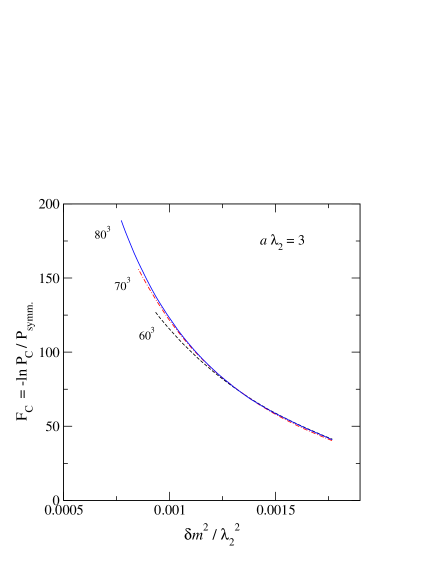
Figure 7: The critical droplet free energy $F_{C}$, as a function of supercooling $\delta m^{2}$, measured from $\lambda_{2}a=3$ lattices of size $60^{3}$–$80^{3}$.

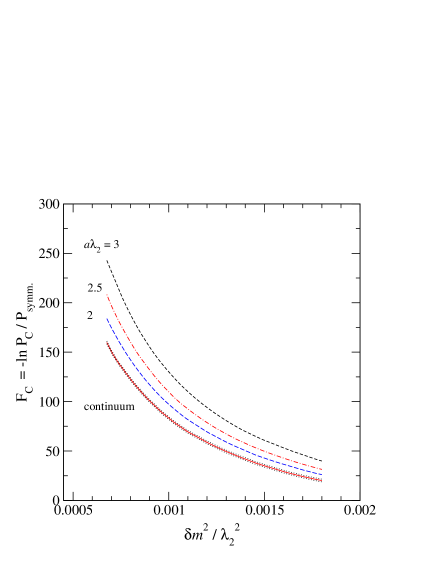
Figure 8: The critical droplet free energies measured from $\lambda_{2}a=3$, volume $80^{3}$; $\lambda_{2}a=2.5$, volume $100^{3}$, and $\lambda_{2}a=2$, volume $120^{3}$ lattices. The continuum ($a=0$) curve is shown with an error band.

On the other hand, the lattice spacing effects are substantial for the values of $a\lambda_{2}$ used: in Fig. 8 we compare $F_{C}$ from lattices of similar physical size, but $a\lambda_{2}=2$, 2.5 and 3. The larger lattice spacings $a\lambda_{2}=3.5$ and 4 have much larger finite $a$ effects and we discard these in our analysis. For a fixed value of supercooling $\delta m^{2}$, $F_{C}$ decreases as the lattice spacing becomes smaller. The leading order errors are expected to be $\mathcal{O}(a^{3})$; indeed, a good fit to the 3 curves is obtained with a 2 parameter fit $c_{0}+c_{3}(a\lambda_{2})^{3}$, done independently for each $\delta m^{2}$. The resulting continuum curve is shown in Fig. 8. The statistical errors in the $F_{C}$ curves are $\approx\pm 0.5$–1.4, and in the continuum extrapolation $\approx\pm 2$; this is shown in the figure.

5.2 Real time evolution (i): $\langle|\Delta\phi^{2}_{\rm av}/\Delta t|\rangle$

The factor $\langle|\Delta\phi^{2}_{\rm av}/\Delta t|\rangle$ is to be evaluated at the critical droplet value $\phi^{2}_{\rm av}=\phi^{2}_{{\rm av},C}$. It is easy enough to measure from numerical simulations, but it can be also calculated analytically: from the equations of motion (3.8) we see that

$${\frac{\Delta\phi^{2}_{\rm av}}{\Delta t}}={\frac{2}{N^{3}}}\sum_{x,a}\pi_{a}\phi_{a}+\mathcal{O}((\Delta t)^{2})\,.$$ (5.1)

Here all the fields and $\Delta t=(\Delta t)_{\rm cont.}/a$ are in dimensionless lattice units. In thermal equilibrium, the momenta $\pi_{a}(x)$ have Gaussian random variable distribution (of width one in our normalization). This implies that $\langle\pi_{a}(x)\pi_{b}(y)\rangle=\delta_{a,b}\delta_{x,y}$, and any expectation values involving products of $\pi$’s and $\phi$’s factorize: $\langle f(\phi)g(\pi)\rangle=\langle f(\phi)\rangle\langle g(\pi)\rangle$. We need to determine $\langle|\Delta\phi^{2}_{\rm av}/\Delta t|\rangle$ at the special value $\phi^{2}_{\rm av}=\phi^{2}_{{\rm av},C}$. Using this constraint, $\sum_{x,a}\phi_{a}^{2}(x)=N^{3}\phi^{2}_{{\rm av},C}$, we obtain

$$\bigg{\langle}\bigg{(}{\frac{\Delta\phi^{2}_{\rm av}}{\Delta t}}\bigg{)}^{2}\bigg{\rangle}_{\phi^{2}_{{\rm av},C}}={\frac{4}{N^{6}}}\sum_{x,a}\langle\phi^{2}_{a}(x)\rangle={\frac{4\phi^{2}_{{\rm av},C}}{N^{3}}}\,.$$ (5.2)

For any fixed $x$ the product $\pi_{a}(x)\phi_{a}(x)$ has a non-Gaussian distribution, but the sum which appears in Eq. (5.1) is Gaussian, due to the global constraint. Because Gaussian distributions satisfy $\langle x^{2}\rangle=\pi\langle|x|\rangle^{2}/2$, we obtain the result

$$\bigg{\langle}\bigg{|}{\frac{\Delta\phi^{2}_{\rm av}}{\Delta t}}\bigg{|}\bigg{\rangle}_{\phi^{2}_{{\rm av},C}}={\frac{1}{a}}\,\sqrt{{\frac{8\phi^{2}_{{\rm av},C}}{\pi N^{3}}}}\,,$$ (5.3)

where we have converted back to continuum time, to remind us of the correct scaling in the continuum limit. Since this result depends only on the average distribution of momenta $\pi$, it is independent of the magnitude of the noise in Eqs. (3.8).

5.3 Real time evolution (ii): $\langle{\bf d}\rangle$

The final contribution to the rate comes from $\langle{\bf d}\rangle=\langle\delta_{\rm tunnel}/{N_{\rm crossings}}\rangle$. This requires the evaluation of full real time trajectories through an ensemble of critical droplets. Following the procedure outlined in Sec. (2.3), we do this as follows:

(1) First, we choose an initial configuration $\phi^{0}_{a}(x)$ from a thermal distribution, but with the order parameter restricted to a narrow interval around the critical droplet value: $|\phi^{2}_{\rm av}-\phi^{2}_{{\rm av},C}|<\epsilon/2$. These are straightforward to generate with either a standard Monte Carlo simulation with the restriction built into the update, or by choosing them from a multicanonical run.

(2) We assign initial momenta $\pi^{0}_{a}(x)$ to this configuration, drawn from a thermal distribution. In our case this means that we choose $\pi_{a}(x)$ from a Gaussian distribution with width $a^{3}\langle\pi^{2}\rangle=1$ (or $\langle\pi^{2}\rangle=1$ in lattice units).

(3) The configuration is then evolved in time until the order parameter $\phi^{2}_{\rm av}$ reaches $\phi^{2}_{{\rm av},S}$ or $\phi^{2}_{{\rm av},B}$, the symmetric or broken phase “cut-off” values. We always use the timestep $\Delta t=0.05a$ in our real time runs. We then return to the initial configuration $\phi^{0}$, invert the initial momenta $\pi^{0}\rightarrow-\pi^{0}$, and evolve the system again until we reach $\phi^{2}_{{\rm av},S}$ or $\phi^{2}_{{\rm av},B}$. This latter run is interpreted as a run backwards in time; by gluing the backwards and forward half-trajectories together at the starting point, we obtain a full trajectory $\phi^{2}_{\rm av}(S{\rm~{}or~{}}B)\rightarrow\phi^{2}_{\rm av}(S{\rm~{}or~{}}B)$. If the trajectory tunnels, i.e. if the backward and forward evolution ends are on different sides of $\phi^{2}_{{\rm av},C}$, it contributes to the tunneling rate ($\delta_{\rm tunnel}=1$). After counting the number of times the trajectory crosses $\phi^{2}_{{\rm av},C}$, we obtain its contribution to $\langle{\bf d}\rangle$.

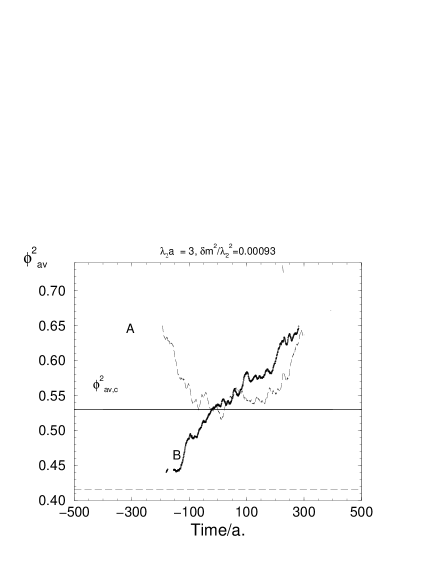
Figure 9: Two trajectories measured from $\lambda_{2}a=3$, $80^{3}$ lattice, at supercooling $\delta m^{2}/\lambda_{2}^{2}=0.00094$ and with noise magnitude $\varepsilon^{2}=2\gamma\Delta t=0.00125$. The trajectories are evaluated forward and backwards in time, starting from configurations at $t=0$. Trajectory A crosses $\phi^{2}_{{\rm av},C}$ 12 times, B 5 times; the contribution to ${\bf d}$ from A is $0/12$, and from B $1/5$. The dashed horizontal line is the symmetric phase expectation value; and $\phi^{2}_{\rm av}$ is shown in lattice units.

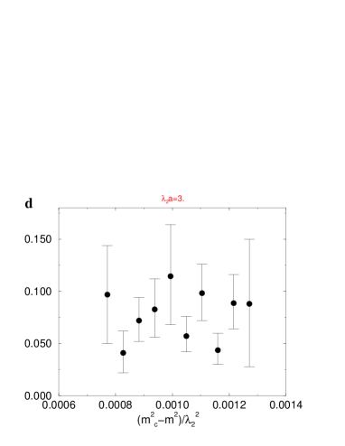
Figure 10: The dynamical factor ${\bf d}$ plotted against $\delta m^{2}$, measured from $a\lambda_{2}=3$, $80^{3}$ lattice.

An example of the trajectories is shown in Fig. 9. About 40% of the trajectories we evaluate are tunneling trajectories. This means that the order parameter resolves the critical droplet quite well, and configurations at $\phi^{2}_{\rm av}=\phi^{2}_{{\rm av},C}$ indeed are a good sample of critical droplet configurations (see the discussion in Sec. 2.4). We measure the order parameter after every timestep. On the scale of the plot the evolution of $\phi^{2}_{\rm av}$ looks rough, but at the level of individual timesteps it is quite smooth. This is due to the relatively small amplitude of the noise in the equations of motion.

In Table 1 we show the lattices and $\delta m^{2}$ values where we evaluate the trajectories. In Fig. 10 we study how ${\bf d}$ depends on the degree of supercooling $\delta m^{2}$. Remember that small values of $\delta m^{2}$ correspond to large critical droplets. At each value of $\delta m^{2}$ we evaluated 35–83 full trajectories. The value of ${\bf d}$ appears to be remarkably stable throughout the range of $\delta m^{2}$ studied; the free energy of the critical droplet varies by $\sim e^{100}$ over this range. Naturally, ${\bf d}$ still depends on $\delta m^{2}$; for example, when $\delta m^{2}\rightarrow 0$ one expects ${\bf d}\rightarrow 0$, simply because the larger the droplet is, the slower it evolves. However, the dependence on $\delta m^{2}$ is not visible within our statistical errors. The large values of the errors are caused by the large variation in the number of crossings between tunneling trajectories: some trajectories have only a few crossings, whereas some have more than 50. The errors of ${\bf d}$ are still sufficiently small for an accurate calculation of the the nucleation rate — since the rate is of order $e^{-100}$, a factor of 2 means little in the final result.

The distribution of the trajectories as a function of the number of crossings appears to decrease roughly exponentially as the number of crossings increases. However, when the number of crossings is small, the trajectories with an even number of crossings — which do not lead to tunneling — occur more frequently than those with an odd number of crossings. This is probably a consequence of the order parameter fluctuations in the bulk phases, discussed in Sec. 2.4.

The lattice spacing dependence of ${\bf d}$ is small: in addition to the $a\lambda_{2}=3$ results in Fig. 10, we have measured it using lattice spacings $a\lambda_{2}=2.5$ and $a\lambda_{2}=4$. At $a\lambda_{2}=2.5$, with a lattice of size $100^{3}$ and supercooling $\delta m^{2}/\lambda_{2}^{2}=0.00094$, the result is $\langle{\bf d}\rangle=0.049\pm 0.022$; and at $a\lambda_{2}=4$, volume $60^{3}$ and supercooling $\delta m^{2}/\lambda_{2}^{2}=0.001156$ the result is $\langle{\bf d}\rangle=0.064\pm 0.018$. Thus, no significant lattice spacing effect is seen. Note however that on extremely fine lattices, $\langle|\Delta\phi^{2}_{\rm av}/\Delta t|\rangle\propto\sqrt{\phi^{2}_{\rm av}}\sim a^{-1/2}$ diverges when expressed in physical units (if we keep $\Delta t$ smaller than the lattice spacing), and ${\bf d}$ must correspondingly go to zero as $a^{1/2}$.

5.4 Effect of the noise

Let us study how the rate is affected by the magnitude of the noise + damping terms, parametrized by $\gamma$ in the equations of motion (3.8). Since different levels of noise correspond to different dynamical evolution (also in the continuum), there is no reason why the results could not have significant dependence on it. As mentioned before, $\langle|\Delta\phi^{2}_{\rm av}/\Delta t|\rangle$ is independent of the noise, as is $P(\phi^{2}_{\rm av})$, so it is sufficient to study how ${\bf d}$ depends on $\gamma$.

What kind of behavior can we expect? Naively, neglecting the interactions and the mass ($\lambda_{1}=\lambda_{2}=m^{2}=0$) and the noise term $\xi$ in the equations of motion, the evolution of a mode of wave vector ${\bf k}$ obeys $\omega^{2}-i\gamma\omega-k^{2}=0$. If we have small $\gamma<2k$, we see that $|\omega|=k$ independent of the value of $\gamma$. On the other hand, if $\gamma>2k$, the evolution becomes overdamped, and if $\gamma$ is very large $\omega\approx ik^{2}/\gamma$. Boldly extrapolating these simple arguments to the physical evolution of the critical droplet, we can expect that at small $\gamma$ the rate is approximately constant as $\gamma$ increases, whereas above a threshold value it should behave as $1/\gamma$.

Figure 11: The dependence of ${\bf d}$ on the noise magnitude $\varepsilon=(1-e^{-2\gamma\Delta t})^{1/2}$, measured on an $a\lambda_{2}=3$, $80^{3}$ lattice at supercooling $\delta m^{2}/\lambda_{2}^{2}=0.00094$. The point at $\varepsilon=0$ corresponds to Hamiltonian evolution, and the “heat bath” result to completely noisy evolution $\epsilon=1$, shifted, for clarity, to smaller $\epsilon$.

In Fig. 11 we show the measured value of ${\bf d}$ against $\varepsilon=(1-e^{-2\gamma\Delta t})^{1/2}$. Except for the points near $\varepsilon=0$, we indeed observe roughly the expected behaviour, and, surprisingly, even the threshold scale $\gamma\sim 2k\approx 2\pi/(\mathrm{droplet~{}size})\approx 0.25$ (or $\varepsilon\sim 0.16$ in Fig. 11) is reproduced by the data. At $\varepsilon=0$ the evolution is Hamiltonian, and, as discussed in Sec. (3.3), the finite volume causes additional complications: the growing/shrinking droplet releases/absorbs latent heat, which rapidly equilibrates throughout the system. Since the Hamiltonian evolution conserves total energy, on a finite volume this causes slight heating/cooling of the system. This, in turn, tends to stabilize the droplet, strongly reducing the tunneling rate. Indeed, in a small enough volume the critical droplet may not decay at all.

The addition of the noise to the equations of motion thermalizes the system effectively. A natural amplitude for noise is $\gamma=1/L$, which thermalizes the system in the same timescale as waves propagate through it. This corresponds to $\varepsilon=0.035$ in Fig. 11. Indeed, from this point up to $\varepsilon\sim 0.16$ ${\bf d}$ does not vary much, and certainly the variation is not significant for the final tunneling rate calculation. Thus, we can assume that in a very large volume, the Hamiltonian evolution would also give a value for ${\bf d}$ at this level or slightly larger.

5.5 Nucleation rate

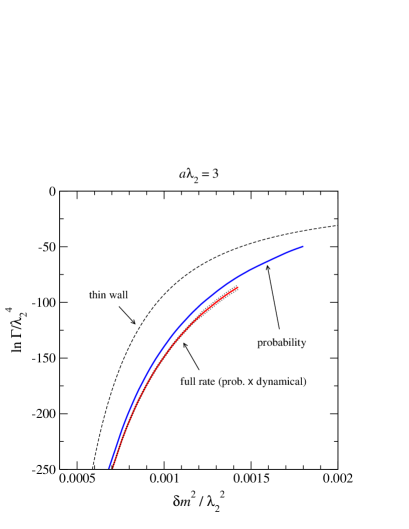
Figure 12: The rate of droplet nucleation $\Gamma/\lambda_{2}^{4}$ from $a\lambda_{2}=3$ lattices. The full rate curve contains all of the terms in Eq. (2.17), whereas the “probability” curve contains only the contribution $P_{C}^{\epsilon}/(V\lambda_{2}^{3})$. The thin wall curve is calculated using the surface tension and the latent heat measured from $a\lambda_{2}=3$ simulations.

Finally, let us pull together the ingredients discussed above and calculate the rate $\Gamma/\lambda_{2}^{4}$ with Eq. (2.17). First, note that since the dimension of $P_{C}^{\epsilon}$ is $[\phi^{2}_{{\rm av},{\rm lat}}]^{-1}=[a\phi^{2}_{{\rm av},{\rm cont.}}]^{-1}$, it does not have a good continuum limit by itself. In order to cancel the $a^{-1}$ factor, it is convenient to multiply $P_{C}^{\epsilon}/(V\lambda_{2}^{3})$ by $(a\lambda_{2})$ before extrapolation, and correspondingly divide $\langle|\Delta\phi^{2}_{\rm av}/\Delta t|\rangle\langle{\bf d}\rangle$ by it. (This is not an issue for $P(\phi^{2}_{{\rm av},C})/P(\phi^{2}_{{\rm av},{\rm SYM}})$ used in Sec. 5.1, since it is dimensionless.)

In Fig. 12 we show the nucleation rate $\Gamma/\lambda_{2}^{4}$ from $a\lambda_{2}=3$ lattices using $\gamma=0.0125$, where we have the most extensive set of data. In the “probability” curve we have set the product of the dynamical factors $1/(2a\lambda_{2})\langle|\Delta\phi^{2}_{\rm av}/\Delta t|\rangle\langle{\bf d}\rangle$ equal to $\lambda_{2}$ (this gives correct dimensions), and only the probability $P_{C}^{\epsilon}$ contributes to the rate. In the “full rate” curve we include the correct value of $\langle|\Delta\phi^{2}_{\rm av}/\Delta t|\rangle$ from Eq. (5.3), and ${\bf d}$ from Fig. 10, by substituting it with its average and making a conservative error estimate, ${\bf d}=0.08\pm 0.04$. In the final error estimate we also take into account the errors of $P_{C}^{\epsilon}$.

The inclusion of the dynamical factors reduce the rate by a factor of $\sim 10^{5}$. However, we emphasize that only the full rate is independent on the choice of observables. For example, if we simply switch from an intensive to an extensive order parameter, $P_{C}^{\epsilon}$, which is proportional to $1/\phi^{2}_{\rm av}$, would decrease by a factor $\propto 1/V$; this is compensated by a corresponding increase in $\langle|\Delta\phi^{2}_{\rm av}/\Delta t|\rangle$, so that the full rate remains invariant.

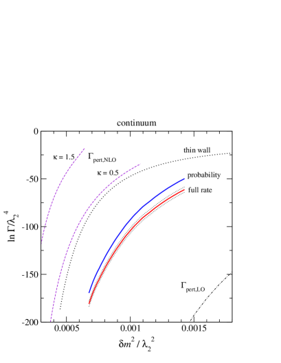
Figure 13: The nucleation rate as in Fig. 12, but extrapolated to the continuum limit. For comparison, we also show the rate calculated using the thin wall approximation and leading order and next-to-leading order perturbation theory. The curves labelled $\kappa=0.5$ and 1.5 show the scale sensitivity of the NLO calculation, see Sec. 6.2.

Next, let us consider the continuum limit extrapolation of the rate $\Gamma/\lambda_{a}^{4}$. The extrapolation of the probabilistic factor $P_{C}^{\epsilon}(a\lambda_{2})/(V\lambda_{2}^{3})$ alone proceeds as in Fig. 8; we fit an ansatz of form $c_{0}+c_{2}a^{3}$ independently at each $\delta m^{2}/\lambda_{2}^{2}$ to the lattice results from $a\lambda_{2}=2$, 2.5 and 3. The resulting curve is shown in Fig. 13. The remaining contribution to the rate is given by the dynamical factor $(a\lambda_{2})^{-1}\langle|\Delta\phi^{2}_{\rm av}/\Delta t|\rangle\langle{\bf d}\rangle$, which we assume to be constant as the lattice spacing is changed but the physical volume is kept constant. This quantity must have a continuum limit unless the dynamics posess some UV pathology. The simulation results from different lattice spacings do not show any lattice spacing dependence within statistical errors; however, errors are too large for a real continuum extrapolation.

The result of the extrapolation is shown in Fig. 13. The errors of the log of the rate are $\approx\pm 4$, including the errors coming from the extrapolation of $P_{C}^{\epsilon}$ and the estimated error from the extrapolation of ${\bf d}$. The error in $P_{C}^{\epsilon}$ dominates the uncertainty.

5.6 Droplet cross-sections

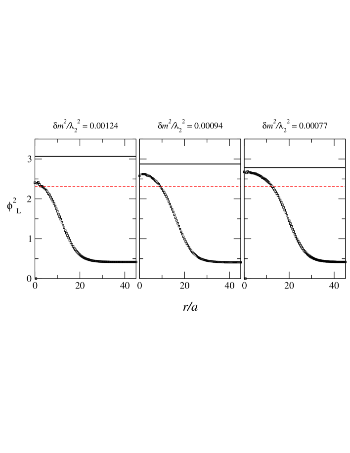
Figure 14: The droplet cross-sections at 3 different supecoolings from $a\lambda_{2}=3$, volume $80^{3}$ lattices. The expectation value $\langle\phi_{L}^{2}\rangle$ is shown in lattice units. The dotted line shows the broken phase $\langle\phi_{L}^{2}\rangle$ at the critical value of $m^{2}$, the solid lines at the supercooling $\delta m^{2}$. Only at the smallest supercooling does the core of the droplet approach the broken phase expectation value.

It is illuminating to take a closer look at the structure of the droplet configurations. Since the droplets are large objects in terms of correlation lengths, it is possible to perform suitable averaging over lattice configurations in order to measure the size and shape of critical bubbles at fixed supercooling. We do the averaging as follows:

• Generate a number of configurations with the constrained order parameter $|\phi^{2}_{\rm av}-\phi^{2}_{{\rm av},C}|<\epsilon$, where $\epsilon$ is a small number. These configurations contain a droplet of a fixed volume, as discussed in Sec. (2.1).

• Determine the center of the droplet. We do this by averaging the order parameter over $y,z$ coordinates, and taking the lowest non-trivial Fourer mode $A=\sum_{x}\phi^{2}(x)e^{i2\pi x/L}\,.$ The value $x_{0}=L/\pi\,\arctan(\mathrm{Im\,}A/\mathrm{Re\,}A)$ gives now the point around which the configuration is maximally symmetric. This is repeated for $y$ and $z$.

• Shift the origin to the center of the droplet, and determine the average order parameter as a function of the radius, $\phi^{2}(r)$. Averaging over the configurations we obtain the average droplet cross-section $\langle\phi^{2}(r)\rangle$.

We determined the droplet cross-sections for several different $m^{2}$ at $a\lambda_{2}=3$ lattices of size $80^{3}$, and in Fig. 14 we show the results for supercooling $\delta m^{2}/\lambda_{2}^{3}=0.00124$, 0.00094 and 0.00077. From Fig. 7 we see that these correspond to droplet free energies from 75 to 180. The droplet wall is very thick, and especially for smaller droplets there is no broken phase core to speak of. Thus, the thin wall approximation for the nucleation rate cannot be expected to work well. The expectation value $\langle\phi^{2}_{\rm av}\rangle$ is larger at the center of the droplet than the broken phase expectation value at $m_{c}^{2}$; this is naturally because the broken phase expectation value increases rapidly as $m^{2}$ is decreased. Only for the largest droplet (largest $m^{2}$) does the core approach the broken phase expectation value.

One can note that although the bulk of the droplets fits well on the lattice, at a smaller volume the exponentially decreasing tail of the fields outside the droplet wall would feel the lattice size. This decreases the free energy of the droplets, and it is no surprise that the $60^{3}$ lattice gives smaller droplet free energy at large droplets, see Fig. 7.

6 Comparison with other nucleation rate calculations

6.1 Thin wall approximation

The simplest semi-analytical estimate for the nucleation rate can be obtained using the thin wall approximation for the critical droplet free energy Eq. (2.5):

$$F_{TW}={\frac{16\pi\sigma^{3}}{3(\delta m^{2}\ell)^{2}}}\,,$$ (6.1)

where we use lattice determinations of the surface tension $\sigma$ and latent heat $\ell$. Thus, this method is not fully analytical; however, normally the determination of these values is an order of magnitude easier task than the full nucleation rate computation, and the thin wall approximation has often been used to include non-perturbative input in the nucleation rate calculations (see, for example, [33]).

The free energy is converted to a rate by multiplying it with suitable mass scale

$$\Gamma=m^{4}\exp-F_{TW}\,.$$ (6.2)

We use here the mass $m=0.05\lambda_{2}$, which is close to the symmetric phase perturbative mass; the precise value is not significant. The thin wall approximation assumes that the thickness of the droplet wall is negligible and that there are no contributions to the free energy due to the curvature of the walls. It becomes valid in the limit where the droplet radius is much larger than the thickness of the droplet wall; this condition is not usually well met in practice (see Sec. 5.6).

In Fig. 12 we show the thin wall result using the values of $\sigma$ and $\ell$ obtained from $a\lambda_{2}=3$ simulations. In the range of interest the thin wall rate is higher by $\sim e^{50}$. Large as the difference is, the thin-wall approximation is not as bad as one may first think: in many physical processes the system is cooled down at a very slow (constant) rate, and thus, the nucleation rate is changing with time: $d\Gamma/dt>0$. Since $\Gamma$ depends exponentially on $\delta m^{2}$, the transition occurs very rapidly when the nucleation rate reaches some critical value, typically $\Gamma_{c}\times l^{3}(t-t_{c})\sim 1$, where $l$ is some relevant length scale.

Let us take $\Gamma/\lambda_{2}^{4}=e^{-100}$ as our reference value. The lattice results from $\lambda_{2}=3$ give a supercooling value $\delta m^{2}/\lambda_{2}^{2}=0.00132(2)$, whereas the thin wall result is $0.00096(4)$, which is “only” $\sim 30$% smaller than the correct value. The errors of the thin wall results come from the errors of the determination of $\sigma$ and $\ell$.

In Fig. 13 we compare the lattice results to the thin wall ones at the continuum limit. Using again the reference value of $\Gamma_{c}/\lambda_{2}^{4}=e^{-100}$, the lattice result for the supercooling is $\delta m^{2}/\lambda_{2}^{2}=0.00094(3)$, and for the thin wall calculation $0.00063(7)$, again a 30% difference. Thus, the thin wall calculation gives a rather good order of magnitude estimate for the nucleation rate. This was also seen in the SU(2)-Higgs calculation in Ref. [19].

6.2 Perturbation theory

In the broken phase of the cubic anisotropy model (and with our choice of $\lambda_{1}/\lambda_{2}$) the field component which acquires a non-zero expectation value ($\phi_{1}$, say) is much lighter than the other field component ($\phi_{2}$). Due to this mass hierarchy, it turns out that we can calculate an effective potential (or action) for the $\phi_{1}$ field by perturbatively integrating over $\phi_{2}$. This effective potential can be used to calculate the leading contributions to the critical droplet free energy by finding the classical “bounce” solution to the equations of motion [34, 35, 36]. More concretely, assuming that the droplet is spherically symmetric and centered at $r=0$, we want to find a configuration $v(r)$ which is a saddle point of the action

$$S(m^{2})=4\pi\int_{0}^{\infty}dr\,r^{2}\,\left[{\frac{1}{2}}(\partial_{r}v)^{2}+V(m^{2};v)\right]\,.$$ (6.3)

Here $v$ is the expectation value of the scalar field. The boundary conditions are $v(\infty)=0$, $\partial_{r}v(0)=0$.

The dimensionless expansion parameter is proportional to the ratio of the two couplings $\lambda_{1}/\lambda_{2}$. This implies that the convergence becomes better the stronger the first order transition is (see Sec. 3). For our parameters the expansion parameter is $1/8\ll 1$, offering formally a good convergence parameter.

Without loss of generality we can choose the transition to happen in the direction of the $\phi_{1}$ field, and we shift the fields $(\phi_{1},\phi_{2})\rightarrow(v+\phi_{1},\phi_{2})$. The tree (mean field) level potential is

$$V_{0}(v)={\frac{1}{2}}m^{2}v^{2}+{\frac{1}{4!}}\lambda_{1}v^{4}$$ (6.4)

and the 1-loop potential is

$$V_{1}(v)=-{\frac{1}{12\pi}}(m_{1}^{3}+m_{2}^{3})\,,$$ (6.5)

where

$$m_{1}^{2}=m^{2}+{\frac{1}{2}}\lambda_{1}v^{2}\,,~{}~{}~{}~{}~{}~{}~{}~{}~{}m_{2}^{2}=m^{2}+{\frac{1}{2}}\lambda_{2}v^{2}\,.$$ (6.6)

In the broken phase, for $m^{2}$ close to the transition value, inspection of the potential gives the following power counting rules:

$$v^{2}\sim\lambda_{2}^{3}/\lambda_{1}^{2}~{}~{}~{}~{}\mbox{and}~{}~{}~{}~{}~{}m^{2}\sim\lambda_{2}^{3}/\lambda_{1}\,.$$ (6.7)

The leading contribution from the 1-loop term $m_{2}^{3}$ is of the same order as the tree level terms; it is just this third order term which makes the transition first order. On the other hand, the contribution from $m_{1}^{3}$ is suppressed by a factor $\propto(\lambda_{1}/\lambda_{2})^{3/2}$ in comparison to the leading order. This is actually subleading when compared with the leading 2-loop contributions; furthermore, at this order one also gets contributions from the resummation of the $\phi_{1}$ propagator, which render $m_{1}$ formally imaginary (easily seen by considering $V_{1}^{\prime\prime}(v)$, and equating this to $m_{1}^{2}$). It actually turns out that up to next-to-leading order in $\lambda_{1}/\lambda_{2}$ we do not have to consider the fluctuations of $\phi_{1}$ at all, justifying the use of the classical “bounce” solution at this order.

At the leading order we can also neglect $m^{2}$ in the expression for $m_{2}^{2}$, and write the potential as

$$V_{\rm LO}(v)=V_{0}(v)-{\frac{1}{24\sqrt{2}\pi}}\lambda_{2}^{3/2}v^{3}\,.$$ (6.8)

This potential gives a very strong first order transition, much stronger than the lattice calculations indicate, as can be seen by comparing the broken phase values $v^{2}$ and the surface tension $\sigma$ in Table 2. We calculate the perturbative surface tension from the integral

$$\sigma=\int_{v_{\rm symm.}}^{v_{\rm broken}}dv\sqrt{2V(v)}\,.$$ (6.9)

The droplet free energy (at some value of supercooling) can be solved from Eq. (6.3) numerically using the well-known undershoot/overshoot method [29]. (It can be solved analytically in some limiting cases, see, for example, [34].) As in the thin wall droplet case, we convert the droplet free energy to the nucleation rate using $\Gamma=m^{4}\exp(-F)$, where we use the mass scale $m=0.05\lambda_{2}$ (the result is insensitive to the precise value of $m$). Solving for the value of supercooling which gives the reference rate $\Gamma/\lambda_{2}^{4}=\exp-100$, we obtain the supercooling $\delta m^{2}=0.00234\lambda_{2}^{2}$, which is more than 100% larger than the result from the lattice simulations, Fig. 13 and Table 2.

The next-to-leading order corrections to the potential are suppressed relative to the leading terms by $\lambda_{1}/\lambda_{2}$. They arise from $m_{2}^{3}$ in Eq. (6.5), and from the leading two-loop contribution:

$$V_{2}(v)=V_{0}(v)-{\frac{1}{12\pi}}m_{2}^{3}-{\frac{v^{2}\lambda_{2}^{2}}{4(4\pi)^{2}}}\left[{\frac{1}{2}}\log{\frac{\mu^{2}}{2\lambda_{2}v^{2}}}+{\frac{1}{2}}\right]$$ (6.10)

The last term above is the two-loop contribution; it arises from the logarithmically divergent “sunset” diagram with two $\phi_{2}$ -propagators and one $\phi_{1}$-propagator, see Fig. 15. At this order we can neglect the masses from the propagators in the 2-loop diagram, and also the other 2-loop contributions (sunsets and figure-8 diagrams), which are suppressed by $(\lambda_{1}/\lambda_{2})^{3/2}$ or more.

Figure 15: Left: 2-loop “sunset” diagram used in the effective potential calculation. Right: the diagram used in the calculation of the wave function correction. The dotted lines are the “heavy” $\phi_{2}$ -propagators, and the solid lines correspond to the “light” $\phi_{1}$ propagators. The coupling constant at the vertices is $\lambda_{2}v$.

$v_{\rm broken}^{2}/\lambda_{2}$ $\sigma/\lambda_{2}^{2}$ $\delta m^{2}/\lambda_{2}^{2}$ $V_{\rm LO}$ 0.81 0.0124 0.0023 $V_{\rm NLO}$ $\kappa=0.5$ 0.44 0.0034 0.00058 $\kappa=1.5$ 0.40 0.0027 0.00033 lattice 0.49(1) 0.0050(2) 0.00094(3) thin wall - - 0.00063(7)

Table 2: Comparison of the perturbative, lattice and thin wall results. The supercooling has been evaluated at the point where the rate $\Gamma/\lambda_{2}^{4}=\exp(-100)$.

In Eq. (6.10) $\mu$ is the scale factor arising from dimensional regularization in $d=3-2\epsilon$ dimensions. As usual, a logarithmic divergence has been absorbed in a mass counterterm, which defines the scale dependent running mass

$$m_{R}^{2}(\mu)={\frac{\lambda_{2}^{2}}{2(4\pi)^{2}}}\log{\frac{\mu}{\Lambda}}\,.$$ (6.11)

We substitute $m^{2}$ with $m_{R}^{2}$ everywhere where it appears in the potential.

The dependence of $V(v)$ on the scale $\mu$ is formally of higher order than $\lambda_{1}/\lambda_{2}$; thus, we are free to choose $\mu$ so that the effect of the large logarithms in the potential are minimized. A common prescription is to fix $\mu$ so that the logarithm vanishes in the broken phase. Naturally, this does not suppress the logarithms in the symmetric phase at all. A better overall cancellation of the logs is achieved by using a $v$-dependent scale $\mu=2\kappa\sqrt{\lambda_{2}v^{2}/2}$, where $\kappa$ is a constant of order unity. However, this simple prescription is not complete, as discussed in Sec. 5 of Ref. [37]. Simplifying the renormalization arguments in the above reference a bit, this follows from the fact that the value of the effective potential is not a physical quantity, only the differences $V(v_{1})-V(v_{2})$ are, and the absolute value of the potential can have unphysical $\mu$-dependence. (Indeed, in dimensional regularization the value of the potential also at $v=0$ depends on the scale $\mu$.) Thus, if we change the renormalization point $\mu$ as we change $v$, the “normalization” of the potential changes, and it is not possible to directly compare $V(v_{1},\mu(v_{1}))$ and $V(v_{2},\mu(v_{2}))$ if $v_{1}$ and $v_{2}$ are far away from each other.

The most straightforward solution to this problem is to consider the slope of the potential $dV(v)/dv$ instead of the potential itself. With this quantity we can write a renormalization group improved expression for the next-to-leading order effective potential [37]:

$$V_{\rm NLO}(v^{\prime})=\int_{0}^{v^{\prime}}dv\left.{\frac{dV_{2}(v,\mu)}{dv}}\right|_{\displaystyle\mu=2\kappa\sqrt{\lambda_{2}v^{2}/2}}\,.$$ (6.12)

The derivative in the above expression is to be evaluated at fixed $\mu$, and only after taking the derivative $\mu$ is set to its optimized value.

In Table 2 we show $v^{2}_{\rm broken}$ and $\sigma$, calculated from potential (6.12), using values $\kappa=0.5$ and 1.5. The transition is weaker than the results from the lattice simulations; the broken phase expectation value of $v^{2}_{\rm broken}$ is 10-20% smaller, but the surface tension is around 40% smaller. Likewise, the supercooling $\delta m^{2}$ at rate $\Gamma=\lambda_{2}^{4}\exp(-100)$ is around 50% smaller than the lattice results. This discrepancy is of similar magnitude to the difference between perturbative and 2-loop results in the nucleation rate in SU(2)-Higgs theory [19]; however, in contrast to the cubic anisotropy model, the supercooling at a fixed value of the rate was seen to be larger in the perturbative analysis than on the lattice.

The scale dependence of the NLO nucleation rate is quite large in Table 2: the value of the supercooling increases by 75% when $\kappa$ is decreased from 1.5 to 0.5. This suggests that higher orders would affect the results significantly — this is, of course, already indicated by the fact that the NLO results do not agree well with the leading order results, or with the lattice. The large scale dependence is not a feature of the procedure to set $\mu$ used in Eq. (6.12): we can, for example, use the 2-loop potential (6.10) and just fix the scale $\mu$ so that the 2-loop contribution vanishes in the broken phase. If we vary $\mu$ by a factor of $\sim 50$%, the strength of the transition changes about as much as when we vary $\kappa$ in Eq. (6.12). Moreover, this method tends to give a somewhat weaker transition than Eq. (6.12).

In principle, finding the extremal critical droplet solution of the bounce action Eq. (6.3) with the NLO potential (6.12) does not give all of the $\mathcal{O}(\lambda_{1}/\lambda_{2})$ contributions. At this order one should take into account also the wave function correction  to the kinetic energy in the bounce action by modifying the second derivative term:

$$(\nabla v)^{2}\rightarrow(1+Z_{\phi})(\nabla v)^{2}\,.$$ (6.13)

The leading contribution to $Z_{\phi}$ can be calculated by evaluating the diagram on the right in Fig. 15 and expanding the result to second order in the external momentum (see, for example, Ref. [38]). This calculation is justified because $v$ (or $\phi_{1}$) varies on length scales $\sim m_{1}^{-1}$, which is much longer than the inverse mass of $\phi_{2}$, $m_{2}^{-1}$. The result of the calculation is

$$Z_{\phi}=-{\frac{\lambda_{2}^{2}v^{2}}{192\pi m_{2}^{3}}}\,,$$ (6.14)

which is indeed $\propto\lambda_{1}/\lambda_{2}$ according to the power counting rules, Eq. (6.7). However, the inclusion of the wave function correction modifies the results by less than 1%, which is a negligible effect considering the accuracy of the NLO calculation. This is in contrast to the SU(2) gauge + Higgs theory, where the wave function normalization was seen to improve the results dramatically. The reason for the smaller effect in this case is the very small numerical multiplicative factor in Eq. (6.14).

We can conclude that the NLO perturbative analysis at $\lambda_{1}/\lambda_{2}=1/8$ describes the phase transition qualitatively correctly, but the physical quantities can be a factor of 2–3 off the correct ones. Naturally, for $\lambda_{1}/\lambda_{2}$ closer to unity the NLO analysis would be even less accurate. The overall accuracy is comparable to the perturbative treatment of the SU(2) gauge + Higgs theory [19]. Trying to improve the perturbative treatment would require the calculation of contributions proportional to $(\lambda_{1}/\lambda_{2})^{3/2}$. At this order the light $\phi_{1}$ loops start to contribute, and, as mentioned above, $\phi_{1}$ propagators require resummation, which makes $m_{1}$ (and the 1-loop contribution in (6.5)) formally imaginary in the region where the second derivative of the effective potential is negative. Thus, it is not consistent to solve the effective potential in a constant background field as above; the correct treatment would require the calculation of the fluctuation determinant around a classical droplet solution. The simultaneous consistent (as a power series of $\lambda_{1}/\lambda_{2}$, say) evaluation of the fluctuation determinant and the effective potential is a very non-trivial problem, and we do not attempt it here.

6.3 Comparison with the coarse-grained effective action approach

The nucleation rate in the cubic anisotropy model was studied by Strumia and Tetradis using a coarse-graining approach [14]. First one calculates a coarse-grained effective action, valid for momentum scales smaller than a chosen scale $k$, where $k\mathop{\raise 1.29167pt\hbox{$<$\kern-7.5pt\raise-4.73611pt\hbox{$\sim$}}}m$, some physically relevant mass scale (for example, the mass of the light $\phi_{1}$ field in the broken phase, if the transition happens along the direction of $\phi_{1}$). Formally, the effective action is found by integrating out momenta $p>k$. In the second step, the nucleation rate is calculated using the effective action and Langer’s method: one finds the classical bounce solution (as in Sec. 6.2) with action $S_{k}$, around which the fluctuation determinant $A_{k}$ can be evaluated. The scale $k$ acts automatically as the ultraviolet regulator for the fluctuation determinant. The full rate is then estimated to be

$$\Gamma=A_{k}e^{-S_{k}}\,.$$ (6.15)

Since the physics does not care about the artificial scale $k$, the final result should be independent of $k$ if both halves of the calculation are under control.

The authors of Ref. [14] find the effective action using the renormalization group flow method of Wetterich [42]: they start from the bare action, Eq. (3.2), defined at some ultraviolet scale $k_{0}\gg k$, and use the flow equations to evolve the action down to scale $k$. During the evolution the action develops so that the resulting effective action has a first order transition already at “tree level”. It still contains both of the original fields. The evolution generates very complicated (non-local) effective actions, and in practical calculations the actions have to be truncated to a simple ansatz. For details, see Ref. [14] and references therein.

In Ref. [14] the nucleation rate is calculated at coupling constant ratios $\lambda_{1}/\lambda_{2}=0.3$ and $0.15$ (in their notation, $\lambda_{k_{0}}/g_{k_{0}}=0.1$ and 0.05, defined at the ultraviolet scale $k_{0}$.). The latter is close enough of the value we use here $\lambda_{1}/\lambda_{2}=1/8$ to make qualitative comparison possible. The results show a very strong dependence on the coarse graining scale $k$: for a fixed supercooling, the nucleation rate varies from $\ln\Gamma/m_{1}^{4}\approx-250$ to $-130$, when $k/m_{1}$ is changed from 0.6 to 0.9. Here $m_{1}$ is the mass of the light $\phi_{1}$ field in the broken phase. This implies that accuracy is lost during the calculation. Furthermore, the leading contribution to the rate does not come from $\exp(-S_{k})$, but from the fluctuation determinant $A_{k}$. This is partly caused by the fact that the mass of the $\phi_{2}$ field in the broken phase is much heavier than the coarse graining scale $k$, and gives a large contribution to the determinant. Indeed, one can argue that a coarse grained effective action where the heavy field is completely integrated out, as was done in Sec. 6.2, may offer a better starting point for the Langer method.

We should emphasize that the approach just described makes two separate approximations. The first is the truncation of the infrared effective action, made in the the renormalization group flow part of the calculation as the coarse graining scale is run down to $k$. This approximation means that some ultraviolet physics is lost or incorrectly incorporated in the coarse grained effective theory. The second approximation is in the calculation of the nucleation rate within the coarse grained theory itself; computing Gaussian fluctuations about a classical saddle point corresponds to carrying perturbation theory to one loop, neglecting interactions between infrared fluctuations. This is clearly not warranted if the infrared behavior is strongly coupled, for instance.

Since the dominant contribution does not come from the saddle point but from the fluctuation determinant, Langer’s method as a saddle point expansion fails in this calculation. However, our lattice simulations clearly indicate that a well-defined saddle point exists in the phase space. While the simulations make no distinction between the classical solution and the fluctuation determinant (everything is contained in the droplet free energy), the configurations at the saddle point consist of well-defined critical droplets. Thus, the physical picture given by Langer’s theory is valid; the problem in (semi)analytical calculations is to find the correct effective description.

7 Conclusion

In this paper we have used a novel technique for studying the critical droplet nucleation rate in first order phase transitions using non-perturbative lattice simulations. The method is readily applicable to exponentially small nucleation rates, which are often of relevance in physically interesting transitions. The technique consists of two separate stages: (1) the Monte Carlo evaluation of the nucleation barrier, using multicanonical methods, and (2) the correct treatment of the microscopic dynamics of the nucleation process with real time simulations. The first stage can be considered as a generalization of Langer’s theory of nucleation [4]: we have substituted the approximate saddle point expansion with a nonperturbative Monte Carlo calculation. The second step goes partly beyond Langer’s formalism. This method is readily applicable to any theory which is amenable to the lattice treatment in the first place, and, within the context of the lattice, the technique is exact up to exponentially small and in practice negligible corrections. This method has also been applied to the nucleation rate in SU(2)-Higgs theory [19]. Due to the multicanonical methods used, the statistical errors in the final answer tend to be automatically small — usually much smaller than any uncertainty in analytical approaches.

In this work we have applied the method to the phase transition in the cubic anisotropy model, which is a formally simple field theory with two scalar fields and a radiatively induced first order phase transition, the strength of which can be adjusted continuously. Because of the formal simplicity the theory is well suited for both analytical and numerical analyses. Since the transition is radiatively induced, Langer’s theory has to be applied with great care in analytical calculations.

We compare the nucleation rate obtained from the lattice simulation to customary analytical or semianalytical approaches. We find that the straightforward application of perturbation theory up to next-to-leading order in the relevant expansion parameter is not accurate: for a fixed value of the nucleation rate, the corresponding supercooling is roughly a factor 2 off the correct value, even though the scalar field expectation value is correct to within 15%. To go beyond the next-to-leading order would require the evaluation of the fluctuation determinant, and we did not attempt it in this work. On the other hand, a thin wall estimate, using non-perturbative input, is off only by 30%. The nucleation rate for a fixed supercooling is off even more than these numbers. This behaviour is strikingly similar to that observed in SU(2)-Higgs theory. The nucleation rate in the cubic anisotropy model has also been studied in Ref. [14], using an approximate coarse grained effective potential as a starting point for Langer’s procedure. The results were seen to depend very strongly on the coarse graining scale, making quantitative comparison impossible.

The results show that, for a rough-and-ready estimate of the nucleation rate, the thin wall approximation is acceptable, provided that one uses non-perturbatively determined surface tension and latent heat as an input. These are much easier to determine on the lattice than the full nucleation rate. On the other hand, the purely perturbative analysis shows weak convergence. If high accuracy is required, one has to resort to numerical evaluation.

Acknowlegments

We thank Dietrich Bödeker and Mikko Laine for many useful discussions. K.R. acknowledges partial support from EU TMR grant FMRX-CT97-0122. This work was partially supported by the DOE under contract DE-FGO3-96-ER40956.

Appendix A Renormalization of the lattice theory

This appendix details the matching calculation which eliminates $O(a^{2})$ errors in the lattice theory. This is done by computing a set of correlation functions in the lattice and continuum theories, at one and two loops, and adjusting the lattice couplings so the results coincide. The required correlation functions are the two and four point functions at zero momentum, the leading momentum dependence of the two point function, an insertion of $\langle\phi^{2}\rangle$ on a zero momentum line, and the vacuum value of the $\langle\phi^{2}\rangle$ operator. It is necessary only to find the difference between lattice and continuum values, to perform the matching; this difference is IR finite for all graphs we need. Each loop order eliminates errors at one higher power of $a$ because graphs become more UV convergent by one power per loop order in this 3 dimensional theory. For a more thorough discussion of how the matching calculation works, see [44].

A.1 results

A one loop lattice-continuum matching (renormalization) calculation will determine the $O(a)$ contributions to the quantities $Z_{\phi}$, $\delta\lambda$, and $Z_{m}$, and will find the $O(1/a)$ contributions to $\delta m^{2}$ and $\delta\langle\phi^{2}\rangle$. The required graphs are shown in Fig. 16. Evaluating the graphs requires choosing a lattice Laplacian. We consider two choices; the unimproved Laplacian

$$\nabla^{2}_{\rm U}\phi(x)=-6\phi(x)+\sum_{i}(\phi(x+i)+\phi(x-i))\,,$$ (1.1)

and the improved Laplacian, which we actually use:

$$\nabla^{2}_{\rm I}\phi(x)=-\frac{15}{2}\phi(x)+\frac{4}{3}\sum_{i}\Big{(}\phi(x+i)+\phi(x-i)\Big{)}-\frac{1}{12}\sum_{i}\Big{(}\phi(x+2i)+\phi(x-2i)\Big{)}\,.$$ (1.2)

We write the Fourier transforms of these choices as

$$\tilde{k}^{2}_{\rm U} = \sum_{i}(2-2\cos(k_{i}))\,,$$ (1.3)

$$\tilde{k}^{2}_{\rm I} = \sum_{i}\left(\frac{5}{2}-\frac{8}{3}\cos(k_{i})+\frac{1}{6}\cos(2k_{i})\right)\,.$$ (1.4)

The evaluation of the one loop graphs requires two integrals:

$$\frac{\Sigma}{4\pi} \equiv \int_{BZ}\frac{d^{3}k}{(2\pi)^{3}}\frac{1}{\tilde{k}^{2}}\,,$$ (1.5)

$$\frac{\xi}{4\pi} \equiv \int_{BZ}\frac{d^{3}k}{(2\pi)^{3}}\frac{1}{(\tilde{k}^{2})^{2}}-\int_{\Re^{3}}\frac{d^{3}k}{(2\pi)^{3}}\frac{1}{k^{4}}\,.$$ (1.6)

Here we use the shorthand $BZ$ to mean $k$ lies within the Brillouin zone, meaning each $k_{i}\in[-\pi,\pi]$. The integrals which determine $\xi$ are each IR singular and some regulation is implied, for instance adding $m^{2}$ to both $k^{2}$ and $\tilde{k}^{2}$ and taking the limit as $m^{2}\rightarrow 0$. The numerical values of the integrals are

$$\Sigma_{\rm U} = 3.17591153562522\,,\qquad\>\Sigma_{\rm I}=2.75238391130752\,,$$

$$\xi_{\rm U} = 0.152859324966101\,,\qquad\xi_{\rm I}=-0.083647053040968\,.$$ (1.7)

Note that the sign of $\xi$ depends on whether we use an improved lattice Laplacian. This is possible because $\xi$ represents the difference of a graph between lattice and continuum theories. The lattice contribution is larger inside the Brillouin zone, but the continuum integral receives contributions from outside the zone as well; the sign depends on which effect is larger.

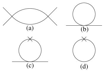
Figure 16: The one loop graphs needed for the renormalization. A cross represents a $\phi^{2}$ insertion.

At one loop the renormalizations are

$$\delta\lambda_{1,1l} = \left(\frac{3}{2}\lambda_{1}^{2}+\frac{3}{2}\lambda_{2}^{2}\right)\frac{\xi}{4\pi}\,,$$ (1.8)

$$\delta\lambda_{2,1l} = \left(\lambda_{1}\lambda_{2}+2\lambda_{2}^{2}\right)\frac{\xi}{4\pi}\,,$$ (1.9)

$$Z_{\phi,1l}-1 = 0\,,$$ (1.10)

$$Z_{m,1l}-1 = \left(\frac{1}{2}\lambda_{1}+\frac{1}{2}\lambda_{2}\right)\frac{\xi}{4\pi}\,,$$ (1.11)

$$\delta m^{2}_{1l} = -\left(\frac{1}{2}\lambda_{1}+\frac{1}{2}\lambda_{2}\right)\frac{\Sigma}{4\pi}\,,$$ (1.12)

$$\delta\langle\phi^{2}\rangle_{1l} = 2\frac{\Sigma}{4\pi}-2m^{2}\frac{\xi}{4\pi}\,.$$ (1.13)

Note that, if $\lambda_{1}=\lambda_{2},$ then $\delta\lambda_{1}=\delta\lambda_{2}$; and similarly if $\lambda_{1}=3\lambda_{2}$, then $\delta\lambda_{1}=3\delta\lambda_{2}$. Therefore the decoupling and $O(2)$ symmetric versions of the theory are preserved under renormalization.

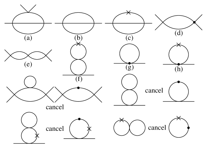
Figure 17: All required two loop graphs and one loop graphs with one loop counterterm insertions, shown as heavy dots on lines (mass counterterms) or at vertices (coupling counterterms). The last eight graphs cancel in pairs. Diagrams (a), (d), and (e) are not separately IR convergent; diagram (d) must be distributed between the other two to produce IR convergent integrals.

It makes no sense to carry the matching to two loops unless we use the improved lattice Laplacian, as $O(a^{2})$ errors would already appear at two loop level. The two loop results require several more graphs and the inclusions in one loop graphs of the one loop mass and coupling counterterms, see Fig. 17. Three more integrals are needed, and their evaluation is detailed in the appendix. The complete two loop renormalization is given by

$$\delta\lambda_{1}-\delta\lambda_{1,1l} = -\left(3\lambda_{1}^{3}+3\lambda_{1}\lambda_{2}^{2}+6\lambda_{2}^{3}\right)\frac{C_{1}}{16\pi^{2}}+\left(\frac{3}{4}\lambda_{1}^{3}+\frac{9}{4}\lambda_{1}\lambda_{2}^{2}\right)\left(\frac{\xi}{4\pi}\right)^{2},$$ (1.14)

$$\delta\lambda_{2}-\delta\lambda_{2,1l} = -\left(\lambda_{1}^{2}\lambda_{2}+6\lambda_{1}\lambda_{2}^{2}+5\lambda_{2}^{3}\right)\frac{C_{1}}{16\pi^{2}}+\left(\frac{3}{4}\lambda_{1}^{2}\lambda_{2}+\frac{9}{4}\lambda_{2}^{3}\right)\left(\frac{\xi}{4\pi}\right)^{2},$$ (1.15)

$$Z_{\phi}-1 = \left(\frac{1}{6}\lambda_{1}^{2}+\frac{1}{2}\lambda_{2}^{2}\right)\frac{C_{2}}{16\pi^{2}}\,,$$ (1.16)

$$Z_{m}-Z_{m,1l} = \frac{1}{4}(\lambda_{1}+\lambda_{2})^{2}\left(\frac{\xi}{4\pi}\right)^{2}-\left(\frac{1}{2}\lambda_{1}^{2}+\frac{3}{2}\lambda_{2}^{2}\right)\left(\frac{C_{1}}{16\pi^{2}}\right)\,,$$ (1.17)

$$\delta m^{2}-\delta m^{2}_{1l} = \left(\frac{1}{6}\lambda_{1}^{2}+\frac{1}{2}\lambda_{2}^{2}\right)\frac{1}{16\pi^{2}}\left(\ln\frac{6}{a\mu}+C_{3}\right)$$ (1.18)

$$-\left(\frac{\delta\lambda_{1}}{2}+\frac{\delta\lambda_{2}}{2}\right)\frac{\Sigma}{4\pi}+(1-Z_{m,1l})\delta m^{2}_{1l}$$

$$\delta\langle\phi^{2}\rangle-\delta\langle\phi^{2}\rangle_{1l} = \left(\lambda_{1}+\lambda_{2}\right)\frac{\xi\Sigma}{16\pi^{2}}\,.$$ (1.19)

Three new numerical constants appear here; their numerical values are $C_{1}=.0550612,$ $C_{2}=.0334416,$ and $C_{3}=-.86147916$. $\delta m^{2}$ and $\delta\langle\phi^{2}\rangle$ can be defined when using Eq. (1.1), in which case $C_{3,{\rm U}}=.08848010$; but the other improvements do not make sense and should not be applied if that Laplacian is used. We can again check that the form of $\delta\lambda_{1}$ and $\delta\lambda_{2}$ is consistent at the two special values $\lambda_{1}=\lambda_{2}$ and $\lambda_{1}=3\lambda_{2}$.

It is possible in principle to extend the improvement scheme to $O(a^{3})$, by making a three loop calculation. However, at this order it is necessary to include mixing of different dimensions of operator insertions and to include counterterms for radiatively induced high dimension operators in the Lagrangian. The calculation of the graphs also becomes significantly more challenging. The improvement presented here is sufficient for our purposes; the leading lattice spacing errors in measurables related to the strength of the phase transition now first appear at $O(a^{3})$.

A.2 Two loop graphs

Here we detail the calculation of $C_{1}$, $C_{2}$, and $C_{3}$.

We begin with the two loop vertex correction, Figure 17 graph (a). The required integral, including the appropriate amount of the one loop counterterm graph (d), is

$$\frac{C_{1}}{16\pi^{2}}=\int_{k,BZ}\frac{1}{(\tilde{k}^{2})^{2}}\left\{\int_{l,BZ}\frac{1}{\tilde{l}^{2}\widetilde{(k+l)}^{2}}-\frac{\xi}{4\pi}\right\}-\int_{k,\Re^{3}}\frac{1}{k^{4}}\int_{l,\Re^{3}}\frac{1}{l^{2}(k+l)^{2}}\,.$$ (1.20)

Here we use the shorthand in which the integration limit also lists which variable is being integrated over; so $\int_{k,BZ}$ means $\int_{[-\pi,\pi]^{3}}(d^{3}k/(2\pi)^{3})$. The first step is to evaluate the inner continuum integral, which can be done by standard Feynman parameter methods;

$$\int_{l,\Re^{3}}\frac{1}{l^{2}(k+l)^{2}}=\int_{0}^{1}d\alpha\frac{1}{2\pi^{2}}\int_{0}^{\infty}\frac{l^{2}dl}{(l^{2}+\alpha(1-\alpha)k^{2})^{2}}=\frac{1}{8k}\,.$$ (1.21)

Then we re-arrange the original integral into three parts,

$$\int_{k,BZ}\frac{1}{(\tilde{k}^{2})^{2}}\left\{\int_{l,BZ}\frac{1}{\tilde{l}^{2}\widetilde{(k+l)}^{2}}-\frac{1}{8k}-\frac{\xi}{4\pi}\right\}+\int_{k,BZ}\frac{1}{8k}\left(\frac{1}{(\tilde{k}^{2})^{2}}-\frac{1}{k^{4}}\right)-\int_{k,\Re^{3}-BZ}\frac{1}{8k^{5}}\,.$$ (1.22)

The first integral is IR well behaved because the two counterterms cancel the $l$ integral up to a $k^{2}$ correction, which in the small $k$ limit is $.0125438k^{2}/4\pi$. The integrals can be performed by quadratures using adaptive mesh refinement techniques and Richardson extrapolation. The first integral gives $.0360003/16\pi^{2}$ and the second gives $.054568958/16\pi^{2}$. The last integral, over $\Re^{3}-BZ$, can be re-arranged into

$$-\frac{3}{16\pi^{5}}\int_{0}^{1}dx\int_{0}^{1}dy\frac{1}{(1+x^{2}+y^{2})^{5/2}}=\frac{-.035507296027\ldots}{16\pi^{2}}\,.$$ (1.23)

These sum to give $C_{1}=.0550612$.

Besides this graph there is graph (e), which gives

$$\left(\int_{k,BZ}\frac{1}{(\tilde{k}^{2})^{2}}\right)^{2}-\left(\int_{k,\Re^{3}}\frac{1}{k^{4}}\right)^{2}\,,$$ (1.24)

which is not IR convergent; however, including -2 times the counterterm diagram (d),

$$-2\left(\int_{k,BZ}\frac{1}{(\tilde{k}^{2})^{2}}\right)\left(\int_{k,BZ}\frac{1}{(\tilde{k}^{2})^{2}}-\int_{k,\Re^{3}}\frac{1}{k^{4}}\right)\,,$$ (1.25)

gives $-(\xi/4\pi)^{2}$; no new integrals are required. It is a nontrivial check on the calculation that the sum of the coefficients arising from diagrams (a) and (e) precisely absorb diagram (d).

The next integral is the $O(p^{2})$ contribution from the setting sun diagram (b),

$$\frac{C_{2}}{16\pi^{2}} = \lim_{p\rightarrow 0}\frac{1}{p^{2}}\Bigg{\{}\int_{k,BZ}\left[\left(\frac{1}{\widetilde{(k+p)}^{2}}-\frac{1}{\tilde{k}^{2}}\right)\left(\int_{l,BZ}\frac{1}{\tilde{l}^{2}\widetilde{(k+l)}^{2}}\right)\right]$$ (1.26)

$$\qquad\qquad-\int_{k,\Re^{3}}\left[\left(\frac{1}{(k+p)^{2}}-\frac{1}{k^{2}}\right)\left(\int_{l,\Re^{3}}\frac{1}{l^{2}(k+l)^{2}}\right)\right]\Bigg{\}}\,.$$

The first trick is to note that

$$\int_{k,BZ}\left(\frac{1}{\widetilde{(k+p)}^{2}}-\frac{1}{\tilde{k}^{2}}\right)=0$$ (1.27)

just by shifting the integration variable for the first term; so we may add $-\xi/4\pi$ to the term in the second parenthesis of the first line of Eq. (1.26). This prevents IR divergences in what follows, so we are free to expand $1/\widetilde{(k+p)}^{2}$ to second order in $p$; after averaging over directions for $p$, we find

$$\frac{1}{\widetilde{(k+p)}^{2}}-\frac{1}{\tilde{k}^{2}}=p^{2}\left[\frac{\frac{1}{3}\sum_{i}\left(\frac{8\sin k_{i}-\sin 2k_{i}}{3}\right)^{2}}{(\tilde{k}^{2})^{3}}-\frac{\frac{1}{3}\sum_{i}\left(\frac{4\cos k_{i}-\cos 2k_{i}}{3}\right)}{(\tilde{k}^{2})^{2}}\right]\equiv p^{2}{\cal M}(k)\,.$$ (1.28)

The equivalent expression in the continuum case is $(p^{2}/3)/k^{4}$. Re-arranging the terms a little, we can write

$$\frac{C_{2}}{16\pi^{2}} = -\frac{1}{24}\int_{k,\Re^{3}-BZ}\frac{1}{k^{5}}+\int_{k,BZ}\frac{1}{8k}\left({\cal M}(k)-\frac{(1/3)}{k^{4}}\right)$$ (1.29)

$$+\int_{k,BZ}{\cal M}(k)\left[\int_{l,BZ}\frac{1}{\tilde{l}^{2}\widetilde{(k+l)}^{2}}-\frac{1}{8k}-\frac{\xi}{4\pi}\right]\,.$$

The first integral is (1/3) of Eq. (1.23). The second gives $.0310757695/16\pi^{2}$ and the last gives $.0142016/16\pi^{2}$, so $C_{2}=.0334416$.

Next we must compute the $O(p^{0})$ part of the setting sun diagram. The continuum diagram is log IR and UV divergent, while the lattice diagram is only log IR divergent. It is convenient to IR regulate both by introducing a mass on one line. In this case the continuum integral can be performed in $\overline{\rm MS}$, leaving a lattice integral minus an analytically determined counterterm [37, 45]. Choosing to separate the renormalization dependence along with the same finite constant as in the previous literature [37, 45], the constant $C_{3}$ is given by

$$\frac{C_{3}}{16\pi^{2}}=\lim_{m\rightarrow 0}\left\{\int_{k,BZ}\frac{1}{\tilde{k}^{2}+m^{2}}\int_{l,BZ}\frac{1}{\tilde{l}^{2}\widetilde{(k+l)}^{2}}-\frac{1}{16\pi^{2}}\left[\frac{1}{2}+\ln\frac{6}{m}\right]\right\}\,.$$ (1.30)

The annoying feature of this expression is the logarithm. To remove it, we add and subtract $1/8k$ to the integral over $l$. The integral

$$\int_{k,BZ}\frac{1}{\tilde{k}^{2}+m^{2}}\left[\int_{l,BZ}\frac{1}{\tilde{l}^{2}\widetilde{(k+l)}^{2}}-\frac{1}{8k}\right]$$ (1.31)

is IR convergent and the $m\rightarrow 0$ limit may be taken immediately. It evaluates to $-.06858432/16\pi^{2}$, unless we use the unimproved lattice Laplacian, in which case it is $.60953343/16\pi^{2}$. We re-arrange the remaining terms to be

$$\int_{k,BZ}\left(\frac{1}{\tilde{k}^{2}+m^{2}}-\frac{1}{k^{2}+m^{2}}\right)\frac{1}{8k}+\int_{k,BZ}\frac{1}{8k(k^{2}+m^{2})}-\frac{1}{16\pi^{2}}\left[\frac{1}{2}+\frac{6}{m}\right]\,.$$ (1.32)

Again, for the first integral the $m\rightarrow 0$ limit may be taken immediately, and the numerical value is $.161799607/16\pi^{2}$, or $.43364112015/16\pi^{2}$ if we use the unimproved Laplacian. For the last integral, we cut the integration region into the ball of radius $\pi$ and the region within the Brillouin zone but outside the ball:

$$\int_{k,BZ}\frac{1}{8k(k^{2}+m^{2})}=\frac{1}{2\pi^{2}}\int_{0}^{\pi}\frac{k^{2}dk}{8k(k^{2}+m^{2})}+\int_{k,BZ}\frac{1}{8k(k^{2}+m^{2})}\Theta(|k|-\pi)\,.$$ (1.33)

The former may be promptly integrated to give $\ln(\pi/m)/16\pi^{2}$ plus terms power suppressed in $m$; when added to $(-1/16\pi^{2})(\ln(6/m)+1/2)$ this cancels the $\ln(m)$, leaving $(1/16\pi^{2})(\ln(\pi/6)-1/2)$. The final integral has had the small $k$ part of the integration range removed, so again the $m\rightarrow 0$ limit may be taken. It can then be reduced to

$$\frac{1}{16\pi^{2}}\int\frac{d\Omega}{4\pi}\ln(R({\rm cube})-R({\rm ball}))=\frac{1}{16\pi^{2}}\frac{12}{\pi}\int_{0}^{\pi/4}d\phi\int_{0}^{{\rm arctan}(\sec\phi)}\sin(\theta)d\theta\ln(\sec(\theta))$$ (1.34)

which numerically equals $.19233513195/16\pi^{2}$. Note that at no point have we had to deal numerically with an integral which is log divergent in $m$, or which still contains $m$ at all.

Combining terms gives $C_{3}=-.86147916$, unless we use the unimproved lattice Laplacian, in which case it is $C_{3}=.08848010$. In the notation of [37, 45], $C_{3}$ is called $\zeta$. Note that, unlike $C_{1}$ and $C_{2}$, $C_{3}$ is relatively large. Similarly, $\xi$ is small but $\Sigma$ is large. This means that the radiative $O(a)$ and $O(a^{2})$ corrections to quantities which do not renormalize in the continuum are all small, but the corrections to the mass are larger. The size of $C_{3}$ also depends on a somewhat arbitrary choice to make it accompany $\ln(6/a\mu)$.

References

- [1] V. A. Rubakov and M. E. Shaposhnikov, Usp. Fiz. Nauk166 (1996) 493, Phys. Usp. 39 (1996) 461, [hep-ph/9603208].
- [2] R. Becker and W. Döring, Annals Phys. 24 (1935) 719.
- [3] J.W. Cahn and J.E. Hilliard, J. Chem. Phys. 31 (1959) 688.
- [4] J. S. Langer, Annals Phys. 41 (1967) 108; ibid. 54 (1969) 258.
- [5] J.D. Gunton and M. Droz, Introduction to the Theory of Metastable and Unstable States, Springer-Verlag, Berlin (1983).
- [6] C. Callan and S. Coleman, Phys. Rev. D 16 (1977) 1762.
- [7] M. B. Voloshin, I. Y. Kobzarev and L. B. Okun, Sov. J. Nucl. Phys. 20 (1975) 644, Yad. Fiz. 20 (1974) 1229.
- [8] I. Affleck, Phys. Rev. Lett. 46 (1981) 388.
- [9] A. D. Linde, Nucl. Phys. B216 (1983) 421, Erratum-ibid. B223 (1983) 544.
- [10] G.D. Moore, K. Rummukainen and A. Tranberg, to be published in the proceedings of the conference Strong and Electroweak Matter 2000, ed. C. Korthals Altes, [hep-lat/0101018].
- [11] J. Rudnick, Phys. Rev. B11 (1975) 3397.
- [12] P. Arnold and L. G. Yaffe, Phys. Rev. D55 (1997) 7760 [hep-ph/9610447]; P. Arnold and Y. Zhang, Phys. Rev. D 55 (1997) 7776 [hep-ph/9610448].
- [13] P. Arnold, S. R. Sharpe, L. G. Yaffe and Y. Zhang, Phys. Rev. Lett. 78 (1997) 2062 [hep-ph/9611201].
- [14] A. Strumia and N. Tetradis, Nucl. Phys. B554 (1999) 697 [hep-ph/9811438]; JHEP9911 (1999) 023 [hep-ph/9904357].
- [15] D. Stauffer, A. Coniglio and D.W. Heermann, Phys. Rev. Lett. 49 (1982) 1299; K. Binder, Phys. Rev. A 25 (1982) 1699; M. Acharyya and D. Stauffer, [cond-mat/9801213]; P.A. Rikvold et al, in Computer Simulation Studies in Condensed Matter Physics XII, edited by D.P. Landau et al., Springer Proceedings in Physics Vol. 85 (Springer, Berlin, 2000).
- [16] H. Arkin, T. Çelik, B.A. Berg and H. Meyer-Ortmanns, Int. J. Mod. Phys. C 10 (1999) 1261.
- [17] S. Borsanyi, A. Patkos, J. Polonyi and Z. Szep, Phys. Rev. D 62 (2000) 085013 [hep-th/0004059].
- [18] M. A. Novotny, Int. J. Mod. Phys. C 10 (1999) 1483 [cond-mat/9909158].
- [19] G. D. Moore and K. Rummukainen, Phys. Rev. D 63 (2001) 045002 [hep-ph/0009132].
- [20] G. D. Moore, Phys. Lett. B439 (1998) 357 [hep-ph/9801204]; Phys. Rev. D59 (1999) 014503 [hep-ph/9805264].
- [21] B. A. Berg and T. Neuhaus, Phys. Lett. B267 (1991) 249; Phys. Rev. Lett. 68 (1992) 9 [hep-lat/9202004].
- [22] K. Binder, Phys. Rev. A 25 (1982) 1699.
- [23] S. Coleman and E. Weinberg, Phys. Rev. D7 (1973) 1888.
- [24] D. Bödeker, Nucl. Phys. B486 (1997) 500 [hep-th/9609170].
- [25] G. Aarts and J. Smit, Nucl. Phys. B511 (1998) 451 [hep-ph/9707342].
- [26] A. M. Horowitz, Phys. Lett. B156 (1985) 89
- [27] S. Ryang, T. Saito and K. Shigemoto, Prog. Theor. Phys. 73 (1985) 1295.
- [28] S. Jeon, Phys. Rev. D 52 (1995) 3591 [hep-ph/9409250].
- [29] W.H. Press, B.P. Flannery, S.A. Teukolsky and W.T. Vetterling, Numerical Recipes, second edition, Cambridge University Press, Cambridge 1992.
- [30] M. Laine and K. Rummukainen, Nucl. Phys. B535 (1998) 423 [hep-lat/9804019].
- [31] B. A. Berg, Nucl. Phys. Proc. Suppl. 63 (1998) 982 [hep-lat/9708003].
- [32] B. Bunk, Int. J. Mod. Phys. C 3 (1992) 889.
- [33] Y. Iwasaki, K. Kanaya, L. Kärkkäinen, K. Rummukainen and T. Yoshié, Phys. Rev. D 49 (1994) 3540 [hep-lat/9309003].
- [34] K. Enqvist, J. Ignatius, K. Kajantie and K. Rummukainen, Phys. Rev. D 45 (1992) 3415.
- [35] N. Turok, Phys. Rev. Lett. 68 (1992) 1803.
- [36] M. Dine, R. G. Leigh, P. Huet, A. Linde and D. Linde, Phys. Rev. D46 (1992) 550 [hep-ph/9203203].
- [37] K. Farakos, K. Kajantie, K. Rummukainen and M. Shaposhnikov, Nucl. Phys. B442 (1995) 317 [hep-lat/9412091].
- [38] D. Bödeker, W. Buchmuller, Z. Fodor and T. Helbig, Nucl. Phys. B423 (1994) 171 [hep-ph/9311346].
- [39] G. Münster and S. Rotsch, Eur. Phys. J. C12 (2000) 161 [cond-mat/9908246].
- [40] J. Baacke, Phys. Rev. D52 (1995) 6760 [hep-ph/9503350].
- [41] A. Parnachev and L. G. Yaffe, Phys. Rev. D 62 (2000) 105034 [hep-th/0005269].
- [42] C. Wetterich, Phys. Lett. B301 (1993) 90.
- [43] E. J. Weinberg, Phys. Rev. D 47 (1993) 4614 [hep-ph/9211314].
- [44] G. D. Moore, Nucl. Phys. B 493 (1997) 439 [hep-lat/9610013]; G. D. Moore, Nucl. Phys. B 523 (1998) 569 [hep-lat/9709053].
- [45] M. Laine and A. Rajantie, Nucl. Phys. B513 (1998) 471 [hep-lat/9705003].