Determination of $\mathbf{\Lambda_{\overline{MS}}}$ from quenched and $\mathbf{N_{f}=2}$ dynamical QCD

Abstract

The scale parameter $\Lambda_{\overline{MS}}$ is computed on the lattice in the quenched approximation and for $N_{f}=2$ flavors of light dynamical quarks. The dynamical calculation is done with non-perturbatively $O(a)$ improved Wilson fermions. In the continuum limit we obtain $\Lambda_{\overline{MS}}^{N_{f}=0}=243(1)(10)\,\mbox{MeV}$ and $\Lambda_{\overline{MS}}^{N_{f}=2}=217(16)(11)\,\mbox{MeV}$, respectively.

, , , ,  ,  , , , ,  ,

– QCDSF–UKQCD Collaboration –

1 Introduction

The $\Lambda$ parameter sets the scale in QCD. In the chiral limit it is the only parameter of the theory, and hence it is a quantity of fundamental interest. It is defined by the running of the strong coupling constant $\alpha_{s}$ [1] at high energies where non-perturbative effects are supposed to become small. Lattice gauge theory provides a means of determining $\alpha_{s}$ directly from low-energy quantities. In this letter we shall compute $\Lambda$ on the lattice in the quenched approximation as well as for $N_{f}=2$ species of degenerate dynamical quarks.

Previous lattice calculations have employed a variety of methods to compute the strong coupling constant, in quenched and unquenched simulations. For reviews see [2, 3]. The scale parameter $\Lambda$ has been extracted from the heavy-quark potential [4, 5, 6], the quark-gluon vertex [7], the three-gluon vertex [8, 9], from the spectrum of heavy quarkonia [10, 11, 12, 13, 14], and by means of finite-size-scaling methods [15].

We determine $\Lambda$ from the average plaquette and the force parameter $r_{0}$ [16]. Both quantities are widely computed in lattice simulations. In the quenched case we have many data points over a wide range of couplings at our disposal already, and in the dynamical case we expect to accumulate more points in the near future. At present $r_{0}$ is the best known lattice quantity, at least in full QCD. It can easily be replaced with more physical scale parameters like hadron masses or $f_{\pi}$ when the respective data become more accurate.

2 Method

The calculations are done with the standard gauge field action

$$S_{G}=\beta\sum_{x}\mbox{Re}\,\frac{1}{3}\mbox{Tr}U_{\Box}(x),$$ (1)

and, in the dynamical case, with non-perturbatively $O(a)$ improved Wilson fermions [17]

$$S_{F}=S^{(0)}_{F}-\frac{\rm i}{2}\kappa_{\rm sea}\,g\,c_{SW}aa^{4}\sum_{x}\bar{\psi}(x)\sigma_{\mu\nu}F_{\mu\nu}\psi(x),$$ (2)

where $S^{(0)}_{F}$ is the original Wilson action and $\beta=6/g^{2}$. If the improvement coefficient $c_{SW}$ is appropriately chosen, this action removes all $O(a)$ errors from on-shell quantities. A non-perturbative evaluation of this function leads to the parameterization [18]

$$c_{SW}=\frac{1-0.454g^{2}-0.175g^{4}-0.012g^{6}+0.045g^{8}}{1-0.720g^{2}}$$ (3)

for $N_{f}=2$ flavors, which is valid for $\beta\geq 5.2$.

The running of the coupling is described by the $\beta$ function defined by

$$\mu\frac{\partial g_{\mathcal{S}}(\mu)}{\partial\mu}=\beta^{\mathcal{S}}(g_{\mathcal{S}}(\mu)),$$ (4)

where $\mathcal{S}$ is any mass independent renormalization scheme. The perturbative expansion of the $\beta$ function reads

$$\beta^{\mathcal{S}}(g_{\mathcal{S}})=-g_{\mathcal{S}}^{3}\,\big{(}b_{0}+b_{1}g_{\mathcal{S}}^{2}+b_{2}^{\mathcal{S}}g_{\mathcal{S}}^{4}+b_{3}^{\mathcal{S}}g_{\mathcal{S}}^{6}+\cdots\;\big{)}.$$ (5)

The first two coefficients are universal,

$$\begin{split}b_{0}&=\frac{1}{(4\pi)^{2}}\big{(}11-\frac{2}{3}N_{f}\big{)},\\ b_{1}&=\frac{1}{(4\pi)^{4}}\big{(}102-\frac{38}{3}N_{f}\big{)},\end{split}$$ (6)

while the others are scheme dependent. The renormalization group equation (4) can be exactly solved:

$$\frac{\mu}{\Lambda_{\mathcal{S}}}=\big{(}b_{0}g_{\mathcal{S}}^{2}\big{)}^{\frac{b_{1}}{2b_{0}^{2}}}\,\exp\Big{(}\frac{1}{2b_{0}g_{\mathcal{S}}^{2}}+\int_{0}^{g_{\mathcal{S}}}{\rm d}\xi\;\big{(}\frac{1}{\beta^{\mathcal{S}}(\xi)}+\frac{1}{b_{0}\xi^{3}}-\frac{b_{1}}{b_{0}^{2}\xi}\big{)}\Big{)},$$ (7)

where the scale parameter $\Lambda$ appears as the integration constant. In the $\overline{MS}$ scheme the $\beta$ function is known to four loops [19]:

$$\begin{split}b_{2}^{\overline{MS}}&=\frac{1}{(4\pi)^{6}}\big{(}\frac{2857}{2}-N_{f}\frac{5033}{18}+N_{f}^{2}\frac{325}{54}\big{)},\\[10.00002pt] b_{3}^{\overline{MS}}&=\frac{1}{(4\pi)^{8}}\Big{(}\frac{149753}{6}+3564\,\zeta_{3}-N_{f}\big{(}\frac{1078361}{162}+\frac{6508}{27}\,\zeta_{3}\big{)}\\ &\hskip 51.21504pt+N_{f}^{2}\big{(}\frac{50065}{162}+\frac{6472}{81}\,\zeta_{3}\big{)}+N_{f}^{3}\frac{1093}{729}\Big{)},\end{split}$$ (8)

where $\zeta_{3}=1.20206\cdots$ is Riemann’s zeta function.

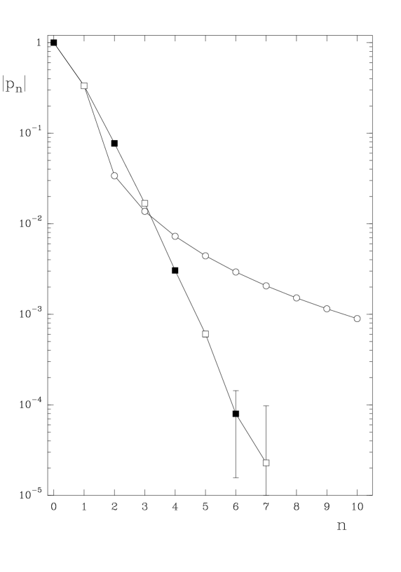
Figure 1: The expansion coefficients for the quenched plaquette, $1-P=\sum_{n=1}^{\infty}p_{n}x^{n}$, for $x=g^{2}$ ($\circ$) and $x=g_{\Box}^{2}$ ($\square$ and $\blacksquare$), respectively. Open (solid) symbols refer to positive (negative) numbers. The bare expansion coefficients ($\circ$) are taken from [21]. Note that the boosted coefficients are not only much smaller and rapidly decreasing, but also alternating in sign.

In this paper we are concerned with three different schemes. In the continuum we use the $\overline{MS}$ scheme. On the lattice we consider the bare coupling $g(a)$ and the boosted coupling $g_{\Box}(a)$. The latter is given by

$$g^{2}_{\Box}(a)=\frac{g^{2}(a)}{P},$$ (9)

where $P=(1/3)\>\langle\mbox{Tr}U_{\Box}\rangle\equiv u_{0}^{4}$ is the average plaquette value. The widespread opinion is that the perturbative expansion in $g_{\Box}$ converges more rapidly than the expansion in the bare coupling [20]. Indeed, a comparison between the expansion coefficients in the two cases for the quenched plaquette shown in Fig. 1 supports this belief, as even for low orders the new series has oscillating coefficients. The conversion from the bare coupling to the $\overline{MS}$ scheme has the form

$$\frac{1}{g_{\overline{MS}}^{2}(\mu)}=\frac{1}{g^{2}(a)}+2b_{0}\ln a\mu-t_{1}+(2b_{1}\ln a\mu-t_{2})\,g^{2}(a)+O(g^{4}\ln^{2}a\mu).$$ (10)

Writing

$$\frac{1}{g_{\Box}^{2}}=\frac{1}{g^{2}}-p_{1}-p_{2}g^{2}-p_{3}g^{4}-\cdots,$$ (11)

we obtain the relation between the boosted coupling and the $\overline{MS}$ coupling

$$\begin{split}\frac{1}{g_{\overline{MS}}^{2}(\mu)}&=\frac{1}{g_{\Box}^{2}(a)}+2b_{0}\ln a\mu-t_{1}+p_{1}\\ &+(2b_{1}\ln a\mu-t_{2}+p_{2})\,g^{2}_{\Box}(a)+O(g^{4}\ln^{2}a\mu).\end{split}$$ (12)

By differentiating eq. (12) we can find the $\beta$ function coefficient, $b_{2}^{\Box}$, for the boosted coupling

$$b_{2}^{\Box}=b_{2}^{\overline{MS}}+b_{0}(p_{2}-t_{2})-b_{1}(p_{1}-t_{1}).$$ (13)

The one-loop coefficients $p_{1}$ and $t_{1}$ are given by

$$p_{1} =\frac{1}{3},$$ (14)

$$t_{1} =0.4682013-N_{f}\big{(}0.0066960-0.0050467\,c_{SW}+0.0298435\,c_{SW}^{2}$$

$$\hskip 11.38092pt+am(-0.0272837+0.0223503\,c_{SW}-0.0070667\,c_{SW}^{2})\big{)},$$ (15)

where $m$ is the quark mass. The quenched coefficients are taken from [22], whereas the fermionic contribution, including the improvement term proportional to $am$, is computed in the Appendix. The pure Wilson ($c_{SW}=0$) result agrees with [23], and the $m=0$ result agrees with the number quoted in [24]. The $m=0$ two-loop coefficients $p_{2}$ and $t_{2}$ are given by

$$p_{2} =0.0339110-N_{f}\frac{8}{3}(0.0006929-0.0000202\,c_{SW}+0.0005962\,c_{SW}^{2}),$$ (16)

$$t_{2} =0.0556675-N_{f}(0.002600+0.000155\,c_{SW}-0.012834\,c_{SW}^{2}$$

$$\hskip 11.38092pt-0.000474\,c_{SW}^{3}-0.000104\,c_{SW}^{4}).$$ (17)

The two-loop $am$ term is not known. The quenched coefficients can be found in [22], whereas the fermionic contribution to $p_{2}$ is given in [25], and $t_{2}$ has been computed in [26].

Combining these terms gives

$$\frac{1}{g_{\overline{MS}}^{2}(\mu)}=\frac{1}{g_{\Box}^{2}(a)}+2b_{0}\ln a\mu-t_{1}^{\Box}+(2b_{1}\ln a\mu-t_{2}^{\Box})\,g^{2}_{\Box}(a)+\cdots$$ (18)

with

$$t_{1}^{\Box} =0.1348680-N_{f}\big{(}0.0066960-0.0050467\,c_{SW}+0.0298435\,c_{SW}^{2}$$

$$\hskip 11.38092pt+am(-0.0272837+0.0223503\,c_{SW}-0.0070667\,c_{SW}^{2})\big{)},$$ (19)

$$t_{2}^{\Box} =0.0217565-N_{f}(0.000753+0.000209\,c_{SW}-0.014424\,c_{SW}^{2}$$

$$\hskip 11.38092pt-0.000474\,c_{SW}^{3}-0.000104\,c_{SW}^{4}).$$ (20)

Note that $t_{1}^{\Box}\ll t_{1}$, so that the series converting $g_{\Box}$ to $g_{\overline{MS}}$, eq. (18), is better behaved than the original series converting bare $g$ to $g_{\overline{MS}}$, eq. (10). We can improve the convergence of the series further by re-expressing it in terms of the tadpole improved coefficients [20]

$$\begin{split}{\widetilde{c}}_{SW}&\equiv c_{SW}u_{0}^{3},\\ a{\widetilde{m}}&\equiv am/u_{0}.\end{split}$$ (21)

We then obtain

$$\frac{1}{g_{\overline{MS}}^{2}(\mu)}=\frac{1}{g_{\Box}^{2}(a)}+2b_{0}\ln a\mu-{\widetilde{t}}_{1}^{\Box}+(2b_{1}\ln a\mu-{\widetilde{t}}_{2}^{\Box})\,g^{2}_{\Box}(a)+\cdots$$ (22)

with

$${\widetilde{t}}_{1}^{\Box} =0.1348680-N_{f}\big{(}0.0066960-0.0050467\,{\widetilde{c}}_{SW}+0.0298435\,{\widetilde{c}}_{SW}^{2}$$

$$\hskip 11.38092pt+a{\widetilde{m}}(-0.0272837+0.0223503\,{\widetilde{c}}_{SW}-0.0070667\,{\widetilde{c}}_{SW}^{2})\big{)},$$ (23)

$${\widetilde{t}}_{2}^{\Box} =0.0217565-N_{f}(0.000753-0.001053\,{\widetilde{c}}_{SW}+0.000498\,{\widetilde{c}}_{SW}^{2}$$

$$\hskip 11.38092pt-0.000474\,{\widetilde{c}}_{SW}^{3}-0.000104\,{\widetilde{c}}_{SW}^{4}).$$ (24)

Changing $t_{1}^{\Box}$ to ${\widetilde{t}}_{1}^{\Box}$ is simply a matter of replacing every $c_{SW}$ by ${\widetilde{c}}_{SW}$ and every $m$ by ${\widetilde{m}}$, but the change in $t_{2}^{\Box}$ is not so simple, because the coefficients of the $c_{SW}$ and $c_{SW}^{2}$ terms change. We see that tadpole improvement is successful in reducing the two-loop fermionic contribution: the largest coefficient in the fermionic part of $t_{2}^{\Box}$ was $0.01442\dots$, in ${\widetilde{t}}_{2}^{\Box}$ it is $0.00105\dots$ .

We are still free to choose the scale $\mu$ in eq. (22). A good value to help eq. (22) to converge rapidly is to choose $\mu$ so that the $O(g^{0})$ term vanishes. Therefore we choose the scale so that

$$a\mu=\exp\left(\frac{{\widetilde{t}}_{1}^{\Box}}{2b_{0}}\right).$$ (25)

In the quenched case this gives $\mu=2.63/a$, while for $N_{f}=2$ dynamical fermions $\mu\approx 1.4/a$. Substituting this scale into eq. (22), we obtain the relationship

$$g^{2}_{\overline{MS}}(\mu)=g^{2}_{\Box}(a)+\left({\widetilde{t}}_{2}^{\Box}-\frac{b_{1}}{b_{0}}{\widetilde{t}}_{1}^{\Box}\right)g^{6}_{\Box}(a)+O(g^{8}),$$ (26)

which agrees with [22] in the quenched case.

The calculation of $\Lambda_{\overline{MS}}$ proceeds in four steps. First we compute the average plaquette. From eq. (9) we then obtain $g_{\Box}$. In the second step we use eq. (26) to calculate $g_{\overline{MS}}$ at the scale $\mu$. Putting this value of $g_{\overline{MS}}$ into eq. (7) gives us $\mu/\Lambda_{\overline{MS}}$. Finally we use the conversion factor eq. (25) to turn this into a value for $a\Lambda_{\overline{MS}}$. To convert our results to a physical scale, we use the force parameter $r_{0}$.

Figure 2: The quenched scale parameter $\Lambda_{\overline{MS}}\,r_{0}$ against $(a/r_{0})^{2}$ together with the continuum value (27). The coupling ranges from $\beta=5.95$ to $6.57$. The line is a linear extrapolation to the continuum limit.

3 Results

$\underline{N_{f}=0}$

Let us begin with the quenched case. The plaquette values are taken from QCDSF’s quenched simulations [27, 28], except at $\beta=6.57$ where the plaquette value is obtained by interpolation. The $r_{0}$ values are taken from [6, 29]. In Fig. 2 we plot $\Lambda_{\overline{MS}}\,r_{0}$ against $(a/r_{0})^{2}$. The corresponding numbers are given in Table 1. One expects discretization errors of $O(a^{2})$. Indeed, the data points lie on a straight line, allowing a linear extrapolation to the continuum limit. This gives

$$\Lambda_{\overline{MS}}^{N_{f}=0}r_{0}=0.616(2)(25),$$ (27)

where the first error is purely statistical, while the second one is an estimate of the systematic error. The latter is derived by assuming that the higher-order contributions in eq. (26) are about 20% of the $O(g^{6})$ term. Using $r_{0}=0.5\>\mbox{fm}$, we find

$$\Lambda_{\overline{MS}}^{N_{f}=0}=243(1)(10)\>\mbox{MeV}.$$ (28)

Our result agrees very well with the outcome of previous lattice calculations [9, 15].

It should be noted that $r_{0}$ is a phenomenological quantity, though a very robust one, which introduces an additional systematic error. By comparing the results of various potential models we estimate the error to be less than 5%. Taking the $\rho$ mass to set the scale gives [28] $r_{0}=0.52(2)\>\mbox{fm}$, which is consistent with the value used in eq. (28).

$\beta$	$P$	$(a/r_{0})^{2}$	$\Lambda_{\overline{MS}}r_{0}$
5.95	0.588006(20)	0.04168(20)	0.5420(13)
6.00	0.593679(8)	0.03469(12)	0.5541(9)
6.07	0.601099(18)	0.02748(16)	0.5659(16)
6.20	0.613633(2)	0.01836(13)	0.5826(21)
6.40	0.630633(4)	0.01054(11)	0.5947(31)
6.57	0.6434(2)	0.00653(7)	0.6109(35)

Table 1: The quenched $\Lambda_{\overline{MS}}\,r_{0}$ values, together with $(a/r_{0})^{2}$ and the plaquette $P$.

$\underline{N_{f}=2}$

In the dynamical case we use combined results from the QCDSF and UKQCD collaborations [30, 31]. The gauge field configurations were obtained using the standard Hybrid Monte Carlo algorithm with the non-perturbatively $O(a)$ improved action (2). Details of the extraction of $r_{0}/a$ are given in [32]. For the quark mass $m$ we take the Ward identity mass. We compute this mass in the same way [33] as in the quenched case [27], with the improvement coefficient $c_{A}$ taken from tadpole improved perturbation theory. The relevant parameters and results are given in Table 2. The number of gauge field configurations varies from $O(500)$ on the $16^{3}32$ lattices to $O(300)$ on the $24^{3}48$ lattice.

$\beta$	$\kappa_{\mbox{sea}}$	V	$c_{SW}$	$P$	$r_{0}/a$	$am$	$\Lambda_{\overline{MS}}\,r_{0}$
$\!5.20\!$	$\!0.1355\!$	$\!16^{3}32\!$	$\!2.0171\!$	$\!0.536294(9)\!$	$\!5.041(40)\!$	$\!0.02364(16)\!$	$\!0.4744(38)\!$
$\!5.20\!$	$\!0.1350\!$	$\!16^{3}32\!$	$\shortparallel$	$\!0.533676(9)\!$	$\!4.754(40)\!$	$\!0.04586(19)\!$	$\!0.4593(39)\!$
$\!5.25\!$	$\!0.1352\!$	$\!16^{3}32\!$	$\!1.9603\!$	$\!0.541135(24)\!$	$\!5.137(49)\!$	$\!0.04268(17)\!$	$\!0.4666(45)\!$
$\!5.26\!$	$\!0.1345\!$	$\!16^{3}32\!$	$\!1.9497\!$	$\!0.539732(9)\!$	$\!4.708(52)\!$	$\!0.07196(20)\!$	$\!0.4348(48)\!$
$\!5.29\!$	$\!0.1355\!$	$\!24^{3}48\!$	$\!1.9192\!$	$\!0.547081(26)\!$	$\!5.62(9)\!$	$\!0.03495(12)\!$	$\!0.4834(77)\!$
$\!5.29\!$	$\!0.1350\!$	$\!16^{3}32\!$	$\shortparallel$	$\!0.545520(29)\!$	$\!5.26(7)\!$	$\!0.05348(19)\!$	$\!0.4601(61)\!$
$\!5.29\!$	$\!0.1340\!$	$\!16^{3}32\!$	$\shortparallel$	$\!0.542410(9)\!$	$\!4.813(45)\!$	$\!0.09272(29)\!$	$\!0.4355(41)\!$

Table 2: The dynamical $\Lambda_{\overline{MS}}\,r_{0}$ values, together with $r_{0}/a$, $P$ and the quark masses. The improvement coefficient $c_{SW}$ was taken from eq. (3).

Figure 3: Lines of constant $r_{0}/a$ (full lines), from 4.0 (left) to 6.0 (right), and constant $m_{\pi}/m_{\rho}$ (dashed lines), from 0.8 to 0.3, together with $\kappa_{c}$ and the parameters ($\times$) of our simulations (up to now) in the ($\kappa_{\rm sea}$, $\beta$) plane. The curves are from a fit to the renormalization group and chiral perturbation theory, respectively.

As we are working at finite quark mass, we have to perform an extrapolation to the chiral limit. In Fig. 3 we show the parameter values of our simulations together with lines of constant $r_{0}/a$ and $m_{\pi}/m_{\rho}$. This gives an impression of how far our simulations are from the chiral and continuum limits.

The value that interests us is $\Lambda_{\overline{MS}}$ at $m\rightarrow 0$ and $a\rightarrow 0$. Given the fact that our action has discretization errors of $O(a^{2})$ only, at least as $m\rightarrow 0$, we expect the following small-$a$ behavior: $\Lambda_{\overline{MS}}(a)=\Lambda_{\overline{MS}}(a=0)(1+b_{\Lambda}am+O((a/r_{0})^{2})+O((am)^{2}))$, where $\Lambda_{\overline{MS}}(a=0)$ is not supposed to depend on $m$ anymore. Similarly, we expect to find $r_{0}(a)=r_{0}(a=0)(1+b_{r}am+O((a/r_{0})^{2})+O((am)^{2}))$, with the difference that $r_{0}(a=0)$ may still depend on $m$: $r_{0}(a=0)=r_{0}(a=0,m=0)(1+c_{r}mr_{0}+O((mr_{0})^{2}))$. Putting everything together, we then arrive at the following parameterization of $\Lambda_{\overline{MS}}\,r_{0}$ for small $a,m$:

$$\Lambda_{\overline{MS}}\,r_{0}=A(1+Bam)(1+Cmr_{0})+D(a/r_{0})^{2},$$ (29)

where we have neglected terms of $O((mr_{0})^{2})$. Effectively $\Lambda_{\overline{MS}}\,r_{0}$ can be written as a function of $mr_{0}$ and $a/r_{0}$.

We do not know $c_{A}$ non-perturbatively. It turns out though that the final result is not affected by a small adjustment of $c_{A}$, for this changes all masses by a common factor, within the statistical errors, and hence amounts to a rescaling of the fit parameters $B$ and $C$ only.

Let us now turn to the fit and extrapolation of our data. In the fit we assume that $\Lambda_{\overline{MS}}\,r_{0}$, $am$ and $r_{0}/a$ are uncorrelated. We find that the ansatz (29) fits the data very well ($\chi^{2}=3.1$). The parameters $B$ and $C$ are strongly correlated though, indicating that it does not matter whether we are using $am$ or $mr_{0}$ as the chiral extrapolation variable. Indeed, fixing $B=0$ gives the same result for $A$ and an almost identical value of $\chi^{2}$. To justify our ansatz (29), we subtract the mass dependence from the measured values of $\Lambda$ to obtain $\Lambda_{\overline{MS}}\,r_{0}(m=0)\equiv\Lambda_{\overline{MS}}\,r_{0}-A(Bam+Cmr_{0}+BCam\,mr_{0})$. A plot of $\Lambda_{\overline{MS}}\,r_{0}(m=0)$ against $(a/r_{0})^{2}$ should then collapse all data points onto the single line $A+D(a/r_{0})^{2}$. In the presence of significant higher-order terms not covered by our ansatz we would, on the other hand, expect to see the data deviate from that line. Similarly, a plot of $\Lambda_{\overline{MS}}\,r_{0}(a=0)\equiv(\Lambda_{\overline{MS}}\,r_{0}-D(a/r_{0})^{2})/(1+Bam)$ against $mr_{0}$ should collapse the data onto the line $A(1+Cmr_{0})$. This is what we have plotted in Figs. 4 and 5. We see that it does indeed bring all data points onto one line. We also see that the deviations from the line are probably not statistically significant, so adding any extra term to the fit, like $(mr_{0})^{2}$, the deviation from the line is just going to give a fit to the noise. In fact, we have experimented with higher-order polynomials in $a$ and $m$. In all cases we found the same result in the chiral and continuum limit within the statistical error. Note that the slope of the line in Fig. 4 is very similar to the slope of the corresponding quenched line in Fig. 2.

In the chiral and continuum limit our fit gives

$$\Lambda_{\overline{MS}}^{N_{f}=2}r_{0}=0.549(39)(28).$$ (30)

The first error is purely statistical, while the second one is an estimate of the systematic error, where we again have assumed that the higher-order contributions in eq. (26) are about 20% of the $O(g^{6})$ term. Using $r_{0}=0.5\>\mbox{fm}$, this gives

$$\Lambda_{\overline{MS}}^{N_{f}=2}=217(16)(11)\>\mbox{MeV}.$$ (31)

A preliminary computation of the mass spectrum yields $r_{0}=0.50(7)$ fm, if we take the $\rho$ mass to set the scale, in agreement with the phenomenological value used.

Figure 4: The scale parameter $\Lambda_{\overline{MS}}\,r_{0}\,(m=0)$ against $(a/r_{0})^{2}$ together with the fit (29) and the continuum result (30). The error of (30) shown is the statistical error only.

Figure 5: The scale parameter $\Lambda_{\overline{MS}}\,r_{0}\,(a=0)$ against $mr_{0}$ together with the fit (29) and the continuum result (30).

Comparison with Phenomenology

How can our results be compared with the phenomenological numbers? A fit to the world data of $\alpha_{s}$ gives the average value at the $Z$ mass [1] $\alpha_{\overline{MS}}^{N_{f}=5}(m_{Z})=0.118(2)$, which corresponds to $\Lambda_{\overline{MS}}^{N_{f}=5}=208(25)\>\mbox{MeV}$. The latter value refers to an idealized world of five massless quarks and thus cannot be compared immediately to our numbers. We may extrapolate $\Lambda_{\overline{MS}}\,r_{0}$ to three flavors (remember that $r_{0}$ is extracted from the phenomenological heavy quark potential) and then evolve the corresponding $\alpha_{\overline{MS}}$ to the $Z$ mass, using the three-loop matching formulae [35]. We do this by extrapolating $\ln(\Lambda_{\overline{MS}}\,r_{0})$ linearly in $N_{f}$ to $N_{f}=3$, ignoring the fact that the strange quark mass is already relatively heavy and therefore less effective. For $r_{0}=0.5\>\mbox{fm}$ this gives $\Lambda_{\overline{MS}}^{N_{f}=3}=205(22)(20)\>\mbox{MeV}$. (Allowing for a 5% uncertainty of the physical scale parameter $r_{0}$ would increase the systematic error only slightly to $22\>\mbox{MeV}$.) With the help of eq. (7) we now compute $\alpha_{\overline{MS}}^{N_{f}=3}$ at the scale $\mu=1\>\mbox{GeV}$ and obtain $\alpha_{\overline{MS}}^{N_{f}=3}(1\,\mbox{GeV})=0.330(21)(19)$. Taking the charm and bottom thresholds to be at 1.5 GeV and 4.5 GeV, respectively, we then find $\alpha_{\overline{MS}}^{N_{f}=5}(m_{Z})=0.1076(20)(18)$, a number which is somewhat lower than the phenomenological value. If, on the other hand, we evolve the phenomenological value down to $N_{f}=4$ and $N_{f}=3$, we obtain $\Lambda_{\overline{MS}}^{N_{f}=4}=292(31)\>\mbox{MeV}$ and $\Lambda_{\overline{MS}}^{N_{f}=3}=342(32)\>\mbox{MeV}$, respectively. A logarithmic extrapolation to $N_{f}=2$, similar to our extrapolation of the lattice data but in reverse order, would give $\Lambda_{\overline{MS}}^{N_{f}=2}=445(68)\>\mbox{MeV}$.

In Fig. 6 we compare the $\Lambda$ values obtained by the various methods. At energy scales below the charm mass threshold the physics should be determined by $\Lambda_{\overline{MS}}^{N_{f}=3}$. So one would expect that the lattice numbers extrapolate smoothly to the corresponding phenomenological value. We see, however, that this is not the case. The reason for this mismatch remains to be found.

Figure 6: The lattice ($\bullet$ ) and phenomenological ($\circ$ ) scale parameters $\Lambda_{\overline{MS}}$ against $N_{f}$. The error bars of the lattice numbers correspond to the statistical errors.

4 Conclusions

Our quenched result agrees very well with results of other calculations using different methods. We find significant $O(a^{2})$ corrections. For example at $\beta=6.0$, corresponding to a lattice spacing $a\approx 0.1\>\mbox{fm}$, they amount to $\approx 10\%$, which makes an extrapolation of the results to the continuum limit indispensible. In the dynamical case the data cover a much smaller range of $a$, which makes the extrapolation to the continuum limit less reliable. But it is reassuring to see that the continuum limit is approached at a similar rate as in the quenched case.

Our dynamical calculation is similar in spirit to previous unquenched computations of $\alpha_{s}$ [11, 12, 13, 14] (albeit not exactly the same). The main differences are that we are using a non-perturbatively $O(a)$ improved fermion action, which reduces cut-off effects, the conversion to $g_{\overline{MS}}$ is done consistently in two-loop perturbation theory, and an extrapolation of $\Lambda$ to the chiral and continuum limit is performed.

Appendix

We follow the argument in [34] calculating the relation between the $\Lambda$ parameters from the potential. We require that the potential (or force) between two static charges should be the same, whether computed as a series in $g^{2}$ or $g^{2}_{\overline{MS}}$. All we have to do to calculate the fermionic piece of the relation is to compute the fermionic contribution to the gluon propagator.

In the scheme $\mathcal{S}$ we have

$$\begin{split}V(\vec{r})&=\int\frac{\mbox{d}^{4}q}{(2\pi)^{4}}2\pi\delta(q_{4})\frac{g_{\mathcal{S}}^{2}}{q^{2}}\big{(}1-g_{\mathcal{S}}^{2}G^{\mathcal{S}}(q^{2})\\ &-g_{\mathcal{S}}^{2}N_{f}\Pi^{\mathcal{S}}(q^{2},m)+O(g_{\mathcal{S}}^{4})\big{)}\mbox{e}^{{\rm i}\vec{q}\,\vec{r}},\end{split}$$ (32)

where $G^{\mathcal{S}}(q^{2})$ is the one-loop gluon contribution to the potential, and $\Pi^{\mathcal{S}}$ is the one-loop quark vacuum polarization. If two schemes, $\mathcal{S}$ and $\mathcal{S}^{\prime}$, are to give the same answer for $V(\vec{r})$, their couplings have to be related by

$$\begin{split}\frac{1}{g_{\mathcal{S}}^{2}}=\frac{1}{g_{\mathcal{S}^{\prime}}^{2}}&+\big{(}G^{\mathcal{S}^{\prime}}(q^{2})-G^{\mathcal{S}}(q^{2})\big{)}+N_{f}\big{(}\Pi^{\mathcal{S}^{\prime}}(q^{2},m)\\ &-\Pi^{\mathcal{S}}(q^{2},m)\big{)}+O(g^{2}).\end{split}$$ (33)

To find the fermionic part of the conversion from $g^{2}$ to $g^{2}_{\overline{MS}}$, we have to calculate the vacuum polarization in both schemes and take the difference.

In the $\overline{MS}$ scheme we find

$$\Pi^{\overline{MS}}(q^{2},m)=-\frac{1}{24\pi^{2}}\big{(}\ln(q^{2}/\mu^{2})-\frac{5}{3}+O(m^{2}/q^{2})\big{)}.$$ (34)

On the lattice we obtain

$$\begin{split}\Pi(q^{2},m)&=-\frac{1}{24\pi^{2}}\Big{(}\ln(a^{2}q^{2})-3am(1-c_{SW})\ln(a^{2}q^{2})\\ &-3.25275141(5)+1.19541770(1)c_{SW}-7.06903716(4)c_{SW}^{2}\\ &+am\big{(}6.46270704(30)-5.29413266(6)c_{SW}\\ &+1.67389761(2)c_{SW}^{2}\big{)}\Big{)}.\end{split}$$ (35)

We see that there is an unwanted $am\ln(a^{2}q^{2})$ term in eq. (35) unless $c_{SW}=1+O(g^{2})$. Combining our calculation of $\Pi$ with the calculation of the purely gluonic part in the literature [22], we get our final result for $t_{1}$ (for general $N_{c}$):

$$\begin{split}t_{1}&=0.16995600\,N_{c}-\frac{1}{8N_{c}}\\ &-N_{f}\big{(}0.00669600-0.00504671\,c_{SW}+0.02984347\,c_{SW}^{2}\\ &+am(-0.02728371+0.02235032\,c_{SW}-0.00706672\,c_{SW}^{2})\big{)}.\end{split}$$ (36)

The $am$ term in eq. (36) means that in dynamical QCD the contours of constant $g_{\overline{MS}}^{2}(1/a)$ will be slanted when plotted in a ($am,\beta$) plane. As one expects the contours of constant $r_{0}/a$ to roughly follow contours of constant $g_{\overline{MS}}^{2}(1/a)$, this term gives a possible explanation of the appearance of the sloped lines in Fig. 3.

References

- [1] Particle Data Group, Eur. Phys. J. C15 (2000) 1.
- [2] P. Weisz, Nucl. Phys. B (Proc. Suppl.) 47 (1996) 71.
- [3] J. Shigemitsu, Nucl. Phys. B (Proc. Suppl.) 53 (1997) 16.
- [4] S.P. Booth, D.S. Henty, A. Hulsebos, A.C. Irving, C. Michael and P.W. Stephenson, Phys. Lett. B294 (1992) 385.
- [5] G.S. Bali and K. Schilling, Phys. Rev. D47 (1993) 661.
- [6] R.G. Edwards, U.M. Heller and T.R. Klassen, Nucl. Phys. B517 (1998) 377.
- [7] J.I. Skullerud, Nucl. Phys. B (Proc. Suppl.) 63 (1998) 242.
- [8] B. Allés, D.S. Henty, H. Panagopoulos, C. Parrinello, C. Pittori and D.G. Richards, Nucl. Phys. B502 (1997) 325.
- [9] P. Boucaud, G. Burgio, F. DiRenzo, J.P. Leroy, J. Micheli, C. Parrinello, O. Pène, C. Pittori, J. Rodriguez-Quintero, C. Roiesnel and K. Sharkey, JHEP 0004 (2000) 006.
- [10] A.X. El-Khadra, G. Hockney, A.S. Kronfeld and P.B. Mackenzie, Phys. Rev. Lett. 69 (1992) 729.
- [11] S. Aoki, M. Fukugita, S. Hashimoto, N. Ishizuka, H. Mino, M. Okawa, T. Onogi and A. Ukawa, Phys. Rev. Lett. 74 (1995) 22.
- [12] M. Wingate, T. DeGrand, S. Collins and U.M. Heller, Phys. Rev. D52 (1995) 307.
- [13] C.T.H. Davies, K. Hornbostel, G.P. Lepage, P. McCallum, J. Shigemitsu and J. Sloan, Phys. Rev. D56 (1997) 2755.
- [14] A. Spitz, H. Hoeber, N. Eicker, S. Güsken, T. Lippert, K. Schilling, T. Struckmann, P. Ueberholz and J. Viehoff, Phys. Rev. D60 (1999) 074502.
- [15] S. Capitani, M. Lüscher, R. Sommer and H. Wittig, Nucl. Phys. B544 (1999) 669.
- [16] R. Sommer, Nucl. Phys. B411 (1994) 839.
- [17] B. Sheikholeslami and R. Wohlert, Nucl. Phys. B259 (1985) 572.
- [18] K. Jansen and R. Sommer, Nucl. Phys. B530 (1998) 185.
- [19] T. van Ritbergen, J.A.M. Vermaseren and S.A. Larin, Phys. Lett. B400 (1997) 379; J.A.M. Vermaseren, S.A. Larin and T. van Ritbergen, Phys. Lett. B405 (1997) 327.
- [20] G. Parisi, in High Energy Physics - 1980, Proceedings of the XXth International Conference, Madison, eds. L Durand and L.G. Pondrom (American Institute of Physics, New York, 1981); G.P. Lepage and P.B. Mackenzie, Phys. Rev. D48 (1993) 2250.
- [21] F. DiRenzo, G. Marchesini and E. Onofri, Nucl. Phys. B457 (1995) 202; F. DiRenzo and L. Scorzato, hep-lat/0011067.
- [22] M. Lüscher and P. Weisz, Phys. Lett. B349 (1995) 165; M. Lüscher, hep-lat/9802029.
- [23] B. Allés, A. Feo and H. Panagopoulos, Phys. Lett. B426 (1998) 361.
- [24] S. Sint, private notes (1996), quoted in A. Bode, P. Weisz and U. Wolff, Nucl. Phys. B576 (2000) 517.
- [25] L. Marcantonio, P. Boyle, C.T.H. Davies, J. Hein and J. Shigemitsu, Nucl. Phys. B (Proc. Suppl.) 94 (2001) 363.
- [26] A. Bode and H. Panagopoulos, to be published.
- [27] M. Göckeler, R. Horsley, H. Perlt, P.E.L. Rakow, G. Schierholz, A. Schiller and P. Stephenson, Phys. Rev. D57 (1998) 5562; M. Göckeler, R. Horsley, D. Pleiter, P.E.L. Rakow, G. Schierholz and P. Stephenson, Nucl. Phys. B (Proc. Suppl.) 83 (2000) 203.
- [28] D. Pleiter, Thesis, Berlin (2000); QCDSF Collaboration, in preparation.
- [29] M. Guagnelli, R. Sommer and H. Wittig, Nucl. Phys. B535 (1998) 389.
- [30] H. Stüben, Nucl. Phys. B (Proc. Suppl.) 94 (2001) 273.
- [31] A.C. Irving, Nucl. Phys. B (Proc. Suppl.) 94 (2001) 242.
- [32] C.R. Allton, S.P. Booth, K.C. Bowler, J. Garden, A. Hart, D. Hepburn, A.C. Irving, B. Joo, R.D. Kenway, C.M. Maynard, C. McNeile, C. Michael, S.M. Pickles, J.C. Sexton, K.J. Sharkey, Z. Sroczynski, M. Talevi, M. Teper and H. Wittig, hep-lat/0107021.
- [33] D. Pleiter, Nucl. Phys. B (Proc. Suppl.) 94 (2001) 265.
- [34] I. Montvay and G. Münster, Quantum Fields on a Lattice (Cambridge Univ. Press, Cambridge, 1994).
- [35] K.G. Chetyrkin, J.H. Kühn and M. Steinhauser, Comput. Phys. Commun. 133 (2000) 43.