Abelian monopole and vortex condensation in lattice gauge theories

Abstract:

We study Abelian monopole and vortex condensation in lattice pure gauge theories. Condensation is detected by means of a disorder parameter defined in terms of a gauge-invariant effective action introduced using the lattice Schrödinger functional. Dirac monopoles condense in the confined phase of U(1) lattice gauge theory. Abelian monopoles and Abelian vortices condense in the confined phase of SU(2) and SU(3) lattice gauge theories.

1 Introduction

To give a possible explanation of color confinement G. ’t Hooft [1] and S. Mandelstam [2] suggested long time ago that vacuum in gauge theories behaves like a magnetic (dual) superconductor. The dual superconductivity hypothesis relies upon the very general assumption that the dual superconductivity of the ground state is realized if there is condensation of Abelian magnetic monopoles. Indeed, lattice calculations have given evidence of Abelian magnetic monopoles condensation [3, 4, 5, 6, 7, 8, 9, 10, 11, 12, 13].

On the other hand numerical evidence has emerged [14, 15, 16, 17, 18, 19, 20, 21, 22, 23, 24, 25, 26, 27] in favor of the so called center vortex picture where the vacuum consists of a coherent condensate of magnetic flux tubes. Also this theoretical proposal has been advanced long time ago [28, 29, 30, 31, 32, 33, 34, 35].

In this paper we compare the dual superconductivity scenario with the vortex condensate picture both in Abelian and non Abelian pure gauge lattice theories. A partial account of results discussed in the present paper has been reported in Ref. [36]. In this work we do not consider the center vortices. Instead we study the Abelian vortices which eventually give rise to a coherent condensate of Abelian magnetic flux tubes.

Monopole or vortex condensation can be detected using order/disorder parameters [37, 38, 39]. At zero temperature we employ a disorder parameter defined in terms of a gauge-invariant lattice effective action introduced [40, 41, 42] using the lattice Schrödinger functional [43, 44, 45, 46]. At finite temperature the disorder parameter has been defined [7] in terms of a thermal partition functional.

For the sake of clarity let us recall our implementation of the gauge-invariant lattice Schrödinger functional previously discussed in Ref. [42]. Let us consider the continuum Euclidean Schrödinger functional in Yang-Mills theories without matter field:

$${\mathcal{Z}}[\mathbf{A}^{(f)},\mathbf{A}^{(i)}]=\left\langle\mathbf{A}^{(f)}\left|e^{-HT}{\mathcal{P}}\right|\mathbf{A}^{(i)}\right\rangle\,.$$ (1)

In Eq. (1) $H$ is the pure gauge Yang-Mills Hamiltonian in the temporal gauge, $T$ is the Euclidean time extension, while ${\mathcal{P}}$ projects onto the physical states. $A^{a(i)}_{k}(\vec{x})$ and $A^{a(f)}_{k}(\vec{x})$ are static classical gauge fields, and the state $|\mathbf{A}\rangle$ is such that

$$\langle\mathbf{A}|\Psi\rangle=\Psi[\mathbf{A}]\,.$$ (2)

Inserting an orthonormal basis $|\Psi_{n}\rangle$ of gauge invariant energy eigenstates in Eq. (1)

$${\mathcal{Z}}[\mathbf{A}^{(f)},\mathbf{A}^{(i)}]=\sum_{n}e^{-E_{n}T}\Psi_{n}[\mathbf{A}^{(f)}]\Psi^{*}[\mathbf{A}^{(i)}]\,.$$ (3)

Since we are interested in the lattice version of the Schrödinger functional, it makes sense to perform a discrete sum in Eq. (3) for the spectrum is discrete in a finite volume. Eq. (3) shows that the Schrödinger functional is invariant under arbitrary static gauge transformations of the fields $\mathbf{A}^{(f)}$ and $\mathbf{A}^{(i)}$.

Using standard formal manipulations and the gauge invariance of the Schrödinger functional it is easy to rewrite ${\mathcal{Z}}[\mathbf{A}^{(f)},\mathbf{A}^{(i)}]$ as a functional integral [47, 48, 49]

$${\mathcal{Z}}[\mathbf{A}^{(f)},\mathbf{A}^{(i)}]=\int{\mathcal{D}}A_{\mu}\;e^{-\int_{0}^{T}dx_{4}\,\int d^{3}x\,{\mathcal{L}}_{YM}(x)}\,,$$ (4)

with the constraints:

$$\mathbf{A}(x_{0}=0)= \mathbf{A}^{(i)}\,,$$

$$\mathbf{A}(x_{0}=T)= \mathbf{A}^{(f)}\,.$$

Strictly speaking we should include in Eq. (4) the sum over topological inequivalent classes. However, it turns out that [43, 44, 45, 46] on the lattice such an average is not needed because the functional integral Eq. (4) is already invariant under arbitrary gauge transformations of $\mathbf{A}^{(i)}$ and $\mathbf{A}^{(f)}$.

On the lattice the natural relation between the continuum gauge fields and the corresponding lattice links is given by

$$U_{\mu}(x)={\mathrm{P}}\exp\left\{iag\int_{0}^{1}dt\,A_{\mu}(x+at\hat{\mu})\right\}$$ (6)

where ${\mathrm{P}}$ is the path-ordering operator, $a$ is the lattice spacing and $g$ the bare gauge coupling constant.

The lattice implementation [43, 44, 45, 46] of the Schrödinger functional, Eq. (4), is now straightforward:

$${\mathcal{Z}}[U^{(f)},U^{(i)}]=\int{\mathcal{D}}U_{\mu}\;e^{-S}\,.$$ (7)

In Eq. (7) the functional integration is done over the links $U_{\mu}(x)$ with the fixed boundary values:

$$U_{k}(x)|_{x_{4}=0}=U_{k}^{(i)}\,,\quad U_{k}(x)|_{x_{4}=T}=U_{k}^{(f)}\,\,\,\,;\,\,\,(k=1,2,3)\,.$$ (8)

Links in temporal direction are not constrained. $S$ is the standard Wilson action modified [43, 44, 45, 46] to take into account the boundaries at $x_{4}=0,T$. For SU(N)

$$S=\beta\sum_{x,\mu>\nu}W_{\mu\nu}(x)\,\left\{1-\frac{1}{N}\mathrm{Re}\,\mathrm{Tr}[1-U_{\mu\nu}(x)]\right\}\,,\qquad\beta=\frac{2N}{g^{2}}\,,$$ (9)

where $U_{\mu\nu}(x)$ are the plaquettes in the $(\mu,\nu)$-plane and the weights $W_{\mu\nu}(x)$ are given by

$$W_{\mu\nu}(x)=\left\{\begin{array}[]{ll}1/2&\mbox{spatial plaquettes at $x_{4}=0,T$}\\ 1&\mbox{otherwise}\end{array}\right.\,.$$ (10)

It is possible to improve the lattice action $S$ by modifying the weights $W_{\mu\nu}$’s [43, 44, 45, 46]. Note that, due to the fact that $U^{(i)}\neq U^{(f)}$, one cannot impose periodic boundary conditions in the Euclidean time direction. On the other hand one can assume periodic boundary conditions in the spatial directions.

Let us consider, now, a static external background field $\mathbf{A}^{\mathrm{ext}}(\vec{x})=\mathbf{A}^{\mathrm{ext}}_{a}(\vec{x})\lambda_{a}/2$, where $\lambda_{a}/2$ are the generators of the SU(N) Lie algebra. We introduce a new functional:

$$\Gamma[\mathbf{A}^{\mathrm{ext}}]=-\frac{1}{T}\ln\left\{\frac{{\mathcal{Z}}[U^{\mathrm{ext}}]}{{\mathcal{Z}}[0]}\right\}\,,$$ (11)

where

$${\mathcal{Z}}[U^{\mathrm{ext}}]={\mathcal{Z}}[U^{\mathrm{ext}},U^{\mathrm{ext}}]\,,$$ (12)

and ${\mathcal{Z}}[0]$ is the Schrödinger functional Eq. (12) with $\mathbf{A}^{\mathrm{ext}}=\boldsymbol{0}$ ($U^{\mathrm{ext}}_{k}={\mathbf{1}}$). The lattice link $U_{k}^{\mathrm{ext}}$ is obtained from the continuum background field $\mathbf{A}^{\mathrm{ext}}$ through Eq. (6).

From the previous discussion it is clear that $\Gamma[\mathbf{A}^{\mathrm{ext}}]$ is invariant for lattice gauge transformations of the external links $U^{\mathrm{ext}}_{k}$. Moreover, from Eq. (3) it follows that

$$\lim_{T\to\infty}\Gamma[\mathbf{A}^{\mathrm{ext}}]=E_{0}[\mathbf{A}^{\mathrm{ext}}]-E_{0}[0]$$ (13)

where $E_{0}[\mathbf{A}^{\mathrm{ext}}]$ is the vacuum energy in presence of the external background field. In other words $\Gamma[\mathbf{A}^{\mathrm{ext}}]$ is the lattice gauge-invariant effective action for the static background field $\mathbf{A}^{\mathrm{ext}}$.

Note that, since our definition of the lattice effective action uses the lattice Schrödinger functional with the same boundary fields at $x_{4}=0$ and $x_{4}=T$, we can glue the two hyperplanes $x_{4}=0$ and $x_{4}=T$ together. This way we end up in a lattice with periodic boundary conditions in time direction too. Therefore our lattice Schrödinger functional turns out to be

$${\mathcal{Z}}[U_{k}^{\mathrm{ext}}]=\int{\mathcal{D}}U_{\mu}\;e^{-S}\;,$$ (14)

where the functional integral is defined over a four-dimensional hypertorus with the ”cold-wall”

$$U_{k}(x_{4},\vec{x})|_{x_{4}=0}=U^{\mathrm{ext}}_{k}(\vec{x})\,.$$ (15)

Moreover, due to the lacking of free boundaries, the lattice action in Eq. (14) is now the familiar Wilson action

$$S_{W}=\beta\sum_{x,\mu>\nu}\,\left\{1-\frac{1}{N}\mathrm{Re}\,\mathrm{Tr}[1-U_{\mu\nu}(x)]\right\}\,.$$ (16)

We also impose that links at the spatial boundaries (we mean the spatial boundaries of each given time slice and not only spatial boundaries of the slice $x_{4}=0$) are fixed according to Eq. (15). In the continuum this last condition amounts to the usual requirement that the fluctuations over the background field vanish at infinity.

We want to extend our definition of lattice effective action to gauge systems at finite temperature. In this case the relevant quantity is the thermal partition function. In the continuum we have:

$$\text{Tr}\left[e^{-\beta_{T}H}\right]=\int\mathcal{D}\mathbf{A}\,\langle\mathbf{A}\left|e^{-\beta_{T}H}\mathcal{P}\right|\mathbf{A}\rangle\,,$$ (17)

where $\beta_{T}$ is the inverse of the physical temperature, $H$ is the Hamiltonian, and $\mathcal{P}$ projects onto the physical states. As is well known, the thermal partition function can be written as [49]:

$$\text{Tr}\left[e^{-\beta_{T}H}\right]=\int_{A_{\mu}(\beta_{T},\vec{x})=A_{\mu}(0,\vec{x})}\mathcal{D}A_{\mu}(x_{4},\vec{x})\,e^{-\int^{\beta_{T}}_{0}dx_{4}\,\int d^{3}\vec{x}\mathcal{L}_{Y-M}(\vec{x},x_{4})}\,.$$ (18)

On the lattice we have:

$$\text{Tr}\left[e^{-\beta_{T}H}\right]=\int_{U_{\mu}(\beta_{T},\vec{x})=U_{\mu}(0,\vec{x})}\mathcal{D}U_{\mu}(x_{4},\vec{x})\,e^{-S_{W}}\,.$$ (19)

Comparing Eq. (19) with Eqs. (14) and (15), we get:

$$\text{Tr}\left[e^{-\beta_{T}H}\right]=\int\mathcal{D}U_{k}(\vec{x})\,\mathcal{Z}[U_{k}(\vec{x})]\,,$$ (20)

where $\mathcal{Z}[U_{k}(\vec{x})]$ is the Schrödinger functional Eq. (14) defined on a lattice with $L_{4}=\beta_{T}$, with ”external” links $U_{k}(\vec{x})$ at $x_{4}=0$. We recall that, by definition, $\mathcal{Z}[U_{k}(\vec{x})]$ includes the integration over $U_{4}(0,\vec{x})$.

We are interested in the thermal partition function in presence of a given static background field $\mathbf{A}^{\mathrm{ext}}(\vec{x})$. In the continuum this can be obtained by splitting the gauge field into the background field $\mathbf{A}^{\mathrm{ext}}(\vec{x})$ and the fluctuating fields $\boldsymbol{\eta}(x)$. So that we could write formally for the thermal partition function $\mathcal{Z}_{T}[\mathbf{A}^{\mathrm{ext}}]$:

$$\mathcal{Z}_{T}[\mathbf{A}^{\mathrm{ext}}]\equiv\int\mathcal{D}\boldsymbol{\eta}\,\langle\mathbf{A}^{\mathrm{ext}},\boldsymbol{\eta}\left|e^{-\beta_{T}H}\mathcal{P}\right|\mathbf{A}^{\mathrm{ext}},\boldsymbol{\eta}\rangle\,.$$ (21)

Actually, to give a meaning to Eq. (21) one must define the states $|\mathbf{A}^{\mathrm{ext}},\boldsymbol{\eta}>$. For instance, in a perturbative approach, a meaningful definition of $\mathcal{Z}_{T}[\mathbf{A}^{\mathrm{ext}}]$ is given by the background field method. In the non-perturbative lattice approach the implementation of Eq. (21) could be obtained as follows. We write

$$U_{k}(\beta_{T},\vec{x})=U_{k}(0,\vec{x})=U^{\text{ext}}_{k}(\vec{x})\widetilde{U}_{k}(\vec{x})\,,$$ (22)

where $U^{\text{ext}}_{k}(\vec{x})$ is related to $\mathbf{A}^{\mathrm{ext}}(\vec{x})$ by Eq. (6) and the $\widetilde{U}_{k}(\vec{x})$’s are the fluctuating links (related to the fluctuating fields $\boldsymbol{\eta}(x)$) . Thus Eq. (20) suggests the following definition

$$\mathcal{Z}_{T}[\mathbf{A}^{\mathrm{ext}}]=\int\,\mathcal{D}\widetilde{U}_{k}(\vec{x})\,\,\mathcal{Z}[U_{k}^{\text{ext}}(\vec{x}),\widetilde{U}_{k}(\vec{x})]\,,$$ (23)

where we integrate over the fluctuating links $\widetilde{U}_{k}(\vec{x})$, while the $U_{k}^{\text{ext}}(\vec{x})$ links are fixed. Note that in Eq. (23) only the spatial links exiting from sites belonging to the hyperplane $x_{4}=0$ are written as products of the external links $U^{\text{ext}}_{k}(\vec{x})$ and the fluctuating links $\widetilde{U}_{k}(\vec{x})$. They will be called ”frozen links”, while the remainder will be called “dynamical links”. From the physical point of view we are considering the gauge system at finite temperature in interaction with a fixed external background field. Therefore in the Wilson action $S_{W}$ we do not include the contribution of plaquettes built up with only frozen links. The temporal links $U_{4}(x_{4}=0,\vec{x})$ are not constrained and satisfy the usual periodic boundary conditions. We stress that p.b.c.’s in temporal direction are crucial to retain the physical interpretation of the functional $\mathcal{Z}_{T}[\mathbf{A}^{\text{ext}}]$ as thermal partition function.

Now, it is easy to see that in Eq. (23) we have

$$\mathcal{Z}\left[U_{k}^{\text{ext}}(\vec{x}),\widetilde{U}_{k}(\vec{x})\right]=\mathcal{Z}\left[U_{k}^{\text{ext}}(\vec{x})\right]\,.$$ (24)

Indeed, let us consider an arbitrary frozen link $U^{\text{ext}}_{k}(\vec{x})\widetilde{U}_{k}(\vec{x})$. This link enters in the Wilson action through the plaquette:

$$P_{k4}(x_{4}=0,\vec{x})=\text{Tr}\left\{U^{\text{ext}}_{k}(\vec{x})\widetilde{U}_{k}(\vec{x})U_{4}(0,\vec{x}+\hat{k})U^{\dagger}_{k}(1,\vec{x})U^{\dagger}_{4}(0,\vec{x})\right\}\,.$$ (25)

Now we observe that the link $U_{4}(0,\vec{x}+\hat{k})$ in Eq. (25) is a dynamical one, i.e. we are integrating over it. So that the dependence on $\widetilde{U}_{k}(\vec{x})$ can be re-absorbed by a change of integration variable. Therefore we obtain

$$P_{k4}(x_{4}=0,\vec{x})=\text{Tr}\left\{U^{\text{ext}}_{k}(\vec{x})U_{4}(0,\vec{x}+\hat{k})U^{\dagger}_{k}(1,\vec{x})U^{\dagger}_{4}(0,\vec{x})\right\}\,.$$ (26)

It is evident that Eq. (26) in turns implies Eq. (24). Then, we see that in Eq. (23) the integration over the fluctuating links $\widetilde{U}(\vec{x})$ gives an irrelevant multiplicative constant. So that we are led to define the lattice thermal partition function in presence of a static background field as

$$\mathcal{Z}_{T}\left[\mathbf{A}^{\text{ext}}\right]=\int_{U_{k}(\beta_{T},\vec{x})=U_{k}(0,\vec{x})=U^{\text{ext}}_{k}(\vec{x})}\mathcal{D}U\,e^{-S_{W}}\,.$$ (27)

Note that the thermal partition function $\mathcal{Z}_{T}[\mathbf{A}^{\text{ext}}]$, as defined by Eq. (27), is invariant for time-independent gauge transformations of the background field $\mathbf{A}^{\text{ext}}$. On a lattice with finite spatial extension we impose that the spatial links exiting from sites belonging to the spatial boundary of a generic time slice $x_{4}$ ($x_{4}\neq 0$) are fixed according to the boundary conditions Eq. (15) used in the Schrödinger functional. Thus we see that, sending physical temperature to zero, the thermal functional Eq. (27) reduces to the zero-temperature Schrödinger functional Eq. (14) on a finite lattice.

Let us now introduce our disorder parameter to detect monopole or vortex condensation. At zero-temperature [7]

$$\mu=e^{-E_{\text{b.f.}}L_{4}}=\frac{\mathcal{Z}\left[\mathbf{A}^{\text{ext}}\right]}{\mathcal{Z}[0]}\,,$$ (28)

where $\mathcal{Z}[\mathbf{A}^{\text{ext}}]$ is the lattice Schrödinger functional with monopole or vortex static background field $\mathbf{A}^{\text{ext}}$. According to the physical interpretation of the effective action Eq. (11) $E_{\text{b.f.}}$ is the energy to create a monopole or a vortex in the quantum vacuum. If there is condensation, then $E_{\text{b.f.}}=0$ and $\mu=1$.

At finite temperature the disorder parameter turns out to be related to the monopole or vortex free energy [7, 36]. In particular, the finite temperature disorder parameter is defined by means of the thermal partition function in presence of the given static background field Eq. (27):

$$\mu=e^{-F_{\text{b.f.}}/T_{\text{phys}}}=\frac{\mathcal{Z}_{T}\left[\mathbf{A}^{\text{ext}}\right]}{\mathcal{Z}_{T}[0]}\,,$$ (29)

From Eq. (29) it is now clear that $F_{\text{b.f.}}$ is the free energy to create a monopole or a vortex. If there is condensation, then $F_{\text{b.f.}}=0$ and $\mu=1$.

As already stated, our disorder parameter is gauge-invariant for time-independent gauge transformations of the external background fields, since it has been defined in terms of the Schrödinger functional. Let us stress that gauge invariance for time-independent gauge transformations of the external background fields implies that we do not need to do any gauge fixing to perform the Abelian projection. Indeed, after choosing the Abelian direction, needed to define the Abelian monopole or vortex fields through the Abelian projection, due to gauge invariance of Schrödinger functional for transformations of background field, our results do not depend on the selected Abelian direction, which, actually, can be varied by a gauge transformation.

The plan of the paper is the following. In Sect. 2 we study the condensation of vortices and monopoles in the zero temperature lattice U(1) pure gauge theory. In Sect. 3 we compare Abelian monopole and vortex condensation for finite temperature SU(2) lattice gauge theory. Sect. 4 is devoted to finite temperature SU(3) gauge theory where, according to the choice of the Abelian subgroup, two different kinds of Abelian monopoles and vortices can be defined. Our conclusions are drawn in Sect. 5.

2 U(1)

In this Section we study the monopole and vortex condensation in lattice pure gauge U(1) theory at zero physical temperature. The disorder parameter Eq. (28) is defined in terms of the lattice effective action Eq. (11) with a Dirac magnetic monopole or a magnetic vortex background field.

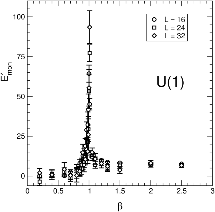
Figure 1: The derivative of the energy to create a monopole ($n_{\text{mon}}=1$), Eq. (33), versus $\beta$ for U(1) lattice gauge theory on a $L^{4}$ lattice (circles refer to $L=16$, squares to $L=24$, and diamonds to $L=32$).

Let us start with the case of the Dirac magnetic monopole background field. In the continuum the magnetic monopole field with the Dirac string in the direction $\vec{n}$ is

$$e\vec{b}({\vec{r}})=\frac{n_{\mathrm{mon}}}{2}\frac{\vec{r}\times\vec{n}}{r(r-\vec{r}\cdot\vec{n})}\,,$$ (30)

where, according to the Dirac quantization condition, $n_{\mathrm{mon}}$ is an integer and $e$ is the electric charge (magnetic charge = $n_{\mathrm{mon}}/2e$). We consider the gauge-invariant background field action Eq. (11) where the external background field is given by the lattice version of the Dirac magnetic monopole field. By choosing $\vec{n}=\hat{x}_{3}$ we get:

$$\begin{split}U^{\text{ext}}_{1,2}(\vec{x})&=\cos[\theta^{\text{mon}}_{1,2}(\vec{x})]+i\sin[\theta^{\text{mon}}_{1,2}(\vec{x})]\,,\\ U^{\text{ext}}_{3}(\vec{x})&={\mathbf{1}}\,,\end{split}$$ (31)

with

$$\begin{split}\theta^{\text{mon}}_{1}(\vec{x})&=-\frac{n_{\text{mon}}}{2}\frac{(x_{2}-X_{2})}{|\vec{x}_{\text{mon}}|}\frac{1}{|\vec{x}_{\text{mon}}|-(x_{3}-X_{3})}\,,\\ \theta^{\text{mon}}_{2}(\vec{x})&=+\frac{n_{\text{mon}}}{2}\frac{(x_{1}-X_{1})}{|\vec{x}_{\text{mon}}|}\frac{1}{|\vec{x}_{\text{mon}}|-(x_{3}-X_{3})}\,.\end{split}$$ (32)

In Equation (32) $(X_{1},X_{2},X_{3})$ are the monopole coordinates and $\vec{x}_{\text{mon}}=(\vec{x}-\vec{X})$. In the numerical simulations we put the lattice Dirac monopole at the center of the time slice $x_{4}=0$. To avoid the singularity due to the Dirac string we locate the monopole between two neighboring sites. We have checked that the numerical results are not too sensitive to the precise position of the magnetic monopole.
To avoid the problem of dealing with a partition function we consider $E^{\prime}_{\mathrm{mon}}=\partial E_{\mathrm{mon}}/\partial\beta$. It is easy to see that $E^{\prime}_{\mathrm{mon}}$ is given by the difference between the average plaquette $<U_{\mu\nu}>$ obtained in turn from configurations without and with the monopole field:

$$E^{\prime}_{\text{mon}}=V\left[<U_{\mu\nu}>_{n_{\text{mon}}=0}-<U_{\mu\nu}>_{n_{\text{mon}}\neq 0}\right]\,,$$ (33)

where $V$ is the spatial volume.

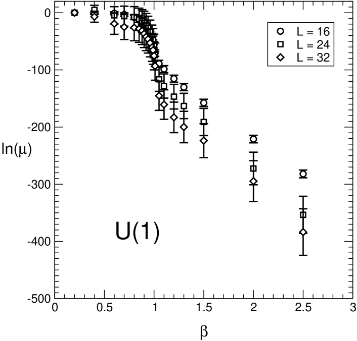
Figure 2: The logarithm of the disorder parameter, Eq. (28), versus $\beta$ for U(1) lattice gauge theory on a $L^{4}$ lattice. Symbols as in Fig. 1.

We performed lattice simulations on $16^{4}$, $24^{4}$ and $32^{4}$ lattices using an APE100 computer. The spatial links belonging to the time slice $x_{4}=0$ and to the spatial boundaries of the other time slices ($x_{4}\neq 0$) are constrained, therefore they are not updated during Monte Carlo simulation. Therefore we must consider only the “dynamical links” in the computation of $E^{\prime}_{\text{mon}}$. This means that the generic plaquette $U_{\mu\nu}(x)=U_{\mu}(x)U_{\nu}(x+\hat{\mu})U^{\dagger}_{\mu}(x+\hat{\nu})U^{\dagger}_{\nu}(x)$ contributes to Eq. (33) if the link $U_{\mu}(x)$ is a ”dynamical” one (i.e. it is not constrained in the lattice Schrod̈inger functional integration).
Since we are measuring a local quantity such as average plaquette $<U_{\mu\nu}>$ , a low statistics (from 1000 up to 5000 configurations) is required in order to get a good estimate of $E^{\prime}_{\mathrm{mon}}$. Statistical errors have been estimated using the jackknife resampling method [50, 51], modified to take into account the statistical correlations between lattice configurations.
In Fig. 1 we report our numerical results for $E^{\prime}_{\mathrm{mon}}$ versus $\beta$ for three different lattice sizes.

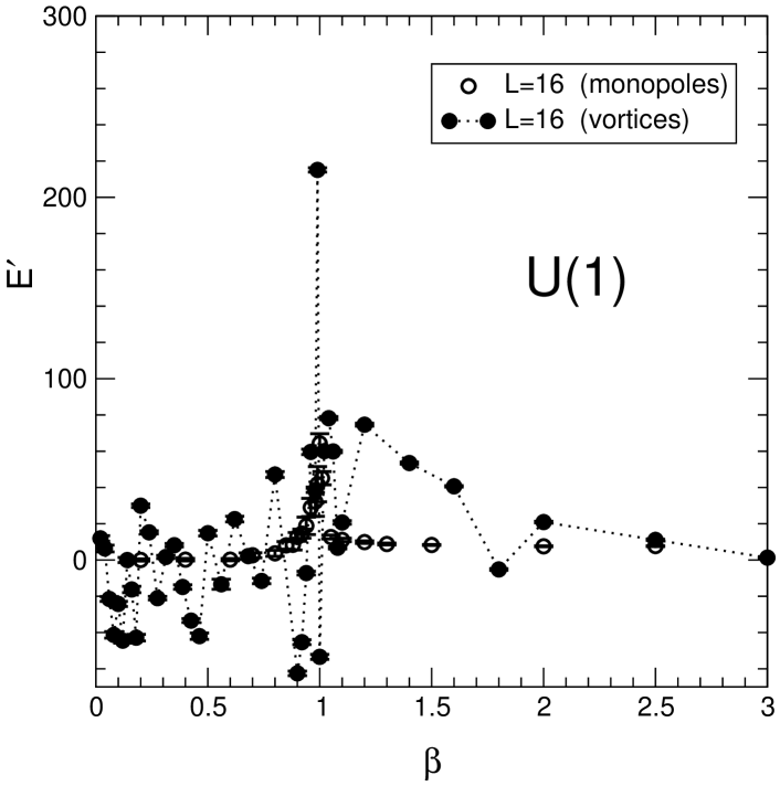
Figure 3: The derivative of the energy to create a monopole or a vortex versus $\beta$ for U(1) lattice gauge theory on a $16^{4}$ lattice. Open circles refer to a monopole background field ($n_{\text{mon}}=1$) and full circles to a vortex background field ($n_{\text{vort}}=1$) .

We see that in strong coupling region ($\beta\lesssim 1$), monopole internal energy derivative is zero, insensitive to the lattice size. This means that, according to Eq. (28), the disorder parameter $\mu\simeq 1$. On the other hand, near the critical coupling $\beta_{c}\simeq 1$, $E^{\prime}_{\mathrm{mon}}$ displays a sharp peak which increases by increasing the lattice volume. In the weak coupling region ($\beta\gg\beta_{c}$) the plateau in $E^{\prime}_{\mathrm{mon}}$ indicates that the monopole energy tends to the classical monopole action which behaves linearly in $\beta$.
In order to obtain $\mu$ we perform the numerical integration of $E^{\prime}_{\mathrm{mon}}$

$$E_{{\mathrm{mon}}}=\int_{0}^{\beta}E^{\prime}_{\mathrm{mon}}\,d\beta^{\prime}$$ (34)

In Fig. 2 we display the logarithm of the disorder parameter $\mu$ versus $\beta$. In the confined phase we see that $\ln\mu=0$, so that Eq. (28) tells us that the energy required to create a monopole is zero and therefore monopoles condense in the confined U(1) vacuum. Correspondingly the disorder parameter $\mu$ is different from zero in the confined phase. Moreover numerical data suggest that $\mu\to 0$ when $\beta\to\beta_{c}$ in the thermodynamic limit. Note that the different curves for $\mu$ corresponding to increasing lattice sizes seem to cross, suggesting a first order phase transition. However, in order to extract the critical parameters and to determine the order of transition we need to perform a finite size scaling analysis, which will be addressed in a future work.

Let us now consider the case of U(1) magnetic vortices. The continuum gauge potential for a classical magnetic vortex along the $x_{3}$-direction with $n_{\text{vort}}$ units of elementary flux $\phi=2\pi/e$ is given by

$$\begin{split}A^{\text{ext}}_{1}&=-\frac{n_{\text{vort}}}{e}\frac{x_{2}}{(x_{1})^{2}+(x_{2})^{2}}\,,\\ A^{\text{ext}}_{2}&=\frac{n_{\text{vort}}}{e}\frac{x_{1}}{(x_{1})^{2}+(x_{2})^{2}}\,,\\ A^{\text{ext}}_{3}&=0\,.\end{split}$$ (35)

The corresponding lattice links are:

$$\begin{split}U^{\text{ext}}_{1,2}(\vec{x})&=\cos[\theta^{\text{vort}}_{1,2}(\vec{x})]+i\sin[\theta^{\text{vort}}_{1,2}(\vec{x})]\,,\\ \theta^{\text{vort}}_{1,2}&=\mp\,n_{\text{vort}}\,\frac{x_{2,1}}{(x_{1})^{2}+(x_{2})^{2}}\,,\\ U^{\text{ext}}_{3}(\vec{x})&=\mathbf{1}\,.\end{split}$$ (36)

As in the monopole case we evaluated numerically the $\beta$-derivative, $E^{\prime}_{\mathrm{vort}}$, of the energy to create a vortex. In Fig. 3 we compare the monopole and vortex energy derivative for a $16^{4}$ lattice . While we clearly see that in the strong coupling monopoles condense, the $\beta$-derivative of the vortex energy displays rapid oscillations whose amplitude seems to increase near the critical coupling. This means that we cannot obtain a reliable estimate of $E_{\mathrm{vort}}$ by a numerical integration of $E^{\prime}_{\mathrm{vort}}$. However, we can safely say that our data do not show any signal of vortex condensation which would imply that $E^{\prime}_{\text{vort}}=0$ at strong couplings.
Thus, we may conclude that in U(1) lattice theory the strong coupling confined phase is intimately related to magnetic monopole condensation.

3 SU(2)

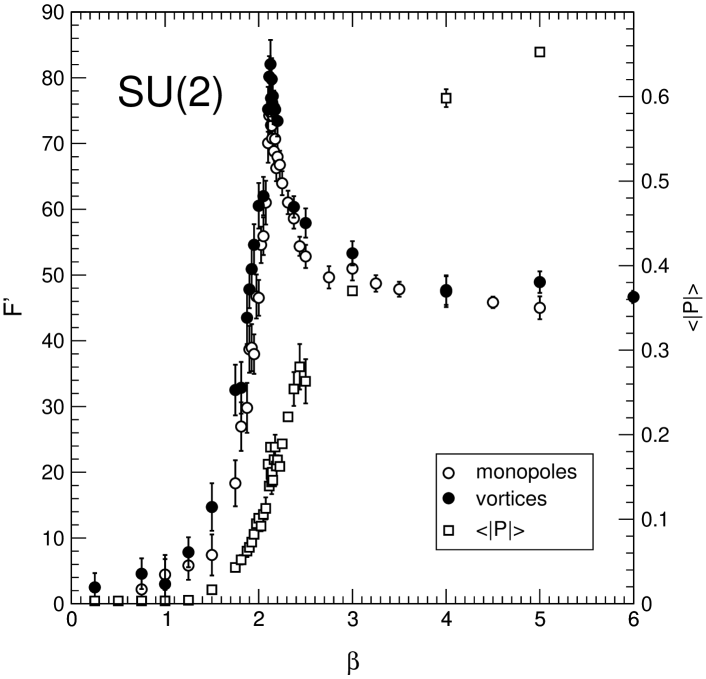
Figure 4: The derivative of the free energy, Eq. (41), versus $\beta$ for monopoles (open circles) and vortices (full circles) for SU(2) on a $24^{3}\times 4$ lattice. The absolute value of the Polyakov loop, Eq. (43), is also displayed (open squares).

In a previous work [7] we studied Abelian magnetic monopole condensation in finite temperature SU(2) lattice gauge theory. For SU(2) the maximal Abelian group is an Abelian U(1) group. In the continuum the Abelian monopole field is given by

$$g\vec{b}^{a}({\vec{x}})=\delta^{a,3}\frac{n_{\mathrm{mon}}}{2}\frac{\vec{x}\times\vec{n}}{|\vec{x}|(|\vec{x}|-\vec{x}\cdot\vec{n})}\,,$$ (37)

where $\vec{n}$ is the direction of the Dirac string and, according to the Dirac quantization condition, $n_{\text{mon}}$ is an integer. The lattice links corresponding to the Abelian monopole field Eq. (37) can be readily obtained from Eq. (6). By choosing $\vec{n}=\hat{x}_{3}$ we have:

$$\begin{split}U^{\text{ext}}_{1,2}(\vec{x})&=\cos[\theta^{\text{mon}}_{1,2}(\vec{x})]+i\sigma_{3}\sin[\theta^{\text{mon}}_{1,2}(\vec{x})]\,,\\ U^{\text{ext}}_{3}(\vec{x})&={\mathbf{1}}\,,\end{split}$$ (38)

with

$$\begin{split}\theta^{\text{mon}}_{1}(\vec{x})&=-\frac{n_{\text{mon}}}{4}\frac{(x_{2}-X_{2})}{|\vec{x}_{\text{mon}}|}\frac{1}{|\vec{x}_{\text{mon}}|-(x_{3}-X_{3})}\,,\\ \theta^{\text{mon}}_{2}(\vec{x})&=+\frac{n_{\text{mon}}}{4}\frac{(x_{1}-X_{1})}{|\vec{x}_{\text{mon}}|}\frac{1}{|\vec{x}_{\text{mon}}|-(x_{3}-X_{3})}\,,\end{split}$$ (39)

where $(X_{1},X_{2},X_{3})$ are the monopole coordinates, $\vec{x}_{\text{mon}}=(\vec{x}-\vec{X})$ and the $\sigma_{a}$’s are the Pauli matrices.

As discussed in Sect. 1, at finite temperature the disorder parameter, Eq. (29), is defined by means of the thermal partition function $\mathcal{Z}_{T}[A^{\text{ext}}]$ in presence of the Abelian monopole background field Eq. (37). Numerical results in Ref. [7] show that the monopole disorder parameter $\mu$ is different from zero in the confined phase and suggest that it tends to zero when approaching the critical coupling in the thermodynamic limit. Thus SU(2) confining vacuum does display the Abelian monopole condensation in accordance with dual superconductivity hypothesis.

Now we want discuss what happens if we consider an Abelian vortex background field. In SU(2) gauge theory, Abelian vortex field on the lattice is given by

$$\begin{split}U^{\text{ext}}_{1,2}(\vec{x})&=\cos[\theta^{\text{vort}}_{1,2}(\vec{x})]+i\sigma_{3}\sin[\theta^{\text{vort}}_{1,2}(\vec{x})]\,,\\ U^{\text{ext}}_{3}(\vec{x})&={\mathbf{1}}\,,\\ \theta^{\text{vort}}_{1,2}(\vec{x})&=\mp\frac{n_{\text{vort}}}{2}\frac{x_{2,1}}{(x_{1})^{2}+(x_{2})^{2}}\,.\end{split}$$ (40)

Again, the derivative of the free energy required to create a vortex

$$F^{\prime}_{\text{vort}}=\frac{\partial}{\partial\beta}F_{\text{vort}}\,,$$ (41)

can be easily evaluated as the difference between the average plaquette $<U_{\mu\nu}>$ without the vortex background field (i.e. $n_{\text{vort}}=0$) and with the vortex background field ($n_{\text{vort}}\neq 0$)

$$F^{\prime}_{\text{vort}}=V\left[<U_{\mu\nu}>_{n_{\text{vort}}=0}-<U_{\mu\nu}>_{n_{\text{vort}}\neq 0}\right]\,,$$ (42)

where $V$ is the spatial volume. In Eq. (42) we include only the contributions due to the dynamical links (see discussion after Eq. (33)).

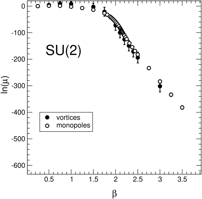
Figure 5: The logarithm of the disorder parameter, Eq. (29), versus $\beta$ for vortices (full circles) and monopoles (open circles). Data refer to SU(2) gauge theory on a $24^{3}\times 4$ lattice.

A low statistics (from 2000 up to 10000 configurations) is required in order to get a good estimate of the derivative of the free energy. In Fig. 4 we display the derivative of the vortex free energy versus $\beta$ for $n_{\text{vort}}=10$ on lattices with $L_{t}=4$ and $L_{s}=24$. We see that $F^{\prime}_{\text{vort}}$ vanishes at strong coupling and displays a rather sharp peak near $\beta\backsimeq 2.2$. We expect that this peak corresponds to the finite temperature deconfinement transition. In Fig. 4 we also display the absolute value of the Polyakov loop in time direction

$$P=\frac{1}{V}\sum_{\vec{x}}\frac{1}{2}{\text{Tr}}\prod_{x_{4}=1}^{L_{t}}U_{4}(x_{4},\vec{x})$$ (43)

and, indeed, we can see that the peak in $F^{\prime}_{\text{vort}}$ corresponds to the rise of the Polyakov loop.
In weak coupling region the plateau in $F^{\prime}_{\text{vort}}$ indicates that vortex free energy tends to the classical vortex action which behaves linearly in $\beta$.

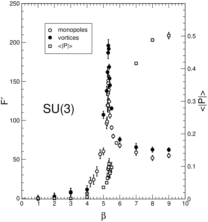
Figure 6: The derivative of the free energy versus $\beta$ for monopoles (open circles) and vortices (full circles). The absolute value of the Polyakov loop, Eq. (51), is also displayed (open squares). Data refer to SU(3) gauge theory on a $32^{3}\times 4$ lattice.

In Fig. 4 we display for comparison also the derivative of the Abelian monopole free energy for $n_{\text{mon}}=10$. It turns out that monopoles and vortices data agree within statistical errors. To appreciate better this last point we plotted in Fig. 5 the logarithm of the disorder parameter Eq. (29) for monopoles and vortices respectively. Fig. 5 shows clearly that monopoles and vortices agree quite perfectly. Our results strongly suggest that also Abelian vortices could play a role in the dynamics of confinement.

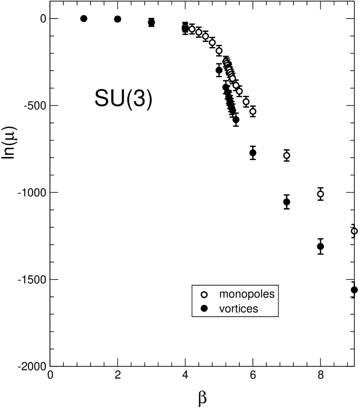
Figure 7: The logarithm of the disorder parameter, Eq. (29), versus $\beta$ for $T_{8}$ monopoles (open circles) and $T_{8}$ vortices (full circles). Data refer to SU(3) gauge theory on a $32^{3}\times 4$ lattice.

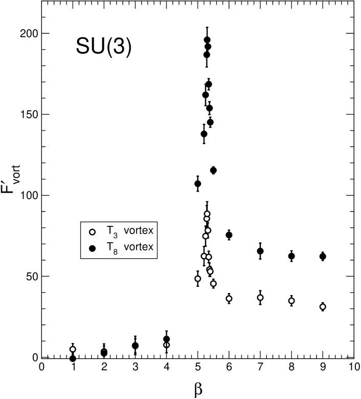
Figure 8: The free energy derivative for $T_{3}$ vortices (open circles) and $T_{8}$ vortices (full circles) versus $\beta$. Data refer to SU(3) gauge theory on a $32^{3}\times 4$ lattice.

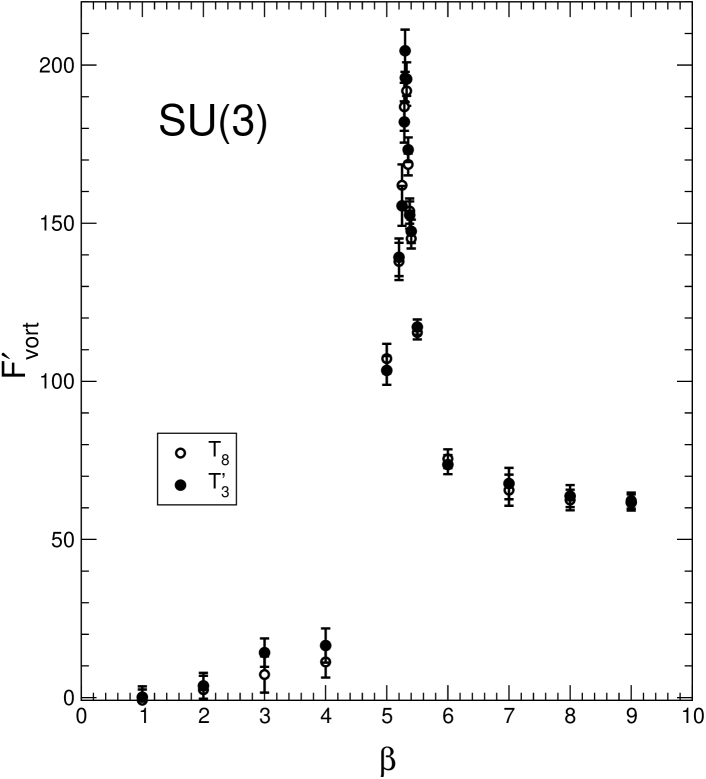
Figure 9: The free energy derivative for $T_{8}$ vortices (open circles) and $T^{\prime}_{3}$ vortices (full circles) versus $\beta$. Data refer to SU(3) gauge theory on a $32^{3}\times 4$ lattice.

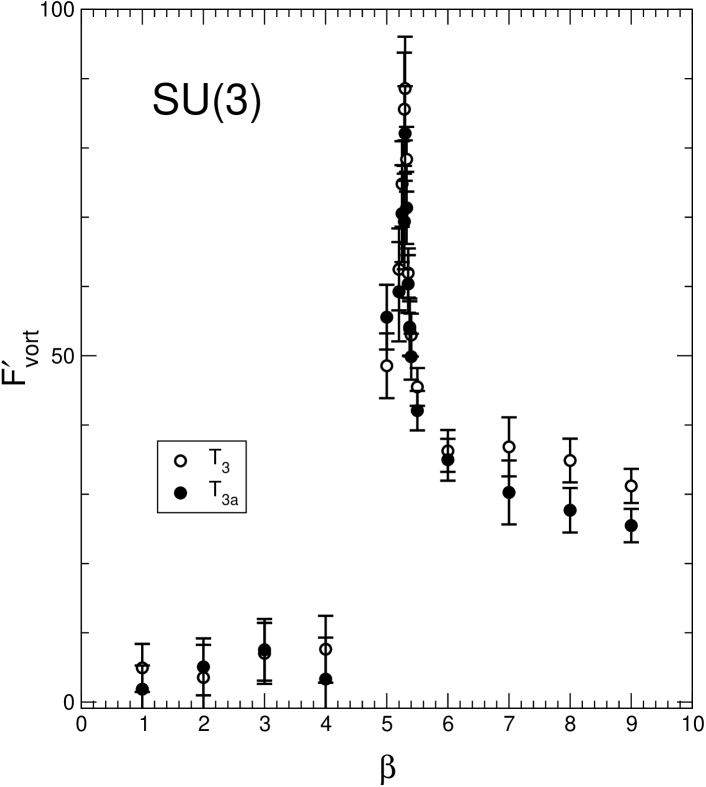
Figure 10: The free energy derivative for $T_{3}$ vortices (open circles) and $T_{3a}$ vortices (full circles) versus $\beta$. Data refer to SU(3) gauge theory on a $32^{3}\times 4$ lattice.

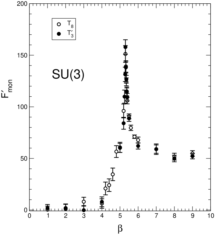
Figure 11: The free energy derivative for $T_{8}$ monopoles (open circles) and $T^{\prime}_{3}$ monopoles (full circles) versus $\beta$. Data refer to SU(3) gauge theory on a $32^{3}\times 4$ lattice.

4 SU(3)

For SU(3) gauge theory the maximal Abelian group is U(1)$\times$U(1), therefore we may introduce two independent types of Abelian monopoles or Abelian vortices.

Let us consider the Abelian monopole field. The first type of Abelian monopole field is derived considering the $\lambda_{3}$ diagonal generator, we name it $T_{3}$ Abelian monopole (following Ref. [7]). On the lattice it is given by

$$\begin{split}U_{1,2}^{\text{ext}}(\vec{x})&=\begin{bmatrix}e^{i\theta^{\text{mon}}_{1,2}(\vec{x})}&0&0\\ 0&e^{-i\theta^{\text{mon}}_{1,2}(\vec{x})}&0\\ 0&0&1\end{bmatrix}\,\\ U^{\text{ext}}_{3}(\vec{x})&={\mathbf{1}}\,,\end{split}$$ (44)

with $\theta^{\text{mon}}_{1,2}(\vec{x})$ defined in Eq. (39).
The second type of independent Abelian monopole can be obtained by considering the diagonal generator $\lambda_{8}$. In this case we have the $T_{8}$ Abelian monopole:

$$\begin{split}U_{1,2}^{\text{ext}}(\vec{x})&=\begin{bmatrix}e^{i\theta^{\text{mon}}_{1,2}(\vec{x})}&0&0\\ 0&e^{i\theta^{\text{mon}}_{1,2}(\vec{x})}&0\\ 0&0&e^{-2i\theta^{\text{mon}}_{1,2}(\vec{x})}\end{bmatrix}\,\\ U^{\text{ext}}_{3}(\vec{x})&={\mathbf{1}}\;\,,\end{split}$$ (45)

with

$$\begin{split}\theta^{\text{mon}}_{1}(\vec{x})&=\frac{1}{\sqrt{3}}\left[-\frac{n_{\text{mon}}}{4}\frac{(x_{2}-X_{2})}{|\vec{x}_{\text{mon}}|}\frac{1}{|\vec{x}_{\text{mon}}|-(x_{3}-X_{3})}\right]\,,\\ \theta^{\text{mon}}_{2}(\vec{x})&=\frac{1}{\sqrt{3}}\left[+\frac{n_{\text{mon}}}{4}\frac{(x_{1}-X_{1})}{|\vec{x}_{\text{mon}}|}\frac{1}{|\vec{x}_{\text{mon}}|-(x_{3}-X_{3})}\right]\,.\end{split}$$ (46)

Analogously, we have the $T_{3}$ Abelian vortex:

$$\begin{split}U_{1,2}^{\text{ext}}(\vec{x})&=\begin{bmatrix}e^{i\theta^{\text{vort}}_{1,2}(\vec{x})}&0&0\\ 0&e^{-i\theta^{\text{vort}}_{1,2}(\vec{x})}&0\\ 0&0&1\end{bmatrix}\,,\\[8.5359pt] U_{3}^{\text{ext}}(\vec{x})&={\mathbf{1}}\\[8.5359pt] \theta^{\text{vort}}_{1,2}&=\mp\frac{n_{\text{vort}}}{2}\frac{x_{2,1}}{(x_{1})^{2}+(x_{2})^{2}}\;\;.\end{split}$$ (47)

and the $T_{8}$ Abelian vortex:

$$\begin{split}U_{1,2}^{\text{ext}}(\vec{x})&=\begin{bmatrix}e^{i\theta^{\text{vort}}_{1,2}(\vec{x})}&0&0\\ 0&e^{i\theta^{\text{vort}}_{1,2}(\vec{x})}&0\\ 0&0&e^{-2i\theta^{\text{vort}}_{1,2}(\vec{x})}\end{bmatrix}\,,\\[8.5359pt] U_{3}^{\text{ext}}(\vec{x})&={\mathbf{1}}\\[8.5359pt] \theta^{\text{vort}}_{1,2}&=\mp\frac{1}{\sqrt{3}}\frac{n_{\text{vort}}}{2}\frac{x_{2,1}}{(x_{1})^{2}+(x_{2})^{2}}\;\;,\end{split}$$ (48)

Other Abelian monopoles and vortices can be generated by considering linear combinations of $\lambda_{3}$ and $\lambda_{8}$ generators. In particular we have also considered the following two linear combinations of $\lambda_{3}/2$ and $\lambda_{8}/2$

$$T_{3a}=-\frac{1}{2}\frac{\lambda_{3}}{2}+\frac{\sqrt{3}}{2}\frac{\lambda_{8}}{2}=\begin{bmatrix}0&0&0\\ 0&\frac{1}{2}&0\\ 0&0&-\frac{1}{2}\end{bmatrix}\,,$$ (49)

and

$$T^{\prime}_{3}=\frac{\sqrt{3}}{2}\frac{\lambda_{3}}{2}+\frac{1}{2}\frac{\lambda_{8}}{2}=\begin{bmatrix}\frac{1}{\sqrt{3}}&0&0\\ 0&-\frac{1}{2\sqrt{3}}&0\\ 0&0&-\frac{1}{2\sqrt{3}}\end{bmatrix}\,.$$ (50)

The linear combinations given in Eq. (49) and in Eq. (50) have been also considered in Ref. [4, 5] and in Ref. [25] respectively.

For reader convenience, let us summarize the main results of our previous investigation of Abelian monopole condensation [7] in SU(3). In Ref. [7] we found that there is condensation of Abelian monopoles in the non-perturbative vacuum and that SU(3) vacuum reacts moderately strongly in the case of the $T_{8}$ Abelian monopole (in particular the peak value of $F^{\prime}_{\text{mon}}$ for $T_{8}$ Abelian monopoles is about two times higher than the corresponding peak for $T_{3}$ Abelian monopoles).

In the present paper we compare $T_{8}$ Abelian monopoles and vortices. In Fig. 6 the free energy derivative for monopoles (with $n_{\text{mon}}=10$) and vortices (with $n_{\text{vort}}=10$) is displayed versus $\beta$ for a lattice with $L_{s}=32$ and $L_{t}=4$. We also display the absolute value of the Polyakov loop in the time direction

$$P=\frac{1}{V}\sum_{\vec{x}}\frac{1}{3}{\text{Tr}}\prod_{x_{4}=1}^{L_{t}}U_{4}(x_{4},\vec{x})\,.$$ (51)

As can be argued from Fig. 6, $F^{\prime}_{\text{vort}}$ behaves like $F^{\prime}_{\text{mon}}$. Indeed, the free energy derivatives are zero within errors in the strong coupling region and display a sharp peak in correspondence of the rise of the Polyakov loop. In the weak coupling region the free energy derivatives are almost constant. The values of the plateau correspond to the beta derivative of the lattice classical action. Remarkably Fig. 6 shows that in the peak region the $T_{8}$ Abelian vortex displays a signal higher than the Abelian monopole. This is better appreciated if we look at the disorder parameter Eq. (29) (see Fig. 7), where $\ln\mu$ for Abelian vortices has a sizeable faster decrease. In the study of Abelian monopole condensation we found [7] that the color direction $\hat{8}$ is slightly preferred with respect to the direction $\hat{3}$ in the color space. It is worthwhile to see if this result holds also for Abelian vortex condensation. In Fig. 8 we compare the free energy derivative for the $T_{3}$ and $T_{8}$ Abelian vortices for the lattice with $L_{t}=4$ and $L_{s}=32$. As expected the $T_{8}$ Abelian vortex displays, in the peak region, a signal about a factor two higher.

Finally in Fig. 9 and in Fig. 10 we confront the $T_{3}$, $T_{3a}$, $T_{8}$ and $T^{\prime}_{3}$ Abelian vortices. We find that $T_{3}$ and $T_{8}$ agree within statistical errors in the whole range of $\beta$ with $T_{3a}$ and $T^{\prime}_{3}$ respectively. For the sake of completeness, in Fig. 11 we compare $T^{\prime}_{3}$ and $T_{8}$ monopoles, showing that they agree within statistical errors.

We may conclude that, even for SU(3) gauge theory, our results strongly suggest that Abelian vortices play a role in the dynamics of confinement.

5 Conclusions

We investigated Abelian monopole and Abelian vortex condensation in U(1), SU(2) and SU(3) lattice gauge theories.
For U(1) pure lattice gauge theory we found that, in the confined phase, the vacuum can be interpreted as a coherent condensate of magnetic monopoles. On the other hand, we do not find convincing evidence of condensation of vortices.
For non Abelian SU(2) and SU(3) lattice gauge theories at finite temperature, by means of a lattice thermal partition functional, we introduced a disorder parameter for detecting Abelian monopole and Abelian vortex condensation in the confined phase. The disorder parameter is defined by means of a lattice thermal partition functional and is invariant for gauge transformations of the external background (monopole or vortex) field.

Our numerical results suggest that the disorder parameter for both Abelian monopoles and Abelian vortices is different from zero in the confined phase and tends to zero when approaching the critical coupling in the thermodynamic limit. Therefore in SU(2) and SU(3) Abelian vortices could play a role in the dynamics of confinement.
In particular for SU(2) gauge theory there is also a quantitative agreement between the measured values of free energies for monopoles and vortices.
On the other hand, remarkably, in SU(3) gauge theory it turns out that the Abelian vortex displays a signal higher than the Abelian monopole. Moreover, for the Abelian vortices we find that the non perturbative vacuum reacts moderately strongly to $T_{8}$ vortices with respect to $T_{3}$ vortices. This last point is in accordance with our finding in the study of SU(3) Abelian monopole condensation [7].

In conclusion it is worthwhile to observe that our results point to a different mechanism of confinement for U(1) lattice gauge theory with respect to SU(2) and SU(3) gauge theories. Indeed, in the U(1) Abelian case we find that the confining vacuum behaves as a coherent condensate of Dirac magnetic monopoles. In SU(2) and SU(3) it seems that there is condensation of Abelian magnetic monopoles and Abelian vortices. So that in SU(2) and SU(3) gauge theories one could look at the confining vacuum as a coherent Abelian magnetic condensate. Even more, for the SU(3) theory, it turns out that gauge field configurations leading to Abelian magnetic flux tubes, multiple of the elementary flux, seem to be favorite with respect to Abelian magnetic monopoles.

We would like to remark that it is important to perform a finite size scaling analysis both for SU(2) and SU(3). Indeed a finite size scaling analysis will allow us to determine the critical behavior of the disorder parameter in the thermodynamic limit.

We stress finally, that it should be interesting to extend our method to study center vortex condensation in SU(2) and SU(3) lattice gauge theories. First results in this direction have been reported in Ref. [52].

References

- [1] G. ’t Hooft, The confinement phenomenon in quantum field theory, in High Energy Physics, EPS International Conference, Palermo, 1975.
- [2] S. Mandelstam, Vortices and quark confinement in non Abelian gauge theories, Phys. Rept. 23 (1976) 245.
- [3] A. Di Giacomo, Mechanisms of color confinement, Acta Phys. Polon. B25 (1994) 215–226.
- [4] A. Di Giacomo, B. Lucini, L. Montesi, and G. Paffuti, Colour confinement and dual superconductivity of the vacuum. i, Phys. Rev. D61 (2000) 034503, [hep-lat/9906024].
- [5] A. Di Giacomo, B. Lucini, L. Montesi, and G. Paffuti, Colour confinement and dual superconductivity of the vacuum. ii, Phys. Rev. D61 (2000) 034504, [hep-lat/9906025].
- [6] J. M. Carmona, M. D’Elia, A. Di Giacomo, B. Lucini, and G. Paffuti, Color confinement and dual superconductivity of the vacuum. iii, hep-lat/0103005.
- [7] P. Cea and L. Cosmai, Gauge invariant study of the monopole condensation in non Abelian lattice gauge theories, Phys. Rev. D62 (2000) 094510, [hep-lat/0006007].
- [8] H. Shiba and T. Suzuki, Monopole action and condensation in SU(2) QCD, Phys. Lett. B351 (1995) 519–527, [hep-lat/9408004].
- [9] N. Arasaki, S. Ejiri, S.-i. Kitahara, Y. Matsubara, and T. Suzuki, Monopole action and monopole condensation in SU(3) lattice QCD, Phys. Lett. B395 (1997) 275–282, [hep-lat/9608129].
- [10] N. Nakamura et. al., Disorder parameter of confinement, Nucl. Phys. Proc. Suppl. 53 (1997) 512–514, [hep-lat/9608004].
- [11] M. N. Chernodub, M. I. Polikarpov, and A. I. Veselov, Effective constraint potential for Abelian monopole in SU(2) lattice gauge theory, Phys. Lett. B399 (1997) 267–273, [hep-lat/9610007].
- [12] J. Jersak, T. Neuhaus, and H. Pfeiffer, Scaling analysis of the magnetic monopole mass and condensate in the pure U(1) lattice gauge theory, Phys. Rev. D60 (1999) 054502, [hep-lat/9903034].
- [13] C. Hoelbling, C. Rebbi, and V. A. Rubakov, Free energy of an SU(2) monopole-antimonopole pair, Phys. Rev. D63 (2001) 034506, [hep-lat/0003010].
- [14] M. Faber, J. Greensite, S. Olejnik, and D. Yamada, The vortex-finding property of maximal center (and other) gauges, JHEP 12 (1999) 012, [hep-lat/9910033].
- [15] K. Langfeld, O. Tennert, M. Engelhardt, and H. Reinhardt, Center vortices of Yang-Mills theory at finite temperatures, Phys. Lett. B452 (1999) 301, [hep-lat/9805002].
- [16] P. de Forcrand and M. D’Elia, On the relevance of center vortices to QCD, Phys. Rev. Lett. 82 (1999) 4582–4585, [hep-lat/9901020].
- [17] R. Bertle, M. Faber, J. Greensite, and S. Olejnik, The structure of projected center vortices at zero and finite temperature, Nucl. Phys. Proc. Suppl. 83 (2000) 425–427, [hep-lat/9909002].
- [18] J. Ambjorn, J. Giedt, and J. Greensite, Vortex structure vs. monopole dominance in Abelian projected gauge theory, JHEP 02 (2000) 033, [hep-lat/9907021].
- [19] A. Montero, SU(3) vortex-like configurations in the maximal center gauge, Nucl. Phys. Proc. Suppl. 83 (2000) 518–520, [hep-lat/9907024].
- [20] O. Jahn, F. Lenz, J. W. Negele, and M. Thies, Center vortices, instantons, and confinement, Nucl. Phys. Proc. Suppl. 83 (2000) 524–526, [hep-lat/9909062].
- [21] J. D. Stack and W. Tucker, On the distribution of vortex sizes and the long range potential, Nucl. Phys. Proc. Suppl. 83 (2000) 539–540.
- [22] B. L. G. Bakker, A. I. Veselov, and M. A. Zubkov, Central dominance and the confinement mechanism in gluodynamics, Phys. Lett. B471 (1999) 214–219, [hep-lat/9902010].
- [23] A. Alexandru and R. W. Haymaker, Vortices in SO(3) Z(2) simulations, Nucl. Phys. Proc. Suppl. 94 (2001) 475–477, [hep-lat/0009012].
- [24] L. Del Debbio, A. Di Giacomo, and B. Lucini, Vortices, monopoles and confinement, Nucl. Phys. B594 (2001) 287–300, [hep-lat/0006028].
- [25] P. de Forcrand and M. Pepe, Center vortices and monopoles without lattice Gribov copies, Nucl. Phys. B598 (2001) 557–577, [hep-lat/0008016].
- [26] T. G. Kovacs and E. T. Tomboulis, Computation of the vortex free energy in SU(2) gauge theory, Phys. Rev. Lett. 85 (2000) 704–707, [hep-lat/0002004].
- [27] C. Korthals-Altes and A. Kovner, Magnetic Z(N) symmetry in hot QCD and the spatial Wilson loop, Phys. Rev. D62 (2000) 096008, [hep-ph/0004052].
- [28] G. ’t Hooft, On the phase transition towards permanent quark confinement, Nucl. Phys. B138 (1978) 1.
- [29] J. M. Cornwall, Quark confinement and vortices in massive gauge invariant QCD, Nucl. Phys. B157 (1979) 392.
- [30] J. M. Cornwall, Center vortices and confinement vs. screening, Phys. Rev. D57 (1998) 7589–7600, [hep-th/9712248].
- [31] L. G. Yaffe, Confinement in SU(N) lattice gauge theories, Phys. Rev. D21 (1980) 1574.
- [32] G. Mack and V. B. Petkova, Comparison of lattice gauge theories with gauge groups Z(2) and SU(2), Ann. Phys. 123 (1979) 442.
- [33] G. Mack and V. B. Petkova, Sufficient condition for confinement of static quarks by a vortex condensation mechanism, Ann. Phys. 125 (1980) 117.
- [34] E. Tomboulis, The ’t Hooft loop in SU(2) lattice gauge theories, Phys. Rev. D23 (1981) 2371.
- [35] E. T. Tomboulis, Confinement via dynamical monopoles, Phys. Lett. B303 (1993) 103–108.
- [36] P. Cea and L. Cosmai, Magnetic condensation and confinement in lattice gauge theory, Nucl. Phys. Proc. Suppl. 94 (2001) 486–489, [hep-lat/0010034].
- [37] L. P. Kadanoff and H. Ceva, Determination of an opeator algebra for the two-dimensional Ising model, Phys. Rev. B3 (1971) 3918–3938.
- [38] E. H. Fradkin and L. Susskind, Order and disorder in gauge systems and magnets, Phys. Rev. D17 (1978) 2637.
- [39] A. C. Davis, T. W. B. Kibble, A. Rajantie, and H. Shanahan, Topological defects in lattice gauge theories, JHEP 11 (2000) 010, [hep-lat/0009037].
- [40] P. Cea, L. Cosmai, and A. D. Polosa, The lattice Schrödinger functional and the background field effective action, Phys. Lett. B392 (1997) 177–181, [hep-lat/9601010].
- [41] P. Cea and L. Cosmai, Lattice background effective action: A proposal, Nucl. Phys. Proc. Suppl. 53 (1997) 574–577, [hep-lat/9607015].
- [42] P. Cea and L. Cosmai, Probing the non-perturbative dynamics of SU(2) vacuum, Phys. Rev. D60 (1999) 094506, [hep-lat/9903005].
- [43] M. Lüscher, R. Narayanan, P. Weisz, and U. Wolff, The Schrödinger functional: A renormalizable probe for non Abelian gauge theories, Nucl. Phys. B384 (1992) 168–228, [hep-lat/9207009].
- [44] M. Lüscher and P. Weisz, Background field technique and renormalization in lattice gauge theory, Nucl. Phys. B452 (1995) 213–233, [hep-lat/9504006].
- [45] S. Sint, On the Schrödinger functional in QCD, Nucl. Phys. B421 (1994) 135–158, [hep-lat/9312079].
- [46] M. Luscher, R. Sommer, U. Wolff, and P. Weisz, Computation of the running coupling in the SU(2) Yang-Mills theory, Nucl. Phys. B389 (1993) 247–264, [hep-lat/9207010].
- [47] G. C. Rossi and M. Testa, The structure of Yang-Mills theories in the temporal gauge. 1. general formulation, Nucl. Phys. B163 (1980) 109.
- [48] G. C. Rossi and M. Testa, The structure of Yang-Mills theories in the temporal gauge. 2. perturbation theory, Nucl. Phys. B176 (1980) 477.
- [49] D. J. Gross, R. D. Pisarski, and L. G. Yaffe, QCD and instantons at finite temperature, Rev. Mod. Phys. 53 (1981) 43.
- [50] B. Efron, Jackknife, the Bootstrap and Other Resampling Plans. SIAM Press, Philadelphia, 1982.
- [51] J. Shao and D. Tu, The Jackknife and the Bootstrap. Springer, New York, 1995.
- [52] P. Cea and L. Cosmai, Abelian and center vortex condensation in SU(3) lattice gauge theory, hep-lat/0110002.