${\rm CP}^{N-1}$ Models with a $\theta$ Term and Fixed Point Action

1 Introduction

It is interesting to study the phase structure of asymptotic free theories such as QCD and the ${\rm CP}^{N-1}$ model. Non-perturbative studies of the phase structure of such theories are necessary in order to understand why effects of the topological term ($\theta$ term) are suppressed in Nature. The $\theta$ term affects the dynamics at low energy and is expected to lead to rich phase structures. [1] Actually, in the Z(N) gauge model, it has been shown by use of free energy arguments that oblique confinement phases could emerge and that an interesting phase structure may be realized. [2] In this paper we are concerned with the dynamics of the $\theta$ vacuum of ${\rm CP}^{N-1}$ models with a topological term, which have several dynamical properties in common with QCD. We believe that study of the two-dimensional model will be useful in acquiring information about realistic physics.

From the numerical point of view, the topological term introduces a complex Boltzmann weight in the Euclidean lattice path integral formalism. The complex nature of the weight prevents one from straightforwardly applying the standard algorithm used for Monte Carlo simulations. This problem can be circumvented by Fourier-transforming the topological charge distribution $P(Q)$. [3, 4] It is then necessary to calculate $P(Q)$ as precisely as possible in order to reduce errors in the expectation values of physical operators as functions of $\theta$. The precise determination of $P(Q)$ will allow us to obtain a partition function and other quantities as functions of $\theta$ with high precision.

It is non-trivial how lattice cut-off effects would emerge through the introduction of a topological term. In the present paper, we employ fixed point (FP) actions to study this issue. [5] In the case of no topological term, the FP action is known to significantly suppress lattice cut-off effects for topological objects in ${\rm CP}^{N-1}$ models. [6, 7, 8] In Ref.[7], a FP action for the ${\rm CP}^{1}$ model (${\rm CP}^{1}$FP) was determined, and the stability of instantons under minimization of the action was investigated in detail. It was also observed there that dislocations can be eliminated by adopting a FP charge as well as the FP action. However, the scaling behavior of the lattice topological susceptibility $\chi_{t}$ was found to be strongly violated even after the dislocations are eliminated. For the ${\rm CP}^{3}$ model with an FP action (${\rm CP}^{3}$FP), contrastingly, impressive improvements have been found; [8] after the topological defects are removed, clear scaling behavior of $\chi_{t}$ is observed.

In the present paper, we study the topological terms of ${\rm CP}^{3}$ and ${\rm CP}^{1}$ models with a FP action. For comparison, we also carry out a calculation for the ${\rm CP}^{3}$ model with the standard action (${\rm CP}^{3}$ST). The main purposes of the paper are the followings.

1. To study the scaling behavior of various quantities such as $P(Q)$, the free energy, the expectation value of the topological charge, the topological susceptibility, and correlation length as a function of $Q$.

2. To analyze $P(Q)$ in detail by considering an effective power $\gamma_{\it eff}$ of $\ln P(Q)$.

The second of these purposes is associated with the phase structure of the model. In the very strong coupling region, there exists a first-order transition at $\theta=\pi$. [9] In this region $P(Q)$ is Gaussian, and its volume dependence is given by $P(Q)=C\exp(-\alpha/VQ^{2})$, where $C$ and $\alpha$ are $\beta$-dependent constants, $\beta$ being the inverse coupling. This $1/V$-law of the exponent is associated with the existence of the first-order phase transition at $\theta=\pi$. [10, 11] When $\beta$ becomes larger for a fixed volume, $P(Q)$ has been found to deviate from the Gaussian form. As a consequence, the singularity at $\theta=\pi$ is no longer visible. It is interesting to consider the fate of the first-order phase transition. In order to see how $P(Q)$ varies, we define an effective power $P(Q)\propto\exp(-CQ^{\gamma_{\it eff}})$, which is defined using three adjacent values of $Q$ in the whole range of $Q$. We investigate the behavior of $\gamma_{\it eff}(Q)$ by systematically varying $\beta$ and $V$. For a fixed value of $\beta$, $\gamma_{\it eff}(Q)$ exhibits interesting behavior as a function of the topological charge density $Q/V$. For a small lattice size $L$, $\gamma_{\it eff}(Q)$ approaches some asymptotic value from below, while for large $L$ it does so from above. For the range investigated, $\gamma_{\it eff}(Q)$ is always bounded from below by 1. As long as the finite size effects are not significant, $\gamma_{\it eff}(Q)$ is between 1 and 2. Finite size effects are clearly seen in the behavior of $\gamma_{\it eff}(Q)$ when it exceeds 2.

The second purpose stated above is also associated with the dynamics of instantons. We attempt to extract some information about these dynamics from $\gamma_{\it eff}$. For this purpose, it is useful to employ two analytical models. One is that of a dilute gas of instantons obeying the Poisson distribution. For values of the parameter corresponding to the very strong coupling region, the Poisson distribution leads to a Gaussian form of $P(Q)$, but $P(Q)$ deviates from the Gaussian form as the coupling constant becomes weaker. The other model is the Debye-Hückel (D-H) approximation of an instanton quark gas. [12] This is based upon an instanton quark picture, [13] in which instanton quarks interact weakly with each other. For these two models, $P(Q)$ is calculated from the partition function $Z(N_{+},N_{-})$, which is the probability to generate $N_{+}$ instantons and $N_{-}$ anti-instantons. The quantities $\gamma_{\it eff}(Q)$ for the two models exhibit behavior similar to that found in Monte Carlo simulations. Our conclusion is that the distribution $P(Q)$ generated by Monte Carlo simulations are not inconsistent with the dilute gas approximation.

In the following section, we briefly summarize the notation and the algorithm of the complex action calculation. In section 3 we present the results for ${\rm CP}^{3}$FP, and in section 4 we compare them with those of ${\rm CP}^{1}$FP and ${\rm CP}^{3}$ST. In section 5, we summarize and discuss analytical results for the Debye-Hückel approximation of an instanton quark gas. We also compare values of $\gamma_{\it eff}$ from numerical simulations with those obtained from the Debye-Hückel model and from the Poisson distribution. A summary is given in section 6.

2 Formulation

2.1 Definition and algorithm

The action with the $\theta$ term is defined by

$$S_{\theta}=S-i\theta\hat{Q},$$ (2.1)

where $S$ is a lattice action of the ${\rm CP}^{N-1}$ model. Among various definitions of the topological charge, we here choose the geometrical definition. [14] The topological charge $Q$ is counted by $A_{\Box}$ as

$$Q=\frac{1}{2\pi}\sum_{\Box}A_{\Box}$$ (2.2)

in the updating process, where the plaquette contribution $A_{\Box}$ is given by

$$A_{\Box}=\frac{1}{2}\sum_{\mu,\nu}\{A_{\mu}(n)+A_{{}_{\nu}}(n+\mu)-A_{\mu}(n+\nu)-A_{\nu}(n+\mu)\}\epsilon_{\mu\nu}\;\;{\rm mod}\;2\pi.$$ (2.3)

Here $\exp(iA_{\mu}(n))\equiv z^{{\dagger}}(n)z(n+\mu)/|z^{{\dagger}}(n)z(n+\mu)|$, i.e., $A_{\mu}(n)\equiv\arg(z^{{\dagger}}(n)z(n+\mu))$. The link variables $A_{\mu}(n)\equiv\arg(z^{{\dagger}}(n)z(n+\mu))$ satisfy

$$A_{\mu}(n)\in[-\pi,\pi].$$

In order to avoid the complex Boltzmann weight, we adopt an algorithm by which the partition function is given by the Fourier transform of the topological charge distribution $P(Q)$

$$Z(\theta)=\sum_{Q}e^{i\theta Q}P(Q).$$ (2.4)

The distribution $P(Q)$ is given in terms of the real Boltzmann weight as

$$P(Q)=\int[dzd{\overline{z}}]^{Q}e^{-S}/\int[dzd{\overline{z}}]e^{-S},$$ (2.5)

where $[dzd\overline{z}]^{Q}$ is the constrained measure on which the value of the topological charge given in Eq. (2.2) is restricted to $Q$. $P(Q)$ is normalized as $\sum_{Q}P(Q)=1$.

The expectation value of an operator $O$ as a function of $\theta$ is given by

$$\langle O(\theta)\rangle=\sum_{Q}\exp[i\theta Q]P(Q)\langle O\rangle_{Q}/Z(\theta),$$ (2.6)

where

$$\langle O\rangle_{Q}=\int[dzd{\overline{z}}]^{Q}Oe^{-S}/\int[dzd{\overline{z}}]e^{-S}.$$ (2.7)

We calculate $P(Q)$ by updating configurations through the combined use of the overrelaxation algorithm and the Metropolis algorithm for ${\rm CP}^{3}$, while only the Metropolis algorithm is applied for ${\rm CP}^{1}$. From the generated configurations, the topological charge is calculated according to Eq. (2.2). Since each function $P(Q)$ under consideration rapidly falls off, it is convenient to restrict the range of $Q$ for a single Markoff chain. We use the set method [15, 16] by which an entire range of $Q$ is divided into sets $S_{i},i=1,2,3,\cdots$. Typically, each of the sets $S_{i}$ consists of 4 bins, $Q=3i-3,3i-2,3i-1$ and $3i$, so that the adjacent set overlaps at the edge bin of the set, $Q=3k\,(k=1,2,3,\cdots)$. Depending on $\beta$, the volume and also $N$, it is sometimes more convenient to use a wider range of bins for a set to save computation time, as well as to allow for better use of the trial function method described below.

In order to generate configurations more efficiently, an effective action is used. [16] This action is modified by adding a trial function $P_{t}(Q)$ according to

$$S_{\it eff}=S-\ln P_{t}(Q).$$ (2.8)

The form of $P_{t}(Q)$ is chosen to be

$$P_{t}(Q)\propto\exp(-\alpha Q^{\gamma}),$$ (2.9)

where $\alpha$ and $\gamma$ are adjusted so that $P(Q)$ becomes almost flat, in order to reduce errors. The power $\gamma$ is often chosen to be 2.0 (the Gaussian case).

2.2 Fixed point action

The idea of using a FP action in asymptotically free theories in order to remove lattice artifacts was introduced by Hasenfratz and Niedermayer. [5] The action is defined at the fixed point of a renormalization group transformation at $\beta=\infty$ and is perfect, i.e. without any discretization errors, on the classical level. Although on the quantum level the FP action is not perfect, it is in practice powerful with respect to removing lattice defects. For a finite coupling constant $\beta$, the action $S$ is given by

$$S=N\beta A_{{\rm FP}},$$ (2.10)

where $A_{{\rm FP}}$ is the FP action. $A_{{\rm FP}}$ is determined by a block transformation at $\beta=\infty$ to be

$$A_{{\rm FP}}(\zeta)={\rm min}_{z}[A_{{\rm FP}}(z)+T(\zeta,z)],$$ (2.11)

with the transformation kernel $T$ for block transformation from ${\rm CP}^{N-1}$ spins $z$ to block spins $\zeta$ (see Ref. [5] for details). It has been shown that lattice defects are invisible up to fairly small coupling constants that correspond to correlation lengths of only a few units of the lattice spacing. Because of these benefits we use the FP action to study the ${\rm CP}^{3}$ model with a topological term.

For numerical simulations, a parameterized form of the FP action is required. In previous studies, a large number of coupling constants have been used for parametrization. In Ref. [8], for example, ${\rm CP}^{3}$FP has been parameterized using 32 coupling constants in order to realize high precision. In order to reduce the computational effort required to carry out simulations with a FP action, we constructed for the present work a simpler parametrization using the same method and the same set of configurations as in Ref. [8]. We were able to reduce the number of coupling constants from 32 to 9, while only increasing the average relative deviation between the minimized and the parameterized FP action from 0.4% to 0.6%. All the couplings of the parametrization are limited to a short range and lie within one plaquette. We list the coupling constants of the simpler parametrization in Table I, where we use the same numbering scheme as in Ref. [8].

For ${\rm CP}^{1}$FP, we employ the same set of coupling constants as in Ref. [5] (24 types of coupling constants).

Table I: Coupling constants of the ${\rm CP}^{3}$FP action used in this work.

No. in Ref. [8]	Coupling	No. in Ref. [8]	Coupling	No. in Ref. [8]	Coupling
1	0.61884	2	$-0.04879$	4	0.19058
7	0.00645	11	0.02984	17	$-0.12433$
19	0.04034	20	0.14477	23	0.01852

2.3 Measurements

The free energy density $F(\theta)$ is obtained from the partition function of Eq. (2.4) through the relation

$$F(\theta)=-\frac{1}{V}\ln Z(\theta),$$ (2.12)

where $V=L^{2}$, and $L$ is a dimensionless lattice extension. The expectation value of the topological charge is defined as

$$\langle Q\rangle_{\theta}=-(-i)\frac{dF(\theta)}{d\theta}.$$ (2.13)

The correlation length $\xi(Q)=1/m(Q)$ for a fixed topological charge sector is obtained from two point functions of $P={\overline{z}}\otimes z$ projected to zero momentum. It is extracted by analyzing their long distance fall-off of the form

$$\langle P(0)P(\tau)\rangle_{Q}=A\left(\exp\left(-m(Q)\tau\right)+\exp\left(-m(Q)\left(T-\tau\right)\right)\right),$$ (2.14)

where $T$ is the extent of the lattice in the time direction.

3 Numerical results for ${\rm CP}^{3}$FP

3.1 ${\rm CP}^{3}$FP without a topological term

Before presenting the results of our simulations using the set method, we briefly discuss numerical results of a series of standard simulations using the FP action for the ${\rm CP}^{3}$ model. There are two reasons why it is useful to perform these additional simulations. First, it has been observed [8] that use of a FP action leads to good scaling behavior of the topological charge even with a coarse lattice. Since in the present work we use a simpler parametrization of the FP action, we have to check that these good scaling properties are kept for this new action. The second reason is that from simulations without a topological term basic information about correlation lengths is obtained. This is needed to answer fundamental questions such as which couplings should be considered as strong and which as weak and which values of the lattice size $L$ correspond to a large lattice in physical units and which to a small one. Values of the correlation length are also required in order to allow for investigation of scaling behavior. In the following sections it is understood, if not otherwise stated, that the correlation length is that determined from simulations without a topological term.

Table II: Results of simulations with ${\rm CP}^{3}$FP without a topological term.

$\beta$	L	$\xi$		$L/\xi$		$\chi^{t}_{\rm ST}$		$\chi^{t}_{\rm FP}$		$\chi^{t}_{\rm ST}\xi^{2}$		$\chi^{t}_{\rm FP}\xi^{2}$
0.5	10	0.	4515(61)	22.	15(30)	0.	05654(11)	0.	05394(11)	0.	0115(3)	0.	0110(3)
1.0	10	0.	7019(18)	14.	247(36)	0.	044047(89)	0.	041471(84)	0.	0217(1)	0.	0204(1)
1.5	10	1.	0790(12)	9.	268(10)	0.	029886(60)	0.	027989(57)	0.	0348(1)	0.	0326(1)
3.0	32	7.	657(35)	4.	179(19)	0.	0014829(25)	0.	0013928(23)	0.	0869(8)	0.	0817(8)
3.0	46	7.	114(27)	6.	466(24)	0.	0016151(30)	0.	0015262(28)	0.	0817(6)	0.	0772(6)
3.2	60	9.	656(84)	6.	214(54)	0.	0008848(18)	0.	0008400(17)	0.	0825(14)	0.	0783(14)
3.4	82	13.	08(17)	6.	267(81)	0.	0004786(16)	0.	0004549(16)	0.	0819(25)	0.	0778(20)

In Table II we list the run-parameter values used and the main results of simulations without a topological term. We chose three values of $\beta$ (0.5, 1.0 and 1.5) in the strong coupling region, which correspond to correlation lengths of one lattice spacing or less. In the weak coupling region, we also chose three $\beta$ values, corresponding to correlation lengths of more than seven lattice spacings. Calculations were performed on square lattices of size $L$, chosen such that the condition $L/\xi\geq 6$ is fulfilled in order to avoid finite size effects. The condition $L/\xi\geq 6$ is chosen to be approximately the same as that in Ref. [8]. With this value, a clear scaling plateau of the topological susceptibility (as discussed below) has been found. There are finite size effects even for this physical size, but the effects are sufficiently small to see the scaling behavior for different values of $\beta$ ( $\beta=3.0,3.2$ and 3.4 ), where the effects are expected to be similar. The only exception to this is the run performed with $\beta=3.0$ and $L=32$. The difference between the results of this particular run and that on a larger lattice clearly demonstrates the existence of finite size effects on smaller lattices, which is in accordance with similar observations in Ref. [8]. For each run, several million sweeps were carried out.

During the simulations, we measured the topological charge using two definitions. One is the standard geometrical charge $Q_{\rm ST}$ defined in Eq. (2.2). In addition, we measured the FP topological charge $Q_{\rm FP}$, which is defined as in Ref. [8] on a first finer level of a multigrid, calculated using a parametrization of the FP field. The topological susceptibility is obtained through the relation

$$\chi^{t}=\frac{\langle Q^{2}\rangle}{V},$$ (3.1)

for which numerical values are given in Table II. As in Ref. [8], we find that $\chi^{t}_{\rm FP}$ is somewhat smaller than $\chi^{t}_{\rm ST}$. In order to study scaling, we consider the dimensionless combination $\chi^{t}\xi^{2}$, whose values are also listed in Table II. We find this quantity to be approximately constant for both cases: $\chi^{t}_{\rm ST}\xi^{2}\approx 0.082$ and $\chi^{t}_{\rm FP}\xi^{2}\approx 0.077$ for the three weak couplings. These values are 6 to 12 $\%$ larger than the results in Ref. [8] but display a clear scaling plateau in the same region of $\xi$. This confirms that the new simpler parametrization of the FP action, even without use of the FP topological charge, has the same good scaling properties. This becomes even clearer when one compares the behavior with the results for the standard action case, [17] where this plateau has never been found. Since a combined use of $Q_{\rm FP}$ and the set method requires too much computation time, in the simulations discussed below, we used $Q_{\rm ST}$ for measurements of the topological charge.

3.2 Scaling behavior of $P(Q)$ and $\xi(Q)$

In this subsection we present the results for $P(Q)$ and $\xi(Q)$ and discuss the scaling behavior of these quantities.

3.2.1 $P(Q)$

Calculations of the topological charge distribution $P(Q)$ using the set method were performed for various values of the coupling constant $\beta$ and for various lattice volumes $V=L^{2}$. An overview is given in Table III, where we also indicate the range $Q_{\rm min}$–$Q_{\rm max}$ for which $P(Q)$ is calculated in each case.

Table III: Parameter values used in simulations of ${\rm CP}^{3}$FP with the set method.

$\beta$	$L$ : $Q_{\rm min}$–$Q_{\rm max}$
0.5	6:	0–12	10:	0–18
1.5	8:	0–18	12:	0–24	24:	0–39
3.0	4:	0–4	6:	0–12	8:	0–18	12:	0–30	18:	0–54
	24:	0–58	28:	0–3	32:	0–94	34:	0–3	38:	0–27
	42:	0–3	46:	0–33	50:	0–3	56:	0–3	96:	0–60
3.4	22:	0–18	44:	0–27	58:	0–36

We carried out an extensive study of the lattice size dependence with $\beta=3.0$, which we have seen in the previous subsection already lies in the scaling region. Lattice sizes were chosen in a wide range, beginning from very small ones with $L/\xi<1$ up to large ones with $L/\xi\approx 13$. This study was supplemented by additional runs using the larger value of $\beta=3.4$. This was done in order to make more detailed checks of scaling. Lattice sizes here were chosen so that the values of $L/\xi$ are approximately the same as those used in the $\beta=3.0$ case, resulting in the identifications $22\Leftrightarrow 12$, $44\Leftrightarrow 24$ and $58\Leftrightarrow 32$. In order to study the differences between the weak coupling region and the strong coupling region, some additional simulations were also performed with the strong couplings $\beta=0.5$ and 1.5. Since for strong coupling the correlation length is too short, the physical lattice size $L/\xi$ cannot be taken small. For these studies we have therefore been restricted to large physical lattice sizes in the range $13\leq L/\xi\leq 22$ for $\beta=0.5$ and $7\leq L/\xi\leq 22$ for $\beta=1.5$.

The statistics of simulations with $\beta=3.0$ consisted of the order of 10–20 million sweeps per set for the cases in which several sets were employed. Higher statistics were obtained, with approximately 50 million sweeps, for simulations with $L=34$, 42, 50 and 56, for which only one set was employed in order to study the behavior around $Q=0$. The highest statistics, with 150 million sweeps, were obtained for $L=46$ in the first set, $Q=0$ – 3. Increasing the statistics for this case, particularly in the first set, was crucial to reduce errors in the free energy density $F(\theta)$ for $\theta$ close to $\pi$. Statistics for $\beta=0.5$, 1.5 and 3.4 consisted of about 2 million sweeps per set. For error analysis, we employ the jack-knife method by dividing the runs into approximately 100 subsets. Since autocorrelation times for $Q$ are at most a few of tens of time units, 2 million sweeps were sufficient to make the measurements independent and the errors reliably estimated.

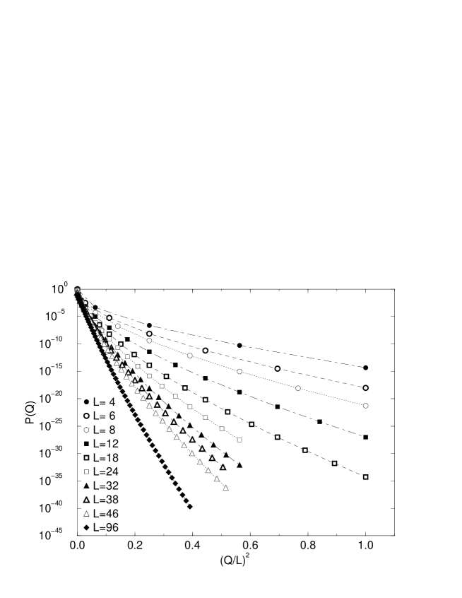
Fig. 1: Probability distribution of the topological charge for ${\rm CP}^{3}$FP with $\beta=3.0$ and various values of $L$. Only the results with $Q/L\leq 1$ are plotted. The size of error bars is such that they cannot be seen at this scale of plotting. The curves connecting the data points are included as a guide to the eye.

In Fig. 1 we plot the measured topological charge distribution $P(Q)$ with $\beta=3.0$ for various lattice sizes $L$. For convenience and to present data in a compact manner, we normalize the topological charge with the lattice size $L$. Even a rough inspection of the figure reveals that the data do not exhibit Gaussian behavior, which would be represented by straight lines with this method of plotting. In particular, the data for small lattice sizes exhibit a clear curvature, while they tend to straighten out to some extent as the lattice size increases. However, fits with a Gaussian form turn out to be extremely poor for all the cases.

In Fig. 2 we compare the charge distribution obtained with the two weak couplings $\beta=3.0$ and 3.4 for a scaling check of $P(Q)$. For such a comparison to be possible, we have now to normalize the charge with the physical lattice size $L/\xi$, for which we use measured values of the correlation length $\xi$. We find that the data at the two couplings exhibit the same behavior and lie roughly on the same line. The remaining differences are most visible towards larger values of the topological charge. This may be explained by the following two reasons. One is that the physical lattice sizes can differ slightly. Values of $L/\xi$ are 1.687(6) (L=12), 3.37(1) (L=24), 4.50(2) (L=32) for $\beta=3.0$ and 1.68(2) (L=22), 3.36(4) (L=44), 4.43(6) (L=58) for $\beta=3.4$. The other is that $\xi$ is chosen from Table II for each $\beta$ . We take $\xi$ to be 7.114(27) for $\beta=3.0$ and 13.08(17) for $\beta=3.4$. If the measured values of $\xi$ were used for each $L$, one would expect at most a 10 $\%$ difference among the values of $\xi$ in this range of $L$, but the quality of the agreement of the values of $P(Q)$ in the figure does not change. In a strict sense, we are not able to obtain rigorous scaling behavior, but the quality of the agreement of the two different values of $\beta$ is still remarkably good compared to the other two models, ${\rm CP}^{1}$FP and ${\rm CP}^{3}$ST. This point is discussed in detail in the following section (see Fig. 11). For an argument of more rigorous scaling, we need to use measured $\xi$ for each $L$ and use $Q_{{\rm FP}}$ instead of $Q_{{\rm ST}}$, but here we think the results in Fig. 2 are sufficient for the present discussion.

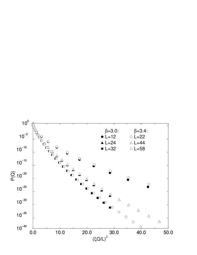
Fig. 2: Scaling test of the charge probability distribution for ${\rm CP}^{3}$FP at two values of the coupling and several volumes.

3.2.2 Correlation length

Simulations with the set method allowed us to determine the dependence of the correlation length on the topological charge. Correlation functions can be measured separately for different topological sectors, and correlation lengths $\xi(Q)$ can be extracted from their fall-off at large time separations. The results are shown in Fig. 3, where we plot correlation lengths as functions of the charge density. We normalize the charge density by the correlation length $\xi(\theta=0)$ obtained from simulations without a topological term discussed in Sec. 3.1.

In the left panel of Fig. 3, we plot the data obtained with $\beta=3.0$ and different lattice sizes. As expected, the data fall on a universal curve if plotted as functions of the topological charge density. We find a decrease of the correlation length with increasing topological charge density. The reason for this is that with an increasing number of topological objects within the same volume, the configuration has to become less ordered. At the point where the topological charge density $Q/(L/\xi(\theta=0))^{2}$ is equal to 1, the correlation length $\xi(Q)$ has dropped to less than half of its value at zero topological charge. In the right panel of Fig. 3 we compare representative data at two different values of the coupling constant. We see clear scaling behavior of $\xi(Q)/L$. For smaller values of $\xi(Q)$, on the other hand, we have observed violations of the scaling property. The curve for $\beta=3.0$ starts to deviate at $Q/(L/\xi(\theta=0))^{2}\approx 0.7$ where $\xi\approx 4$. This, in turn, indicates that even a use of the FP action is unable to suppress the lattice defects for $\xi\leq 4$, which is in agreement with similar previous observations. [8, 20]

From these scaling checks, we conclude that the observed behaviors of $P(Q)$ and $\xi(Q)$ for $\beta=3.0$ represent continuum properties and are not caused by lattice artifacts. These are compared with the results for ${\rm CP}^{1}$FP and ${\rm CP}^{3}$ST actions in the following section.

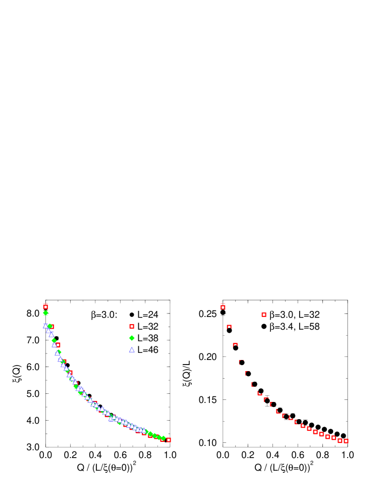
Fig. 3: Fixed charge sector correlation length as a function of the physical charge density for ${\rm CP}^{3}$FP. In the left panel we compare various lattice sizes at $\beta=3.0$ and in the right panel we show scaling between $\beta=3.0$ and 3.4.

3.3 Free energy density and expectation value of the topological charge

In Fig. 4 we show results for the free energy density obtained with Eq. (2.12) for $\beta=3.0$ and several lattice sizes $L$. Central values are indicated by solid lines, while the one-sigma error bands, determined with a jack-knife analysis, are represented by dashed lines. We obtain smooth curves, and no “flattening” is observed, as in some other works. [11, 18, 19] The only exception is the simulation with $L=96$ (not shown in the figure), where the calculation of $F(\theta)$ breaks down at $\theta\approx 1$, because the partition function turns out to be negative (while still consistent with zero within the error bars). Before this breakdown, the error bars become very large.

Fig. 4: Free energy density $F(\theta)$ for ${\rm CP}^{3}$FP for $\beta=3.0$ and several lattice sizes $L$.

Note that the physical free energy densities for the corresponding lattice sizes of $\beta=3.0$ and $\beta=3.4$ fall on the same curve, which is a consequence of the scaling of $P(Q)$ shown in Fig. 2. We observe a strong dependence of the free energy density on the lattice size. $F(\theta)$ increases with increasing $L$ and for $\theta<1$, already, nearly asymptotic values are obtained for our largest lattice sizes. This is, however, not yet the case for $\theta$ close to $\pi$. This has the consequence that curves become steeper as the volume increases. Does this mean that $F(\theta)$ develops a peak at $\theta=\pi$, which would be an indication of a phase transition?

To answer this question, we consider the expectation value of the topological charge obtained with Eq. (2.13). We show results obtained for $\beta=3.0$ in Fig. 5. As seen there, $\langle Q\rangle_{\theta}$ vanishes both for $\theta=0$ and $\pi$. In between these values, it has a peak, which we observe to move slowly away from $\theta=\pi/2$, obtained at small lattices, towards $\pi$. Figure 6 displays the volume dependence of $\theta_{\rm max}$, defined to be the position of the peak of $\langle Q\rangle_{\theta}$. This clearly shows how $\theta_{\rm max}$ moves away from $\pi/2$. It is, however, still far from $\pi$ even with our largest lattice, and it cannot be conclusively determined from our data where the infinite volume limit of $\theta_{\rm max}$ is.

Fig. 5: Expectation value of the topological charge $\langle Q\rangle_{\theta}$ for ${\rm CP}^{3}$FP with $\beta=3.0$ and several lattice sizes $L$. Results increase from $L=4$ (data points at the bottom) to $L=46$ (data points at the top).

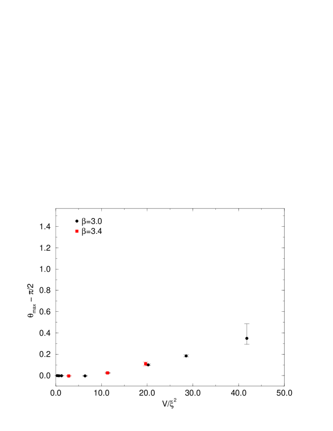
Fig. 6: Angle $\theta_{\rm max}$ of the maximal topological charge for ${\rm CP}^{3}$FP as a function of the physical lattice volume.

3.4 Effective power $\gamma_{\it eff}$ of $P(Q)$

We are now in a position to investigate the behavior of the charge distribution in more detail without having to be concerned about discretization effects. This is important for obtaining information about the underlying physics. Having observed that $P(Q)$ cannot be fit with a simple Gaussian, we turn to a closer examination of its local properties. To this end, we calculate the effective power $\gamma_{\it eff}=\gamma_{\it eff}(Q)$ defined by assuming that $P(Q)$ behaves at the three adjacent charges $Q$, $Q+1$ and $Q+2$ as the function

$$P_{\rm local}(Q)=A\exp(-BQ^{\gamma_{\it eff}}).$$ (3.2)

Since three values of the charge distribution are used as inputs and the function in Eq. (3.2) has three free parameters, the latter can be calculated algebraically without involving a fit. Trivially, the Gaussian distribution takes the value $\gamma_{\it eff}=2$, independent of $Q$.

Results for $\gamma_{\it eff}(Q)$ with $\beta=3.0$ are displayed in Fig. 7 as a function of the charge density or charge filling fraction $Q/V$ of the lattice. We plot the same data twice, first showing all results up to large filling fractions in the left panel, and then zooming in to the region of small filling fractions in the right panel, where data for small (4, 6 and 8) and large (96) lattice sizes are omitted for clearer visibility.

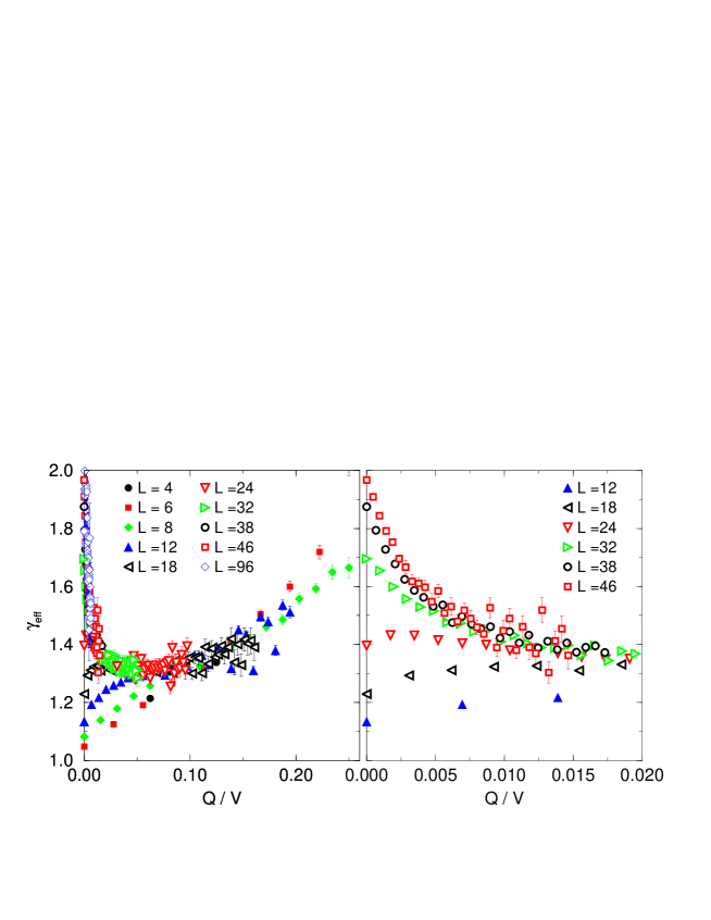
Fig. 7: Effective power of the probability distribution for ${\rm CP}^{3}$FP with $\beta=3.0$ and various lattice sizes. The left panel shows all results up to a charge filling fraction of $1/4$, while the right panel is an enlargement of the region with small filling fraction.

We observe that for almost all the combinations of lattice size $L$ and topological charge $Q$, the values of $\gamma_{\it eff}$ differ considerably from 2. This explains why we could not fit $P(Q)$ with a Gaussian. In fact, $P(Q)$ is not even well described locally by a Gaussian for most of the cases. We find, however, that the values of $\gamma_{\it eff}(Q)$ are bounded between the two limits 1 and 2. The values found at $Q=0$ depend on the lattice size. When the topological charge is increased, we find that results from different lattice sizes seem to approach a common value of $\gamma_{\it eff}\approx 1.3$. This common value is reached, at the latest, at a filling fraction of around $1/10$. An interesting point to observe is that the approach to this common value is from two different sides, depending on the lattice size. Data for $L=12$, for example, start with $\gamma_{\it eff}=1.13$ at $Q=0$ and increase with increasing charge. As an example of different behavior, data for $L=38$ start with $\gamma_{\it eff}=1.88$ at $Q=0$ and decrease with increasing charge. The lattice size at which increasing behavior changes to decreasing behavior is approximately $L=24$ (which corresponds to $L/\xi\approx 3.5$).

If we increase the topological charge to filling fractions larger than about $1/10$, the values of $\gamma_{\it eff}$ move away from 1.3 and increase in a universal manner. This can be easily understood to be an effect of approaching the limit of the maximal number of topological objects (instantons) that can be placed on a lattice. The probability of such densely packed lattice configurations is decreased, which, in turn, leads to an enhancement of $\gamma_{\it eff}$. This point will be investigated in section 5 by studying analytical models.

In Fig. 8 we compare the results for $\gamma_{\rm eff}$ at the two weak couplings, $\beta=3.0$ and 3.4. In order to make this comparison, we have to plot the data as a function of the physical charge density instead of the filling fraction. By doing this, the data at the two couplings collapse to a common line, showing scaling also for $\gamma_{\it eff}$. This finding also confirms the approach from different sides to the asymptotic value for different physical lattice sizes.

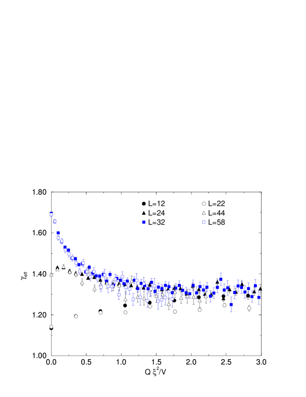
Fig. 8: Scaling test of $\gamma_{\it eff}$ for ${\rm CP}^{3}$FP with $\beta=3.0$ (solid symbols) and $\beta=3.4$ (open symbols).

Let us finally focus on the value of $\gamma_{\it eff}$ obtained at the origin, $Q=0$. As observed in Fig. 7, it takes values between 1 and 2 and exhibits strong dependence on the lattice size. This lattice size dependence is shown in Fig. 9. We clearly observe a crossover from values close to 1 for small lattices to values approaching 2 in the limit of large lattices. In this way, we recover a Gaussian charge distribution at weak coupling. It is realized, however, only in the limit of large volume and only near vanishing topological charge.

Fig. 9: Effective power $\gamma_{\it eff}$ at the origin as a function of the lattice size $L$ for ${\rm CP}^{3}$FP at $\beta=3.0$.

The effect observed at weak coupling is also observed for strong coupling, as shown in Fig. 10. Here we find $\gamma_{\it eff}$ to be around 2, in accordance with the observation of Gaussian behavior at strong coupling in Refs. [10] and [11]. However, if the filling fraction becomes large, we again see an increase of $\gamma_{\it eff}$, so that even values larger than 2 can be obtained.

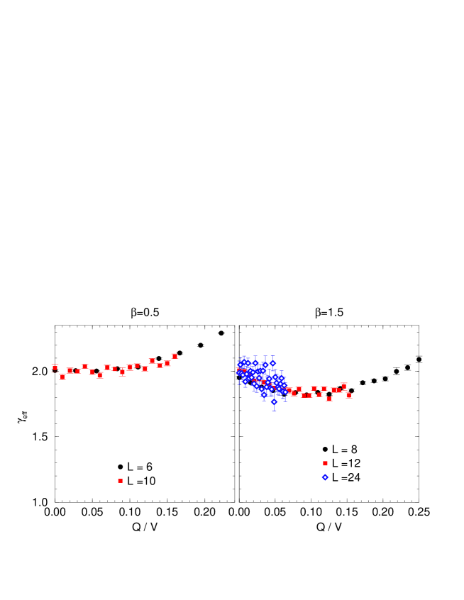
Fig. 10: $\gamma_{\it eff}$ for ${\rm CP}^{3}$FP at strong couplings.

It is interesting to note in connection to this behavior that numerical simulations in the strong coupling region, where a Gaussian distribution was observed in previous studies, [10, 11] are confined at the same time in a region of large volumes and in a region of small physical charge density. The reason for this is that for a strong coupling, the correlation length $\xi$ is small. The lattice size $L$, however, should not be chosen to be small, so that the lattice can contain more than just a few instantons. As a result, the ratio $L/\xi$ becomes large, which means that we are in a region of large physical volumes. Moreover, even though in the above-mentioned previous calculations the range of $Q$ was taken up to fairly large values, they still correspond to a small physical charge density $\xi^{2}Q/V$, because values of $L/\xi$ are large.

4 Numerical results for ${\rm CP}^{1}$FP and ${\rm CP}^{3}$ST

It is worthwhile to investigate whether scaling behavior is observed, and if not, to what extent it breaks down for other cases of the ${\rm CP}^{N-1}$ model. For comparison, we considered a model with ${\rm CP}^{1}$ FP action. As a parametrization of the ${\rm CP}^{1}$FP action, we used the parametrization listed in Table 4 of the original paper by Hasenfratz and Niedermayer, [5] in which 24 local coupling constants are employed. For updating configurations, we used the Metropolis algorithm. Typically, we performed one to several million sweeps per set, depending on the coupling constant $\beta$ and $L$. For the set method described in section 2, we always chose 4 bins for each set and the trial function to be Gaussian. The values of $\beta$ ranged from 0.7 to 1.1 and the lattice sizes from 12 to 62.

In order to study the scaling behavior, we compare the results for pairs of parameter doublets $(\beta,L)$, as done in the previous section, so that each one of the pair is chosen to have approximately the same physical volume, $(L/\xi(\theta=0))^{2}$. Figures 11 and 12 show $P(Q)$ and $F(\theta)$, respectively, for ($\beta$, $L$)=(0.87,22) and (1.02, 44), where $L/\xi(\theta=0)$ is measured to be 3.2. These data exhibit a large difference, in contrast to the ${\rm CP}^{3}$FP case depicted in Fig. 2, and the scaling is found to be clearly broken. In Fig. 13 we compare the correlation lengths $\xi/L$ as a function of the physical charge density $Q/(L/\xi(\theta=0))^{2}$. The two sets of data for $\xi/L$ also exhibit strong scaling violation, and large deviation($\approx 30\%$) is found for $Q/(L/\xi(\theta=0))^{2}\approx 0.7$. It is noted that this behavior is also seen for other choices of pairs with different values of $L/\xi(\theta=0)$, e.g., $(\beta,L)$ =(0.7, 12) and (0.9,30), with $L/\xi(\theta=0)$ being 3.6.

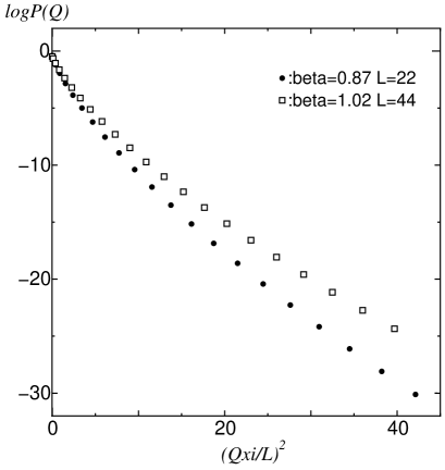
Fig. 11: Topological charge distribution $\log P(Q)$ vs $(Q\xi(\theta=0)/L)^{2}$ for ${\rm CP}^{1}$FP. ($\beta$, $L$) = (0.87,22) corresponds to the solid dots and (1.02,44) to the open boxes.

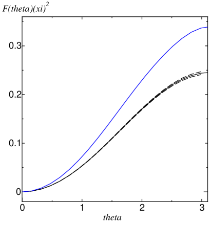
Fig. 12: Physical free energy density $F(\theta)\xi^{2}$ for ${\rm CP}^{1}$FP. The upper curve corresponds to ($\beta$, $L$) = (0.87,22) and the lower to (1.02,44).

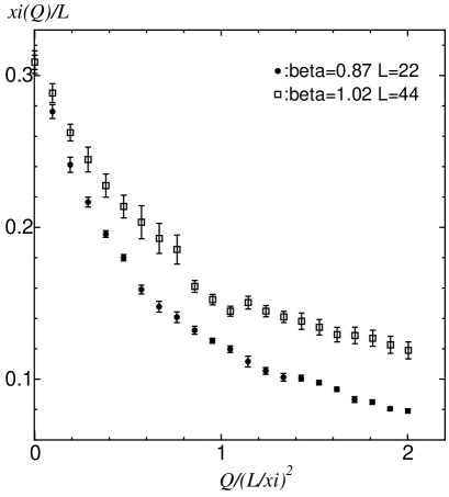
Fig. 13: The correlation length $\xi/L$ as a function of $Q/(L/\xi(\theta=0))^{2}$. ($\beta$, $L$) = (0.87,22) corresponds to the solid dots and (1.02,44) to the open boxes.

We have found for the ${\rm CP}^{1}$ model that scaling is strongly violated, although the FP action is used. This is expected, since it is well known that dislocations do harm seriously in the ${\rm CP}^{1}$ model. In our calculations, we have used only the FP action, and the additional use of a FP charge might be expected to produce better results. However, we suspect that even if we had used the FP charge, the scaling nature would not have been improved. This comes from the observation that even after the dislocations are eliminated by a combined use of the FP charge and the FP action, the scaling behavior of the lattice topological susceptibility $\chi_{t}$ is strongly violated. [6, 7]

We have also calculated the ${\rm CP}^{3}$ standard action for different choices of $\beta$ and $L$. We varied lattice sizes from 18 to 54 and $\beta$ from 1.8 to 2.3 and looked for pairs of doublets $(\beta,L)$ such that $L/\xi$ for each pair is approximately the same. Values of $L/\xi$ were chosen to be from about 2.7 up to 4.2, which are similar to the values used for CP¹FP and CP³FP. For updating configurations, we used the Metropolis algorithm, and the number of sweeps used for each set was approximately same as for CP¹FP. Use of the standard action for the ${\rm CP}^{3}$ model exhibits strong violation, similar to the case ${\rm CP}^{1}$FP, for $P(Q)$ and $F(\theta)$, as well as the correlation length $\xi/L$. This is easily understood, since the standard action is very poor in representing continuum physics. The behavior of $\xi/L$ exhibits somewhat small deviation compared to that for CP¹FP.

5 Debye-Hückel approximation

In Refs. [10] and [11] it has been shown that a first-order phase transition exists at $\theta=\pi$ when the topological charge distribution $P(Q)$ is Gaussian, and its volume dependence is given by $P(Q)\sim\exp[-\alpha Q^{2}/V]$, where $\alpha$ is a constant that depends on the coupling constant $\beta$. Such a Gaussian charge distribution has been found in the region of very strong coupling. As $\beta$ becomes larger for some fixed volume, $P(Q)$ has been observed to deviate from the Gaussian form, and thus the first-order phase transition gradually disappears. We note that $P(Q)$ for a system that consists of instantons and anti-instantons obeying the Poisson distribution also behaves like a Gaussian for values of the parameter corresponding to the strong coupling region. Therefore, we expect instantons and anti-instantons in such a system to behave like a dilute gas in the strong coupling region. It is thus of interest to determine the nature of the dynamics of instantons displayed by a system for which $P(Q)$ is not Gaussian. In order to investigate this issue, we use the Debye-Hückel model, [12] which is based on an instanton quark picture, [13] and in which correlations between particles (instanton quarks) are weak.

5.1 Instanton quark picture and Debye-Hückel model

In this subsection we explain the concept of the instanton quark picture and the Debye-Hückel model (D-H model). In order for this paper to be self-contained, we also give a summarized overview of the results obtained in previous works. [12, 13] In Ref. [13], Fateev, Frolov and Schwarz analyzed Euclidean Green’s functions and the partition function to investigate how instantons affect the dynamics of the CP^N-1 model. The partition function of this model in the continuum is defined by

$$Z=\int{\cal D}z{\cal D}\overline{z}\prod_{x}\delta(\sum_{\alpha=1}^{N}|z_{\alpha}(x)|^{2}-1)e^{-S},$$ (5.1)

and the action is defined by

$$S=\beta\int d^{2}x\sum_{\alpha=1}^{N}\{|\partial_{\mu}z_{\alpha}(x)|^{2}+(\overline{z}_{\alpha}(x)\partial_{\mu}z_{\alpha}(x))^{2}\},$$ (5.2)

where $\overline{z}_{\alpha}$ denotes the complex conjugate of $z_{\alpha}$. The $(N-1)$-dimensional complex projective space is defined by introducing a field as

$${\it w}_{\alpha}(\zeta)=z_{\alpha}(\zeta){\hbox{$\left/\vbox to0.0pt{}\right.\n@space$}}z_{N}(\zeta) ;\;\alpha=1,2,\cdots,N-1\; ,\mbox{where }z_{N}(\zeta)\neq 0,$$ (5.3)

in the complex plane $\zeta=x+iy$. As a next step, the action is rewritten in the form

$$S=\beta\int d^{2}x\frac{1}{1+\rho^{2}}\Bigl{[}\sum_{\alpha}|\partial_{\mu}{\it w}_{\alpha}|^{2}-\frac{\sum_{\alpha}\overline{{\it w}}_{\alpha}\partial_{\mu}{\it w}_{\alpha}\sum_{\gamma}{\it w}_{\gamma}\partial_{\mu}\overline{{\it w}}_{\gamma}}{1+\rho^{2}}\Bigr{]},$$ (5.4)

where $\rho^{2}=\sum_{\alpha=1}^{N-1}|{\it w}_{\alpha}|^{2}$ and $d^{2}x=\frac{1}{2}d\zeta d\overline{\zeta}$. A general $q$-instanton solution is given by

$$z_{\alpha}(\zeta)=c_{\alpha}\prod_{i=1}^{q}(\zeta-a_{\alpha}^{i}),$$ (5.5)

where $c_{\alpha}$ and $a_{\alpha}^{i}$ are complex parameters. The superscript $i\>(\,i=1,2,\cdots,q)$ labels instantons, and the subscript $\alpha\>(\,\alpha=1,2,\cdots,N)$ indicates the degrees of freedom of the field $z_{\alpha}$. The authors of Ref. [13] investigated how the system behaves when the field fluctuates around the $q$-instanton solution [21, 22] and showed that the partition function takes the form

$$Z=\sum_{q}W^{q}(q!)^{-N}\int\prod_{\alpha=1}^{N}\prod_{i=1}^{q}d^{2}c_{\alpha}d^{2}a_{\alpha}^{i}\exp\bigl{\{}-{\cal H}_{q}(a,c)/T\bigr{\}}\delta\bigl{(}\sum_{\alpha=1}^{N}|c_{\alpha}|^{2}-1\bigr{)},$$ (5.6)

where $W$ is a constant that depends on the topological charge, and $T=1$. ${\cal H}_{q}$ in Eq. (5.6) is given by

$${\cal H}_{q}(a,c)=\frac{N}{4\pi}\int d^{2}x\Bigl{[}\log\rho\partial^{2}\log\rho-\log\bigl{(}\prod_{\alpha}|c_{\alpha}|^{2q}\prod_{i>j}|a_{\alpha}^{i}-a_{\beta}^{j}|^{2})\Bigr{]}.$$ (5.7)

Equation (5.6) can be interpreted as the partition function of a system of two-dimensional classical particles with interaction energy given by Eq. (5.7) in the grand canonical ensemble. The classical particles are at positions $a_{\alpha}^{i}$ and interact with each other. Note that $T$ plays the role of a temperature.

In the particular case $N=2$, i.e. for the ${\cal O}(3)$ non-linear sigma model, the grand partition function is given by

$$Z^{\prime} = \sum_{q}W^{q}(q!)^{-2}\int\prod_{i}d^{2}a_{1}^{i}d^{2}a_{2}^{i}\exp\bigl{\{}-{\cal H}^{\prime}_{q}(a)/T\bigr{\}},$$ (5.8)

$${\cal H}^{\prime}_{q}(a) = -\sum_{i<j}^{q}\log|a_{1}^{i}-a_{1}^{j}|^{2}-\sum_{i<j}^{q}\log|a_{2}^{i}-a_{2}^{j}|^{2}+\sum_{i,j}\log|a_{1}^{i}-a_{2}^{j}|^{2}.$$ (5.9)

We see that in the Hamiltonian (5.9), a particle possesses a “charge”$(\alpha=1,2)$ and that particles of equal charge interact repulsively, while those of opposite charge interact attractively. Thus we can interpret this model as a two-dimensional classical Coulomb system that consists of $2q$ particles with positive and negative charges. Furthermore, if the locations $\{a_{\alpha}^{i};i=1,2,\cdots,q,\alpha=1,2\}$ satisfy the conditions $|a_{1}^{i}-a_{2}^{i}|\ll|a_{1}^{i}-a_{1}^{j}|,|a_{2}^{i}-a_{2}^{j}|(i\neq j)$, we can regard $\frac{1}{2}(a_{1}^{i}+a_{2}^{i})$ as the position and $\frac{1}{2}|a_{1}^{i}-a_{2}^{i}|$ as the size of the $i$-th instanton. Due to the interaction (5.9), a pair of particles with opposite charges tends to make up an instanton with neutral charge. For this reason, the particles are called “instanton quarks”. [13]

In the case of a $\overline{q}$-anti-instanton configuration, the solution is given by

$$z_{\alpha}(\zeta)=\overline{c}_{\alpha}\prod_{i=1}^{\overline{q}}(\overline{\zeta}-\overline{b}_{\alpha}^{i}),\;\alpha=1,2,$$

and the partition function has the same form as in Eq. (5.8) but with the variables $a_{\alpha}^{i}$ replaced by $b_{\alpha}^{i}$. In analogy with the ${\cal O}(3)$ non-linear sigma model, the CP^N-1 model can be interpreted as a classical system that consists of instanton quarks with “multicolors” $(\alpha=1,2,\cdots,N)$ such that instanton quarks with the same color interact repulsively and those with different colors interact attractively.

Recently Diakonov and Maul [12] investigated the effects of instantons and anti-instantons for the CP^N-1 model by using the instanton quark picture. They proposed a configuration with $N_{+}$ instantons and $N_{-}$ anti-instantons by assuming a product ansatz of the form [23]

$$z_{\alpha}(\zeta)=\prod_{i=1}^{N_{+}}(\zeta-a_{\alpha}^{i})\prod_{j=1}^{N_{-}}(\overline{\zeta}-\overline{b}_{\alpha}^{j}),$$

where $\alpha=1,2,\cdots,N$. Since Eq. (5.7) cannot be analytically solved for $N>2$, they simplified the multi-body interaction into an interaction of the two-body type. Furthermore, they applied the Debye-Hückel approximation to this model; i.e., they assumed that the correlations between instanton quarks are very weak and individual quarks interact with a mean field. The partition function turns out to be

$$Z(\theta)=\sum_{N_{+},N_{-}}Z(N_{+},N_{-})\exp\{i\theta(N_{+}-N_{-})\},$$ (5.10)

where the partition function $Z(N_{+},N_{-})$ is given by

$$Z(N_{+},N_{-}) = \exp\Biggl{[}-\frac{N^{2}V_{d}}{4(N-1)}\beta\biggl{\{}\frac{\tilde{n}_{+}+\tilde{n}_{-}}{2}\Bigl{(}\log\frac{\tilde{\mathchar 28931\relax}^{2}}{4\pi\beta\sqrt{\tilde{n}_{+}\tilde{n}_{-}(1-\beta^{\prime 2})}}+1\Bigr{)}$$

$$-\frac{1}{4}\sqrt{(\tilde{n}_{+}-\tilde{n}_{-})^{2}+4\tilde{n}_{+}\tilde{n}_{-}\beta^{\prime 2}}\log\frac{\kappa_{+}}{\kappa_{-}}\biggr{\}}\biggr{]}\frac{(V_{d}\mathchar 28931\relax^{2})^{N(N_{+}+N_{-})}}{(N_{+}!)^{N}(N_{-}!)^{N}}.$$

Here

$$\beta = 1/T$$

$$\tilde{n}_{\pm} = \frac{N}{N-1}\frac{N_{\pm}}{V_{d}}$$

$$\kappa_{\pm} = 2\pi\beta{\hbox{$\left[\vbox to0.0pt{}\right.\n@space$}}(\tilde{n}_{+}+\tilde{n}_{-})\pm\sqrt{(\tilde{n}_{+}-\tilde{n}_{-})^{2}+4\tilde{n}_{+}\tilde{n}_{-}\beta^{\prime 2}}\bigr{]}$$

$$\tilde{\mathchar 28931\relax} = 2\mathchar 28931\relax e^{\gamma_{E}}.$$

In the above, $\beta^{\prime}$ is a coupling constant between instanton quarks and anti-instanton quarks introduced by the ansatz represented by Eq. (5.1), and $V_{d}(\equiv L_{d}^{2})$ is the volume of the system in the continuum. $\mathchar 28931\relax$ is a parameter like $\mathchar 28931\relax_{QCD}$, and $\gamma_{E}$ is the Euler number. Note that $T$ plays the role of a temperature ( here $T=1$).

We calculate $P(Q)$ from Eq. (5.1) as

$$Z(\theta) =\sum_{N_{+},N_{-}}Z(N_{+},N_{-})\exp\{i\theta(N_{+}-N_{-})\}$$ (5.12)

$$=\sum_{Q}\sum_{N_{+},N_{-}}\delta_{N_{+}-N_{-},Q}Z(N_{+},N_{-})\exp\{i\theta(N_{+}-N_{-})\}$$

$$\equiv\sum_{Q}\exp\{i\theta Q\}P(Q),$$

where

$$P(Q)\equiv\sum_{N_{+},N_{-}}\delta_{N_{+}-N_{-},Q}Z(N_{+},N_{-}).$$

We carefully consider the behavior of $P(Q)$ in the next subsection.

5.2 Analysis of P(Q) in terms of the instanton picture based on instanton quarks

We now discuss the topological charge distribution $P(Q)$ in terms of instantons (anti-instantons). Before referring to $P(Q)$, let us first consider the behavior of $Z(N_{+},N_{-})$. In Fig. 14 we give a two-dimensional plot of $Z(N_{+},N_{-})$ obtained from Eq. (5.1) for $L_{d}=4$, $\beta=1.0$ and $\beta^{\prime}=0.0$. These values of the parameters were chosen to be the same as those in Ref. [12]. From this point, we set $\mathchar 28931\relax$ to unity. [12]

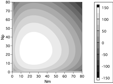
Fig. 14: Two-dimensional plot of the partition function $\log Z(N_{+},N_{-})$ for N=4, $L_{d}=4$, $\beta=1.0$ and $\beta^{\prime}=0.0$. Only results with $1\leq N_{p},N_{m}\leq 80$ are plotted. Here $N_{p}$ and $N_{m}$ are the number of instantons and anti-instantons, respectively.

Figure 14 displays typical behavior of $Z(N_{+},N_{-})$. This function is symmetric under interchange of $N_{+}$ and $N_{-}$ and has a maximum at some non-zero value of $N_{+}(=N_{-})$. The region around the maximum gives a dominant contribution to the charge distribution $P(Q)$ at $Q=0$. It is interesting to see that a fairly large number of instantons $(N_{+}=N_{-}\approx 30)$ contribute to $P(0)$.

Fig. 15: The logarithm of $Z(N_{+},N_{-})$ for the case Q=0 with $\beta=1.0$ and $L_{d}=4$. The results for $\beta^{\prime}=0.0$ are represented by solid dots and the results for $\beta^{\prime}=0.5$ by crosses.

Fig. 16: The logarithm of $Z(N_{+},N_{-})$ in the case Q=0 with $L_{d}=4$ and $\beta^{\prime}=0.0$. $\beta$ is chosen as 0.1($\bullet$), 0.5($+$) and 1.0($\times$).

In Fig. 16 we compare $Z(N_{+},N_{-})$ for two different values of $\beta^{\prime}$ ($\beta^{\prime}=0.5$ and $\beta^{\prime}=0.0$) in the case $Q=0$ $(N_{+}=N_{-})$. We find that $Z(N_{+},N_{-})$ has only weak $\beta^{\prime}$ dependence. In fact, this is true for other choices of the parameters as well. This result shows that the correlations between instanton quarks and anti-instanton quarks can be ignored. [12] For this reason, we set $\beta^{\prime}=0$. Figure 16 shows how $Z(N_{+},N_{-})$ depends on $\beta$ for a fixed volume. We see that as $\beta$ becomes larger, the position of the maximum of $Z(N_{+},N_{-})$ shifts to the right and configurations with larger numbers of instantons and anti-instantons are generated. Note that $\beta=1.0$ corresponds to a physical system. For fixed $\beta$, on the other hand, the peak of $Z(N_{+},N_{-})$ shifts upward and to the right with increasing volume. This is intuitively understandable.

We are now in a position to study $P(Q)$.

Fig. 17: The logarithm of $P(Q)$ as a function of $Q^{2}$ in the Debye-Hückel approximation for $\beta=1.0$, $\beta^{\prime}=0.0$ and $L_{d}=4$.

Fig. 18: $\gamma_{\it eff}^{(D)}$ obtained from $P(Q)$ for $\beta=1.0$, $\beta^{\prime}=0.0$ and $L_{d}=4$.

In Fig. 18 we plot $P(Q)$ obtained from $Z(N_{+},N_{-})$ for $\beta=1.0$ and $L_{d}=4$. At first sight, $P(Q)$ looks like a Gaussian. In order to investigate the behavior of $P(Q)$ in more detail, we calculate the effective power $\gamma_{\it eff}$ introduced in subsection 3.4. We recall that in Monte-Carlo simulations, $\gamma_{\it eff}$ is nearly equal to 2.0 at $Q/V=0$ and decreases slowly with increasing charge for large volumes, while for small volumes, $\gamma_{\it eff}$ is near unity at $Q/V=0$ and increases rapidly with increasing charge. It is interesting to investigate the cause of this difference and whether it can be accounted for by the D-H model. In Fig. 18 we display $\gamma_{\it eff}^{(D)}$ as a function of the physical charge density $Q/V_{d}$, where $\gamma_{\it eff}^{(D)}$ is obtained in the D-H approximation. Obviously $\gamma_{\it eff}^{(D)}$ is different from 2.0 (Gaussian). Even if we take $\beta^{\prime}\neq 0$, the results do not change significantly. Compared to Fig. 7, the D-H approximation is found to reproduce the behavior of $\gamma_{\it eff}$ for large volumes.

Let us now turn to small volumes, for which we believe that finite size effects are relevant for $P(Q)$ on a lattice. Since instantons with a size smaller than the lattice spacing fall through the lattice, the number of instantons is bounded from above ($\equiv N_{max}^{(lat)}$) in finite volumes. Contrastingly, the D-H model is defined in the continuum, and for it, an infinite number of instantons can be placed in finite volume. In order to reproduce the lattice results with this model, it is necessary to restrict the upper limit ($\equiv N_{max}$) to a finite value in the summation $\sum_{N_{+},N_{-}}Z(N_{+},N_{-})$ in Eq. (5.1). Let us assume that $N_{max}$ mimics $N_{max}^{(lat)}$.

Fig. 19: Same as in Fig. 18, but with an upper limit $N_{max}$ in the summation $\sum_{N_{+},N_{-}}Z(N_{+},N_{-})$. $N_{max}$ is taken to be 25($\bullet$), 50($\times$) and 75($+$).

In Fig. 19 we display the results for $\beta=1.0$ and $L_{d}=4$ with three different choices of $N_{max}$. For large $N_{max}$ ($>40$), starting at $Q=0$, $\gamma_{\it eff}^{(D)}$ gradually decreases from $2.0$ and starts to diverge at some non-zero value of $Q/V_{d}$. For smaller values of $N_{max}(=25)$, $\gamma_{\it eff}^{(D)}$ is close to unity at $Q=0$ and increases rapidly as a function of $Q$. At some small value of the filling fraction, $\gamma_{\it eff}^{(D)}$ overshoots 2.0. The behavior seen in Fig. 19 is quite similar to that seen in Fig. 7. It is noted that $\gamma_{\it eff}^{(D)}$ at $Q/V_{d}=0$ gradually shifts up from 1.0 up to 2.0 if we increase $N_{max}$ for small values, in accordance with the behavior seen in Fig. 9.

We find by varying $N_{max}$ and by taking various values of $\beta$ and $L$ that when $N_{max}$ is chosen to be approximately equal to or less than the location of the peak of the distribution $Z(N_{+},N_{-})$ (see Fig. 14), $\gamma_{\it eff}^{(D)}$ at $Q=0$ starts at a value nearly equal to 1, and when $N_{max}$ is larger than the location of the peak, $\gamma_{\it eff}^{(D)}$ starts at 2. For the latter case, $\gamma_{\it eff}^{(D)}$ slowly decreases as a function of $Q/V_{d}$, and diverges at some value of $Q/V_{d}$. As $N_{max}$ becomes even larger, $\gamma_{\it eff}^{(D)}$ begins to diverge at a larger density $Q/V_{d}$. These observations allow us to conclude that the behavior of $P(Q)$ found in Monte Carlo simulations reflects the dynamics of weakly correlated instanton quarks.

5.3 Analysis of $P(Q)$ in terms of the Poisson distribution

Before ending this section, we study $\gamma_{\it eff}$ obtained from a system that consists of instantons and anti-instantons obeying the Poisson distribution. This is equivalent to a dilute gas system (DGA) of instantons and anti-instantons for which $P(Q)$ is given by

$$P(Q)=\sum_{N_{+},N_{-}}\frac{1}{2^{N_{+}+N_{-}}}\frac{(N_{+}+N_{-})!}{N_{+}!N_{-}!}P_{N_{+}+N_{-}}\delta_{N_{+}-N_{-},Q},$$

$$P_{n}\equiv\frac{\lambda^{n}}{n!}e^{-\lambda},$$

where $\lambda/2$ is the average number of instantons (anti-instantons).

Equation (5.3) leads in the limit $\lambda\to\infty$ to

$$P(Q)\sim\exp\bigl{\{}-\frac{1}{2\lambda}Q^{2}\bigr{\}}.$$ (5.13)

With the identification $\lambda=\frac{V}{2\alpha}$, Eq. (5.13) can be regarded as the distribution in the strong coupling region of MC simulations, where $\alpha$ is a constant that depends on $\beta$ appearing in $P(Q)\sim\exp[-\frac{\alpha}{V}Q^{2}]$ in such a manner that $\alpha\to 0$ as $\beta\to 0$.

Let us study how $\gamma_{\it eff}$ behaves for $\lambda<\infty$.

Fig. 20: $\gamma_{\it eff}^{(P)}$ for $\lambda=40$, where $\lambda$ is considered to be proportional to $V_{d}$.

Figure 20 displays $\gamma_{\it eff}(\equiv\gamma_{\it eff}^{(P)})$ as a function of $Q/\lambda$ for $\lambda=40$. We find that the behavior of $\gamma_{\it eff}^{(P)}$ is very similar to that of $\gamma_{\it eff}^{(D)}$ for various values of $N_{max}$, where $N_{max}$ is the upper limit of the summation in Eq. (5.3). Recalling that in the D-H model, correlations between instanton quarks are weak, while in the DGA there are no correlations between instantons, we can conclude that the D-H model also has little correlation between instantons.

6 Conclusions and discussion

• We have studied ${\rm CP}^{N-1}$ models with a topological term. In order to obtain a description of continuum physics, we have employed an FP action and investigated scaling properties of quantities such as $P(Q)$, $F(\theta)$ and the correlation length $\xi(Q)/L$. For ${\rm CP}^{3}$FP we have observed good scaling behavior, while for ${\rm CP}^{1}$FP and ${\rm CP}^{3}$ST we have found strong violations of scaling.

• We have investigated the effective power $\gamma_{\it eff}$ of $P(Q)$ for CP³FP. At a fixed value of $\beta$, $\gamma_{\it eff}$ increases from 1.0 for small lattices as $Q$ increases, while $\gamma_{\it eff}$ decreases from 2.0 for large $L$. The values of $\gamma_{\it eff}$ for both large and small lattices reach a common line at some small value of the filling fraction. When finite size effects become significant, the value of $\gamma_{\it eff}$ starts increasing beyond 2.0.

• We have studied the behavior of $\gamma_{\it eff}$ for the analytical models, the Debye-Hückel approximation to an instanton quark gas of the CP^N-1 model, and the Poisson distribution of an instanton gas. We have found that in these cases, $\gamma_{\it eff}$ exhibits the same behavior as that obtained in Monte Carlo simulations. Finite size effects, which emerge by packing instantons into a finite volume, show up as an increase beyond 2.0 of $\gamma_{\it eff}$. These observations allow us to conclude that $P(Q)$ obtained in MC simulations describes the dynamics of very weakly correlated instantons.

• Gaussian behavior of $P(Q)$ seems to be realized when volumes are large and the physical charge density is small. In the strong coupling region, these conditions are easily satisfied, because correlation lengths are very short in this region. As a consequence, there exists a first-order phase transition at $\theta=\pi$. In the weak coupling region, on the other hand, $\gamma_{\it eff}$ tends to be 2.0 only at vanishing topological charge when the volume increases. The expectation value $\langle Q\rangle_{\theta}$ develops a peak, and there is the tendency that the peak moves away from $\pi/2$ towards $\pi$ as the volume increases. However, we could not obtain conclusive results about existence of a phase transition in the infinite volume limit, because the above conditions are difficult to satisfy.

• When the volume is small, the value of $\gamma_{\it eff}$ increases from 1.0 as a function of the charge in all the cases we have investigated, not only for simulations but also for analytical models. It is an interesting question why $\gamma_{\it eff}$ is always bounded from below by 1.0. We think that perhaps this would be associated with some fundamental property of probability theory.

• Although the analytical models can explain the behavior of $\gamma_{\it eff}$ qualitatively well, $\gamma_{\it eff}$ for small volumes increases more rapidly than in MC simulations. This behavior might be due to the sharp cut-off ($N_{max}$) used in the summation in Eqs. (5.1) and  (5.3). We have tentatively smeared the cut-off by introducing a Gaussian function. As a result, we have observed that the increase of $\gamma_{\it eff}$ becomes somewhat less rapid, and it tends to follow the common line before diverging. However, in order to draw a definite conclusion, a more systematic study is needed.

• The fate of the first-order phase transition at $\theta=\pi$ in the strong coupling region is a relevant issue. As discussed in subsection 3.3, calculations of the free energy and the expectation value $\langle Q\rangle_{\theta}$ have huge errors already at $L=96$, and thus we cannot address this issue. To increase lattice size while keeping errors reasonably small requires an exponentially increasing number of sweeps. We may need some novel algorithm to overcome this problem.