The Weakly Coupled Gross-Neveu
Model with Wilson Fermions
R. Kenna and J.C. Sexton,
School of Mathematics, Trinity College Dublin, Ireland

March 2001

The nature of the phase transition in the lattice Gross-Neveu model with Wilson fermions is investigated using a new analytical technique. This involves a new type of weak coupling expansion which focuses on the partition function zeroes of the model. Its application to the single flavour Gross-Neveu model yields a phase diagram whose structure is consistent with that predicted from a saddle point approach. The existence of an Aoki phase is confirmed and its width in the weakly coupled region is determined. Parity, rather than chiral symmetry breaking naturally emerges as the driving mechanism for the phase transition.

1 Introduction

In continuum QCD, the conventional explanation for the smallness of the mass of pseudoscalar $\pi$ mesons is the following: QCD with $N_{f}$ massless quark flavours has a global chiral $U(N_{f})\times U(N_{f})$ symmetry, which, spontaneously broken, reduces to $U(N_{f})$ and yields $N_{f}^{2}$ Goldstone bosons. Explicit breaking of the original chiral symmetry by a small quark mass renders these $N_{f}^{2}$ Goldstone bosons massive with correspondingly small mass. To accord with nature, one of these Goldstone bosons (the $\eta$-particle in the case $N_{f}=2$) has to acquire an an additional mass. To explain this was known as the $U(1)$ problem in the continuum. Its resolution there comes from the axial anomaly, whereby the axial symmetry corresponding to the $U(1)$ subgroup of $U(N_{f})$ is explicitly broken by a quantum effect, reducing the number of Goldstone bosons to $N_{f}^{2}-1$.

Naive lattice regularization of such a fermionic theory is hindered by the doubling problem, namely that a return to the continuum manifests too many fermionic degrees of freedom. This doubling problem is resolved by the usage of Wilson fermions. However the extra Wilson term that removes the fermion doublers breaks chiral symmetry explicitly. This effect can be traced back to the existence of the axial anomaly in the continuum. For this reason the staggered format has often been the favoured one for the study of models with chiral symmetry breaking [1].

The Wilson action for free fermions in terms of dimensionless fermionic fields $\psi(n)$ defined at the sites $n$ of a $d$-dimensional lattice is

$$S_{F}^{(0)}[\bar{\psi},\psi]=\frac{1}{2\kappa}\sum_{n}{\bar{\psi}(n)\psi(n)}-\frac{1}{2}\sum_{n,\mu}{\left[\bar{\psi}(n)(r-\gamma_{\mu})\psi(n+\mu)+\bar{\psi}(n+\mu)(r+\gamma_{\mu})\psi(n)\right]}\quad,$$ (1.1)

where

$$1/2\kappa=\hat{M}_{0}+dr\quad.$$ (1.2)

Here, $\kappa$ is the hopping parameter, $r$ is the Wilson parameter, $a$ is the lattice spacing and $\hat{M}_{0}$ is a dimensionless fermion bare mass parameter. We use $d=2$ and $r=1$ throughout. This free fermion model is the weak coupling limit of an interactive theory in which a bare parameter $g$ measures the coupling of the free theory to some interaction. Even if $\hat{M}_{0}=0$, now, the Wilson term contributes to the hopping parameter and there is no obvious chiral symmetry. The question arises - what is the status of the chiral phase transition and the $U(1)$ problem on the lattice?

Despite the lack of an obvious chiral symmetry, there exists a host of numerical and analytical evidence for the existence of massless pions in the lattice formulation of QCD. These are believed to exist on a critical line $\kappa_{c}(g)$. In the literature, there are two explanations for the existence of the critical line and the masslessness of the lattice pions.

The first of these was sometimes referred to as the conventional explanation [2]. Although there is no obvious chiral symmetry at non-zero $r$, the conventional explanation suggests that tuning $\kappa$ effects its recovery in some unknown way. Now, with chiral symmetry recovered at $\kappa_{c}(g)$, the same arguments as in the continuum may be applied.

The second explanation was first forwarded in 1984 by Aoki [3]. Here it is accepted that since there is no chiral symmetry in the lattice formulation of QCD, its spontaneous breaking cannot be responsible for the masslessness of pions. Instead there is an Ising-like second order parity breaking phase transition. In the single flavour case the order parameter for parity symmetry is $\bar{\psi}i\gamma_{5}\psi$, the operator corresponding to the single $\pi$ meson. The parity symmetric phase is where $\langle\pi\rangle=\langle\bar{\psi}i\gamma_{5}\psi\rangle=0$. there is also a phase with long range order where $\langle\pi\rangle\neq 0$. At the transition between these phases, a correlation length $\xi$ diverges. This correlation length is identified as the inverse of the pion mass, which, hence, becomes zero on the phase boundary. Thus the pion is not a Goldstone boson in the Wilson lattice formulation. Aoki also recovered the current algebra relation between pion and quark mass ($m_{\pi}^{2}\sim m_{q}\sim(\kappa-\kappa_{c})$) by considering the effective meson theory as a scalar field theory in four dimensions with mean field like critical behaviour. In the multiflavour case the parity symmetry breaking is accompanied by a flavour symmetry breaking and, with it, Goldstone bosons in the form of the charged pions. The $\eta$ remains massive according to Aoki’s analysis, and the $U(1)$ problem in the lattice successfully resolved [3, 4].

Two main features distinguish Aoki’s QCD phase diagram from the conventional one. Firstly, the existence of the phase transition in Aoki’s scenario is due to parity symmetry breaking as opposed to chiral symmetry breaking in the conventional picture. The order parameter is $\langle\bar{\psi}i\gamma_{5}\psi\rangle$ rather than $\langle\bar{\psi}\psi\rangle$ [4]. Secondly, instead of a single critical line extending from the strongly coupled limit $g=\infty$ to $\kappa=1/2d$ in the weakly coupled limit $g=0$, Aoki’s picture involves the existence of two such lines and (in QCD) five critical points linked by four cusps in the weakly coupled zone.

Aoki’s QCD phase diagram is based on infinite-volume analyses in the limits of strong and weak coupling and on an analogy to the Gross-Neveu model, which, except for confinement, has features similar to QCD. One of these features is asymptotic freedom, so that in the Gross-Neveu model, as in QCD, the continuum limit is taken in the weakly coupled regime. Aoki’s scenario in the Gross-Neveu model again involves two critical lines spanning the full coupling range, with three critical points at zero coupling, linked by two cusps. This picture is based on saddle point methods [3]. There exists substantial evidence in support of this scenario in the strongly coupled regime [3, 4, 5, 6, 7, 8, 9, 10, 11, 12, 13]. In the weakly coupled regime, however, the evidence has been clear cut [14, 15] and this is the region where our attention is focused. Recently, also, Creutz [16] has posed a question as to the size of the Aoki phase. This question is whether the Aoki phase is “squeezed out” between the arms of the cusps at non-zero coupling or whether it only vanishes in the weak coupling limit [11, 12].

This sets the twofold motivation for this paper. Firstly, a new type of weak coupling expansion is developed [13]. From it, the partition function zeroes of Wilson fermionic models can be extracted in a natural way. This weak coupling technique is then applied to the Gross-Neveu model, where the existence of an Aoki phase was first suggested [3]. We confine our attention to the single flavour Gross-Neveu model and variants thereof. We also address the question of the “squeezing out” of the Aoki phase at weak coupling. This multiplicative approach to the single flavour Gross-Neveu model, shows that the width of the central Aoki cusp is ${\cal{O}}({g}^{2})$ while the Aoki phase has not yet emerged at this order from the left and right extremes. Furthermore, that parity symmetry breaking is the phase transition mechanism emerges in a very transparent way.

2 The Gross-Neveu Model

The original motivation for the introduction of the Gross-Neveu model in the continuum [17] was to study a renormalisable quantum field theory involving dynamical spontaneous symmetry breaking. Such models evolved from four dimensional four-fermi models studied by Nambu and Jona-Lasinio [18] and are essentially their two dimensional equivalents. The Gross-Neveu model is, however, renormalisable and asymptotically free. It is a model of fermions only, which interact through a short range quartic interaction. We start with a generalized Gross-Neveu model, whose action, in euclidean continuum space, is given by

$$S_{\rm{GN}}^{\rm{(cnm)}}=\int{d^{2}x\left\{{\bar{\psi}(x)\left(\partial\!\!\!/\>+M\right)\psi(x)}-\frac{g_{\phi}^{2}}{2}\left({\bar{\psi}(x)\psi(x)}\right)^{2}-\frac{g_{\pi}^{2}}{2}\left({\bar{\psi}(x)i\gamma_{S}\psi(x)}\right)^{2}\right\}}\quad,$$ (2.1)

where $\gamma_{S}=i^{-1}\gamma_{1}\gamma_{2}$ and $\psi(x)$ is a $2$ component fermion field. Note that we have allowed for two different four-fermion couplings. This allows for some flexibility to tune in or out the continuous chiral symmetry present in the continuum action [19, 20].

We use the following representation for the Dirac $\gamma$-matrices in two dimensions,

$$\gamma_{1}^{(d=2)}=\left(\begin{array}[]{cc}0&1\\ 1&0\end{array}\right)\quad\quad\quad\quad\gamma_{2}^{(d=2)}=\left(\begin{array}[]{cc}0&-i\\ i&0\end{array}\right)\quad,$$ (2.2)

so that the chirality operator is

$$\gamma_{S}=i^{-1}\gamma_{1}\gamma_{2}=\left(\begin{array}[]{cc}1&0\\ 0&-1\end{array}\right)\quad.$$ (2.3)

Each term in the action (2.1) is invariant under the continuous global $U(1)$ symmetry

$$\psi(x)\rightarrow\exp{(i\alpha)}\psi(x)\quad,\quad\quad\quad\quad\quad\quad\quad\quad\bar{\psi}(x)\rightarrow\exp{(-i\alpha)}\bar{\psi}(x)\quad.$$ (2.4)

If, further, the fermion mass $M$ vanishes, the action (2.1) is also invariant under a discrete global chiral $Z_{2}$ transformation

$$\psi(x)\rightarrow\gamma_{S}\psi(x)\quad,\quad\quad\quad\quad\quad\quad\quad\quad\bar{\psi}(x)\rightarrow\bar{\psi}(x)\gamma_{S}\quad.$$ (2.5)

This is the symmetry of the original (standard) version of the model, in which the last term of (2.1) is absent (i.e., $g_{\pi}=0$). Finally, if the four fermi couplings are tuned such that $g_{\phi}=g_{\pi}$, the discrete chiral symmetry is promoted to a continuous one, namely,

$$\psi(x)\rightarrow\exp{(i\theta\gamma_{S})}\psi(x)\quad,\quad\quad\quad\quad\quad\quad\quad\quad\bar{\psi}(x)\rightarrow\bar{\psi}(x)\exp{(i\theta\gamma_{S})}\quad.$$ (2.6)

This cannot be broken since there are no Goldstone bosons in two dimensions due to the Mermin-Wagner theorem [21]. Nonetheless, a topological long range order of the Kosterlitz-Thouless type could exist in the model [22]. The Mermin-Wagner theorem refers only to continuous symmetries and does not preclude the spontaneous breaking of a discrete symmetry in two dimensions. In the continuum Gross-Neveu model, the spontaneous breaking of the discrete $\gamma_{S}$ symmetry leads to dynamical fermion mass generation. The mass term explicitly breaks chiral symmetry and is analogous to an external field in the Ising model, say.

Bosonizing the action gives for the partition function,

$$Z_{GN}^{({\rm{cnm}})}=\int{{\cal{D}}\phi{\cal{D}}\pi{\cal{D}}\bar{\psi}{\cal{D}}\psi e^{-S}}\quad,$$ (2.7)

where

$$S=\int{d^{d}x\left\{\bar{\psi}(x)\left(\partial\!\!\!/\>+M\right)\psi(x)+\frac{1}{2g_{\phi}^{2}}\phi^{2}(x)+\frac{1}{2g_{\pi}^{2}}\pi^{2}(x)+\phi(x)\bar{\psi}(x)\psi(x)+\pi(x)\bar{\psi}(x)i\gamma_{S}\psi(x)\right\}}\quad,$$ (2.8)

where $\phi(x)$ and $\pi(x)$ are auxiliary boson fields. The chiral transformations now represent rotations between these auxiliary fields.

3 Lattice Regularization with Wilson Fermions

Lattice regularization of the bosonized Gross-Neveu model, with Wilson fermions, leads to the action

$$S_{F}^{({\rm{W}})}[\phi,\pi,{\bar{\psi}},\psi]=S_{F}^{(0)}[{\bar{\psi}},\psi]+S_{({\rm{int}})}[\phi,\pi,{\bar{\psi}},\psi]+S_{({\rm{bosons}})}[\phi,\pi]\quad,$$ (3.1)

where [5]

$$S_{F}^{(0)}=\frac{1}{2\kappa}\sum_{n}{\bar{\psi}(n)\psi(n)}-\frac{1}{2}\sum_{n,\mu}{\left\{\bar{\psi}(n)(1-\gamma_{\mu})\psi(n+\hat{\mu})+\bar{\psi}(n+\hat{\mu})(1+\gamma_{\mu})\psi(n)\right\}}\quad,$$ (3.2)

$$S_{({\rm{int}})}=\sum_{n}{\phi(n)\bar{\psi}(n)\psi(n)}+\sum_{n}{\pi(n)\bar{\psi}(n)i\gamma_{S}\psi(n)}\quad,$$ (3.3)

and

$$S_{({\rm{bosons}})}=\frac{1}{2{{g}}_{\phi}^{2}}\sum_{n}{\phi^{2}(n)}+\frac{1}{2{{g}}_{\pi}^{2}}\sum_{n}{\pi^{2}(n)}\quad.$$ (3.4)

The lattice sites are labeled $n_{\mu}=-N/2,\dots,N/2-1$, and $N$ is the number of sites in each of the two directions, which we assume to be even. Appropriate tuning of the two couplings $g_{\phi}^{2}$ and $g_{\pi}^{2}$ may allow recovery of chiral symmetry in the continuum limit (see [20] for discussions).

Lattice Fourier transforms are defined as

$$f(n)=\left(\frac{1}{Na}\right)^{2}\sum_{p}{\tilde{f}(p)e^{ip.na}}\quad,\quad\quad\quad\tilde{f}(p)=a^{2}\sum_{n}{f(n)e^{-ip.na}}\quad,$$ (3.5)

where

$$p_{\mu}=\frac{2\pi}{Na}{\hat{p}}_{\mu}\quad,$$ (3.6)

and where ${\hat{p}}_{\mu}$ are integers or half integers depending on the field type and the boundary conditions. We henceforth drop the tilde on Fourier transformed field variables.

The fermionic part of the action can be expressed in terms of momentum space variables as

$$S_{F}^{(\rm{0})}[\bar{\psi},\psi]+S_{\rm{(int)}}[\phi,\pi,\bar{\psi},\psi]=\frac{1}{a^{4}}\frac{1}{N^{2}}\sum_{q,p}{\bar{\psi}(q)M^{(W)}(q,p)\psi(p)}\quad.$$ (3.7)

Here $M^{(W)}(q,p)$ are $2\times 2$ matrices and

$$M^{(W)}(q,p)=M^{(0)}(q,p)+M^{({\rm{int}})}(q,p)\quad,$$ (3.8)

with

$$M^{(0)}(q,p) = \delta_{p,q}M^{(0)}(p)\quad,$$ (3.9)

$$= \delta_{p,q}\left[\frac{1}{2\kappa}-\sum_{\mu}{\cos{p_{\mu}a}}+i\sum_{\mu}{\gamma_{\mu}\sin{p_{\mu}a}}\right]\quad,$$ (3.10)

and

$$M^{({\rm{int}})}(q,p)=\frac{1}{N^{2}}\sum_{n}{e^{i(p-q)na}\left[\phi(n)+\pi(n)i\gamma_{S}\right]}\quad.$$ (3.11)

Integration over the Grassmann variables gives the full partition function

$$Z=\int{{\cal{D}}\phi{\cal{D}}\pi{\cal{D}}\bar{\psi}{\cal{D}}\psi\exp{\left(-S_{F}^{\rm{(W)}}\right)}}\propto\left\langle\det{M^{({\rm{W}})}}\right\rangle\propto\left\langle\prod_{\alpha,p}\lambda_{\alpha}(p)\right\rangle\quad,$$ (3.12)

with $\lambda_{\alpha}(p)$ the eigenvalues of the fermion matrix and the expectation values being taken over the bosonic fields. Note that there is no hopping parameter dependence in $M^{({\rm{int}})}$.

In the free fermion case the partition function is simply proportional to

$$\det{M^{(0)}}=\prod_{\alpha,p}\lambda_{\alpha}^{(0)}(p)\quad,$$ (3.13)

where $\lambda_{\alpha}^{(0)}(p)$ are the eigenvalue solutions of

$$M^{(0)}(p)|\lambda^{(0)}\rangle=\lambda^{(0)}|\lambda^{(0)}\rangle\quad.$$ (3.14)

Using the representation (2.2) for the Dirac $\gamma$-matrices, the solution to this problem is easily found to be

$$|\lambda^{(0)}_{\alpha}(p)\rangle = \frac{1}{\sqrt{2}}\left(\begin{array}[]{c}1\\ (-1)^{\alpha}\frac{\sin{p_{1}a}+i\sin{p_{2}a}}{\sqrt{\sum_{\mu=1}^{2}{\sin^{2}{p_{\mu}a}}}}\end{array}\right)\quad,$$ (3.17)

$$\lambda^{(0)}_{\alpha}(p) = \frac{1}{2\kappa}-\sum_{\mu=1}^{2}\cos{p_{\mu}a}+i(-1)^{\alpha}\sqrt{\sum_{\mu=1}^{2}{\sin^{2}{p_{\mu}a}}}\quad,$$ (3.18)

where $\alpha=1,2$. These eigenfunctions form a complete orthonormal set. As is usual for Grassmann variables, we impose antiperiodic boundary conditions in the temporal ($1$-) direction and periodic boundary conditions in the spatial ($2$-) direction. With these mixed boundary conditions the momenta ${\hat{p}}_{\mu}$ for the Fourier transformed fermion fields take the integer or half-integer values, ${\hat{p}}_{1}=-N/2+1/2,\dots,N/2-1/2$ and ${\hat{p}}_{2}=-N/2,\dots,N/2-1$. Then, the eigenvalues (3.18) in the free fermion case are either two-fold or four-fold degenerate, the former being the case if $\hat{p}_{2}=0$ or $-N/2$.

In the free fermion case the Lee-Yang Zeroes [23] are given by $\lambda_{\alpha}^{(0)}(p)=0$. From (3.18), this is the case at

$$\frac{1}{2\kappa}=\eta_{\alpha}(p)=\sum_{\mu=1}^{2}\cos{p_{\mu}a}-i(-1)^{\alpha}\sqrt{\sum_{\mu=1}^{2}{\sin{p_{\mu}a}}}\quad.$$ (3.19)

The lowest zeroes (with the smallest imaginary parts) correspond to

$$\hat{p}=(\pm(N/2-1/2),-N/2)\quad,\quad(\pm 1/2,-N/2)\quad,\quad(\pm(N/2-1/2),0)\quad{\rm{and}}\quad(\pm 1/2,0)\quad,$$ (3.20)

impacting onto the real axis at $1/2\kappa=-2,0,0$ and $2$ respectively. These are precisely the three nadirs of the Aoki cusps in the Gross-Neveu model (see Fig. 1).

Note that the zeroes in the upper half plane are given by $\alpha=1$, while their complex conjugates correspond to $\alpha=2$. Note, further, that the zeroes in (3.19) are two or four fold degenerate in the momenta. I.e., these zeroes are invariant under $p_{\mu}\rightarrow-p_{\mu}$. This transformation is just a rotation through an angle $\pi$ in the space-time plane. The lowest zeroes (3.20), which are responsible for the critical behaviour of the free model, are actually two-fold degenerate. There is also a symmetry under $p_{1}\leftrightarrow p_{2}$ which is manifest in the infinite volume limit. This is equivalent to a trivial rotation by $\pi/2$ in the $p_{1}$-$p_{2}$ plane, followed by reflection through the $p_{2}$ axis. Since this reflection is through the spatial axis, this transformation is, in fact, parity. I.e., apart from rotations in space and time, the critical points are left unchanged under the parity transformation.

4 A New Weak Coupling Expansion

The usual weak coupling expansion of the full determinant for a general fermionic field theory is the Taylor expansion of

$$\det{M^{({\rm{W}})}} = \det{M^{(0)}}\times\det\left({M^{(0)}}^{-1}M^{({\rm{W}})}\right)$$

$$= \det{M^{(0)}}\exp{{\rm{tr}}\ln{\left(1+{M^{(0)}}^{-1}M^{({\rm{int}})}\right)}}\quad.$$ (4.1)

This expansion is additive in nature and, from it, the ratio of full to free fermion determinants may be written,

$$\frac{\det{M^{({\rm{W}})}}}{\det{M^{(0)}}}=1+\sum_{i=1}^{2N^{2}}{\frac{M^{({\rm{int}})}_{ii}}{\lambda_{i}^{(0)}}}-\frac{1}{2}\sum_{i,j=1}^{2N^{2}}{\frac{M^{({\rm{int}})}_{ij}M^{({\rm{int}})}_{ji}}{\lambda_{i}^{(0)}\lambda_{j}^{(0)}}}+\frac{1}{2}\sum_{i,j=1}^{2N^{2}}{\frac{M^{({\rm{int}})}_{ii}M^{({\rm{int}})}_{jj}}{\lambda_{i}^{(0)}\lambda_{j}^{(0)}}}+\dots\quad.$$ (4.2)

Here the indices $i$ and $j$ stand for the combination of Dirac index and momenta $(\alpha,p)$ which label fermionic matrix elements, so that $M_{ij}^{({\rm{int}})}\equiv M_{(\alpha p)(\beta q)}^{({\rm{int}})}$ represents $\langle\lambda_{\alpha}^{(0)}(p)|M^{({\rm{int}})}(p,q)|\lambda_{\beta}^{(0)}(q)\rangle$. The traces in (4.2) are, in fact, the diagrams which contribute to the vacuum polarization tensor.

Setting

$$t_{i} = \langle M_{ii}^{({\rm{int}})}\rangle\quad,$$ (4.3)

$$s_{ij} = s_{ji}=\langle M_{ii}^{({\rm{int}})}M_{jj}^{({\rm{int}})}\rangle\quad,$$ (4.4)

$$t_{ij} = t_{ji}=\langle M_{ij}^{({\rm{int}})}M_{ji}^{({\rm{int}})}\rangle-s_{ij}\quad,$$ (4.5)

the ratio of the interactive and free partition functions may be written

$$\frac{\left\langle\det{M^{({\rm{W}})}}\right\rangle}{\det{M^{(0)}}}=1+\sum_{i=1}^{2N^{2}}{\frac{t_{i}}{\lambda_{i}^{(0)}}}-\frac{1}{2}\sum_{i,j=1}^{2N^{2}}{\frac{t_{ij}}{\lambda_{i}^{(0)}\lambda_{j}^{(0)}}}+\dots\quad.$$ (4.6)

This Taylor expansion is analytic in $1/2\kappa$ with poles at $\lambda_{i}^{(0)}=0$ or $1/2\kappa=\eta_{i}^{(0)}$.

The Wilson fermion matrix $M^{({\rm{W}})}$ is a $2N^{2}$ dimensional square matrix given by (3.8)-(3.11). Its determinant, and the bosonic expectation value thereof, are therefore polynomials of degree $2N^{2}$ with corresponding number of zeroes. As such, the latter may be written (up to an irrelevant constant)

$$\left\langle\det{M^{({\rm{W}})}}\right\rangle=\prod_{i=1}^{2N^{2}}\left(1/2\kappa-\eta_{i}\right)\quad,$$ (4.7)

where $\eta_{i}$ represents $\eta_{\alpha}(p)$ and are the Lee-Yang zeroes of the interactive model. These are the quantities to be determined at weak coupling.

Writing

$$\Delta_{i}={\eta}_{i}-{\eta_{i}}^{(0)}\quad,$$ (4.8)

gives, now, a new type of weak coupling expansion for the ratio of partitions functions, which is ‘multiplicative’ rather than additive in form,

$$\frac{\left\langle\det{M^{({\rm{W}})}}\right\rangle}{\det{M^{(0)}}}=\prod_{i=1}^{2N^{2}}\left(\frac{1/2\kappa-\eta_{i}}{\lambda_{i}^{(0)}}\right)=\prod_{i=1}^{2N^{2}}\left(1-\frac{\Delta_{i}}{1/2\kappa-\eta_{i}^{(0)}}\right)\quad.$$ (4.9)

Note that the expression (4.9), like its additive counterpart, (4.6), analytic in $1/2\kappa$ with poles at $\eta_{i}^{(0)}$.

Expanding (4.9) gives

$$\frac{\left\langle\det{M^{({\rm{W}})}}\right\rangle}{\det{M^{(0)}}}=1-\sum_{i=1}^{2N^{2}}{\frac{\Delta_{i}}{\lambda_{i}^{(0)}}}+\frac{1}{2}\sum_{i=1}^{2N^{2}}{\sum_{j\neq i}^{2N^{2}}{\frac{\Delta_{i}\Delta_{j}}{\lambda_{i}^{(0)}\lambda_{j}^{(0)}}}}+\dots\quad.$$ (4.10)

Let $\{n\}$ denote the $n^{\rm{th}}$ degeneracy class in the free fermion case, so that the $D_{n}$ eigenvalues $\lambda^{(0)}_{n_{1}}=\dots=\lambda^{(0)}_{n_{D_{n}}}$ are identical to $\lambda^{(0)}_{n}$, say, with $D_{n}=2$ or $4$. Take the hopping parameter to be complex and arbitrarily close to a free fermion zero,

$$1/2\kappa=\eta_{n}^{(0)}+\epsilon\quad.$$ (4.11)

The additive and multiplicative expressions (4.6) and (4.10) for the ratio of partition functions may now be expanded in $\epsilon^{-1}$. Indeed, (4.6) gives

$$\frac{\left\langle\det{M^{({\rm{W}})}}\right\rangle}{\det{M^{(0)}}}=-\epsilon^{-2}\frac{1}{2}\sum_{n_{i},n_{j}\in\{n\}}{t_{n_{i}n_{j}}}+\epsilon^{-1}\left\{\sum_{n_{i}\in\{n\}}{t_{n_{i}}}-\sum_{n_{i}\in\{n\},j\not\in\{n\}}{\frac{t_{n_{i}j}}{\eta_{n}^{(0)}-\eta_{j}^{(0)}+\epsilon}}\right\}+{\cal{O}}\left(\epsilon^{0}\right)\quad,$$ (4.12)

while (4.10) yields

$$\frac{\left\langle\det{M^{({\rm{W}})}}\right\rangle}{\det{M^{(0)}}} = \epsilon^{-2}\sum_{n_{i},n_{j}\in\{n\},n_{i}\neq n_{j}}{\frac{\Delta_{n_{i}}\Delta_{n_{j}}}{2}}$$ (4.13)

$$+\epsilon^{-1}\left\{-\sum_{n_{i}\in\{n\}}{\Delta_{n_{i}}}+\sum_{n_{i}\in\{n\},j\not\in\{n\}}{\frac{\Delta_{n_{i}}\Delta_{j}}{\eta_{n}^{(0)}-\eta_{j}^{(0)}+\epsilon}}\right\}+{\cal{O}}\left(\epsilon^{0}\right)\quad.$$

Equating these two expansions to ${\cal{O}}(\epsilon^{-2})$ gives

$$\sum_{n_{i},n_{j}\in\{n\},n_{i}\neq n_{j}}{\Delta_{n_{i}}\Delta_{n_{j}}}=-\sum_{n_{i},n_{j}\in\{n\}}{t_{n_{i}n_{j}}}\quad,$$ (4.14)

while to ${\cal{O}}(\epsilon^{-1})$ it gives

$$\sum_{n_{i}\in\{n\}}{\Delta_{n_{i}}\left\{1-\sum_{j\not\in\{n\}}{\frac{\Delta_{j}}{\eta_{n}^{(0)}-\eta_{j}^{(0)}}}\right\}}=\sum_{n_{i}\in\{n\},j\not\in\{n\}}{\frac{t_{n_{i}j}}{\eta_{n}^{(0)}-\eta_{j}^{(0)}}}-\sum_{n_{i}\in\{n\}}{t_{n_{i}}}\quad,$$ (4.15)

having taken the $\epsilon\rightarrow 0$ limit.

Let

$$t_{i} = t_{i}^{(1)}+t_{i}^{(2)}+{\cal{O}}({{g}}^{3})\quad,$$ (4.16)

$$t_{ij} = t_{ij}^{(2)}+{\cal{O}}({{g}}^{3})\quad,$$ (4.17)

$$\Delta_{i} = {\eta}_{i}^{(1)}+{\eta}_{i}^{(2)}+{\cal{O}}({{g}}^{3})\quad,$$ (4.18)

where $t_{i}^{(1)}$ and ${\eta}_{i}^{(1)}$ are the order ${{g}}$ contributions to the expectation values of the matrix elements and zero shifts and where $t_{i}^{(2)}$, $t_{ij}^{(2)}$ and ${\eta}_{i}^{(2)}$ are their order ${{g^{2}}}$ equivalents. The ${\cal{O}}(\epsilon^{-1})$ equation to order ${g}$ is

$$\sum_{n_{i}\in\{n\}}{{\eta}_{n_{i}}^{(1)}}=-\sum_{n_{i}\in\{n\}}{t_{n_{i}}^{(1)}}\quad,$$ (4.19)

and its order ${g}^{2}$ counterpart is

$$\sum_{n_{i}\in\{n\}}{{\eta}_{n_{i}}^{(2)}}=-\sum_{n_{i}\in\{n\}}{t_{n_{i}}^{(2)}}+\sum_{n_{i}\in\{n\},j\not\in\{n\}}{\frac{t_{n_{i}j}^{(2)}+t_{n_{i}}^{(1)}t_{j}^{(1)}}{\eta_{n}^{(0)}-\eta_{j}^{(0)}}}\quad.$$ (4.20)

Also, the ${\cal{O}}(\epsilon^{-2})$ equation, (4.14), is, now,

$$\sum_{n_{i}\in\{n\}}{\left({\eta_{n_{i}}}^{(1)}\right)^{2}}=\sum_{n_{i},n_{j}\in\{n\}}{t_{n_{i}n_{j}}^{(2)}}+\left(\sum_{n_{i}\in\{n\}}{t_{n_{i}}^{(1)}}\right)^{2}\quad.$$ (4.21)

With relations (4.19)-(4.21), the multiplicative expression (4.10) recovers (4.6) to ${\cal{O}}({g}^{2})$. Thus, equating the ${\cal{O}}\left(\epsilon^{0}\right)$ contributions to (4.12) and (4.13) yields no extra information.

The partition function zeroes are ‘protocritical points’ in the sense that they have the potential to become true critical points [24]. In the limit of infinite volume, the lowest zeroes impact on to the real hopping parameter axis precipitating the phase transition. The real parts of the lowest zeroes are therefore pseudocritical points in the statistical mechanics sense.

In the free case, the lowest zeroes, and those responsible for criticality, are two fold degenerate. One expects critical behaviour in the weakly coupled case to be governed by their equivalents there. The two equations, (4.19) and (4.21), allow full determination of the first order shifts to two-fold degenerate zeroes. Indeed,

$$\eta^{(1)}_{n_{i}}=\frac{1}{2}\left\{-t_{n_{1}}^{(1)}-t_{n_{2}}^{(1)}\pm\sqrt{(t_{n_{1}}^{(1)}+t_{n_{2}}^{(1)})^{2}+4t^{(2)}_{n_{1}n_{2}}}\right\}\quad,$$ (4.22)

where $n_{i}\in\{n\}$ for $i=1$ or $2$. The second order equation, (4.20), in the two-fold degenerate case is

$$\eta^{(2)}_{n_{1}}+\eta^{(2)}_{n_{2}}=-t_{n_{1}}^{(2)}-t_{n_{2}}^{(2)}+\sum_{j\not\in\{n\}}{\frac{(t_{n_{1}}^{(1)}+t_{n_{2}}^{(1)})t_{j}^{(1)}+t^{(2)}_{jn_{1}}+t^{(2)}_{jn_{2}}}{\eta_{n}^{(0)}-\eta_{j}^{(0)}}}\quad.$$ (4.23)

To find the individual shifts, let

$$\eta^{(2)}_{n_{1}} = \eta^{(2)}_{n}+\delta^{(2)}\quad,$$ (4.24)

$$\eta^{(2)}_{n_{2}} = \eta^{(2)}_{n}-\delta^{(2)}\quad.$$ (4.25)

Their average, $\eta^{(2)}_{n}$, is determined directly from (4.23). Removing the expectation values over the bosonic fields converts the zeroes to the shifts in the eigenvalues of the fermion matrix in the presence of a small perturbation, $M^{\rm{(int)}}$. The problem of determining such shifts is simply (two-fold degenerate) time independent perturbation theory. Indeed, one finds, for example,

$$\lambda_{n_{1}} = \lambda_{n}^{(0)}-\frac{1}{2}\left\{M^{\rm{(int)}}_{n_{1}n_{1}}+M^{\rm{(int)}}_{n_{2}n_{2}}\pm\sqrt{(M^{\rm{(int)}}_{n_{1}n_{1}}-M^{\rm{(int)}}_{n_{1}n_{1}})^{2}+4M^{\rm{(int)}}_{n_{1}n_{2}}M^{\rm{(int)}}_{n_{2}n_{1}}}\right\}$$ (4.26)

$$+\frac{1}{2}\sum_{j\not\in\{n\}}{\frac{M^{\rm{(int)}}_{jn_{1}}M^{\rm{(int)}}_{n_{1}j}+M^{\rm{(int)}}_{jn_{2}}M^{\rm{(int)}}_{n_{2}j}}{\lambda_{n}^{(0)}-\lambda_{j}^{(0)}}}-\delta_{0}^{(2)}\quad,$$

in which $\left\langle\delta_{0}^{(2)}\right\rangle=\delta^{(2)}$. This recovers time independent perturbation theory if

$$\delta_{0}^{(2)}=-\frac{1}{2}\sum_{j\not\in\{n\}}{\frac{M^{\rm{(int)}}_{jn_{1}}M^{\rm{(int)}}_{n_{1}j}-M^{\rm{(int)}}_{jn_{2}}M^{\rm{(int)}}_{n_{2}j}}{\lambda_{n}^{(0)}-\lambda_{j}^{(0)}}}\quad,$$ (4.27)

whence

$$\delta^{(2)}=\frac{1}{2}\sum_{j\not\in\{n\}}{\frac{t^{(2)}_{jn_{1}}+s^{(2)}_{jn_{1}}-t^{(2)}_{jn_{2}}-s^{(2)}_{jn_{2}}}{\eta_{n}^{(0)}-\eta_{j}^{(0)}}}\quad.$$ (4.28)

Finally, the full expression for the second order shift in an erstwhile two-fold degenerate zero is

$$\eta^{(2)}_{n_{i}}=-\frac{1}{2}\left(t_{n_{1}}^{(2)}+t_{n_{2}}^{(2)}\right)+\frac{1}{2}\ \sum_{j\not\in\{n\}}{\frac{2(t_{jn_{i}}^{(2)}+s_{jn_{i}}^{(2)})+t_{j}^{(1)}t_{n_{1}}^{(1)}+t_{j}^{(1)}t_{n_{2}}^{(1)}-s_{jn_{1}}^{(2)}-s_{jn_{2}}^{(2)}}{\eta_{n}^{(0)}-\eta_{j}^{(0)}}}\quad.$$ (4.29)

5 The Zeroes and Phase Diagram of the Gross-Neveu Model

The interactive part of the fermion matrix (3.11) may be split into

$$M^{\rm{(int)}}(q,p)=M^{\rm{(int)}}_{\phi}(q,p)+M^{\rm{(int)}}_{\pi}(q,p)\quad,$$ (5.1)

where

$$M^{\rm{(int)}}_{\phi}(q,p) = \frac{1}{N^{2}}\sum_{n}{e^{i(p-q)na}\phi(n)}=\left(\frac{1}{Na}\right)^{2}{\phi}(q-p)\quad,$$ (5.2)

$$M^{\rm{(int)}}_{\pi}(q,p) = \frac{1}{N^{2}}\sum_{n}{e^{i(p-q)na}\pi(n)i\gamma_{S}}=\left(\frac{1}{Na}\right)^{2}\pi(q-p)i\gamma_{5}\quad.$$ (5.3)

One notes that the momentum dependency of the bosonic field variables involves even integers, so the bosons have periodic boundary conditions. The generic matrix elements required for the calculation of (4.3), (4.4) and (4.5) are

$${M^{\rm{(int)}}_{\phi}}_{(\alpha p)(\beta q)} = \left(\frac{1}{Na}\right)^{2}{\phi}(p-q)\frac{1}{2}\times$$ (5.4)

$$\left(1+(-1)^{\alpha+\beta}\frac{\sum_{\mu}{\sin{p_{\mu}a}\sin{q_{\mu}a}+i(\sin{p_{1}a}\sin{q_{2}a}-\sin{p_{2}a}\sin{q_{1}a})}}{\sqrt{\sum_{\mu}{\sin^{2}{p_{\mu}a}}}\sqrt{\sum_{\mu}{\sin^{2}{p_{\mu}a}}}}\right),$$

$${M^{\rm{(int)}}_{\pi}}_{(\alpha p)(\beta q)} = \left(\frac{1}{Na}\right)^{2}{\pi}(p-q)\frac{i}{2}\times$$ (5.5)

$$\left(1-(-1)^{\alpha+\beta}\frac{\sum_{\mu}{\sin{p_{\mu}a}\sin{q_{\mu}a}+i(\sin{p_{1}a}\sin{q_{2}a}-\sin{p_{2}a}\sin{q_{1}a})}}{\sqrt{\sum_{\mu}{\sin^{2}{p_{\mu}a}}}\sqrt{\sum_{\mu}{\sin^{2}{p_{\mu}a}}}}\right).$$

In the (generalized) Gross-Neveu case, the pure bosonic action is given by (3.4). The pure bosonic expectation values in momentum space are thus

$$\langle\phi(k)\rangle = \langle\pi(k)\rangle=0\quad,$$ (5.6)

$$\langle\phi(k)\phi(-k)\rangle = N^{d}a^{2d}2g_{\phi}^{2}\quad,$$ (5.7)

$$\langle\pi(k)\pi(-k)\rangle = N^{d}a^{2d}2g_{\pi}^{2}\quad.$$ (5.8)

The bosonic expectation values of the matrix elements required in the calculation of the shifts (4.22) and (4.29) are then

$$t_{i} \equiv t_{\alpha,p}=0\quad,$$ (5.9)

$$s_{ij} \equiv s_{(\alpha,p)(\beta,q)}=\frac{2{g_{\phi}}^{2}}{N^{2}}\quad,$$ (5.10)

$$t_{ij} \equiv t_{(\alpha,p)(\beta,q)}=\frac{{g_{\phi}}^{2}+{g_{\pi}}^{2}}{N^{2}}\left\{(-1)^{\alpha+\beta}\frac{\sum_{\rho}\sin{p_{\rho}}\sin{q_{\rho}}}{\sqrt{\sum_{\mu}\sin^{2}{p_{\mu}}\sum_{\nu}\sin^{2}{q_{\nu}}}}-1\right\}\quad.$$ (5.11)

From these equations, together with (4.22) and (4.29), the ${\cal{O}}({g})$ and ${\cal{O}}({g}^{2})$ shifts for the erstwhile two-fold degenerate zeroes, $\eta_{\alpha}(\pm|p_{1}|,p_{2})$ (for $\hat{p}_{2}=0$ or $-N/2$), are, respectively,

$$\eta^{(1)}_{\alpha}(\pm|p_{1}|,p_{2}) = \pm i\frac{\sqrt{2}\sqrt{g_{\phi}^{2}+g_{\pi}^{2}}}{N}\quad,$$ (5.12)

$$\eta^{(2)}_{\alpha}(\pm|p_{1}|,p_{2}) = -\frac{g_{\phi}^{2}+g_{\pi}^{2}}{N^{2}}\sum_{(\beta,q)\not\in\{(\alpha,p)\}}{\frac{1}{\eta^{(0)}_{\alpha}(p)-\eta^{(0)}_{\beta}(q)}}\quad.$$ (5.13)

So the two four-fermi interactions in fact contribute the same amounts to the shifts in the zeroes.

In the thermodynamic limit these lowest zeroes become the true critical points of the theory and their determination amounts to determination of the phase diagram. I.e., the phase diagram is given to order ${{g}}^{2}$ by the limit

$$\frac{1}{2\kappa(g)}=\lim_{N\rightarrow\infty}{\left\{\eta_{\alpha}^{(0)}(p)+\eta_{\alpha}^{(1)}(p)+\eta_{\alpha}^{(2)}(p)\right\}}\quad,$$ (5.14)

where $p$ is the momentum corresponding to the lowest zeroes. The first order shift in (5.12) gives the relative separation of the erstwhile two-fold degenerate zeroes and vanishes in the infinite volume limit. The average shift is represented by (5.13) and is second order. The shift in the corresponding critical point is

$$\lim_{N\rightarrow\infty}{\eta_{\alpha}^{(2)}(\pm|p_{1}|,p_{2})}=-(g_{\phi}^{2}+g_{\pi}^{2})\lim_{N\rightarrow\infty}{c(N)}\quad,$$ (5.15)

where

$$c(N)=\frac{1}{N^{2}}\sum_{(\beta,q)\not\in\{(\alpha,p)\}}{\frac{1}{\eta^{(0)}_{\alpha}(p)-\eta^{(0)}_{\beta}(q)}}\quad.$$ (5.16)

One finds, numerically, that the imaginary contribution to this factor vanishes in the thermodynamic limit, meaning that these zeroes indeed impact on to the real hopping parameter axis. The real part of (5.16) becomes an $N$-independent constant whose actual value depends on the free zero from which it evolved. Indeed, (5.16) approaches approximately $0.77$ and $-0.77$ for $(\hat{p}_{1},\hat{p}_{2})=(\pm 1/2,0)$ and $(\pm(N-1)/2,-N/2)$ respectively. These correspond to the rightmost and leftmost critical lines (see Fig. 1). Also, (5.16) is approximately $0.2$ and $-0.2$ for $(\hat{p}_{1},\hat{p}_{2})=(\pm(N-1)/2,0)$ and $(\pm 1/2,-N/2)$ respectively. These give the two lines that generate the inner cusp. The situation is summarized in Table 1 where the critical hopping parameters in the free and interacting cases and the momentum indices of the corresponding zeroes are listed.

Table 1: The critical points and the momentum indices of their corresponding partition function zeroes in the free and weakly interacting cases.

$\left(\hat{p_{1}},\hat{p}_{2}\right)$	$\left(\pm\frac{1}{2}(N-1),-\frac{N}{2}\right)$	$\left(\pm\frac{1}{2},-\frac{N}{2}\right)$	$\left(\pm\frac{1}{2}(N-1),0\right)$	$\left(\pm\frac{1}{2},0\right)$
$1/2\kappa_{c}(0)$	$-2$	$0$	$0$	$2$
$1/2\kappa_{c}(g)$	$-2+0.77(g_{\phi}^{2}+g_{\pi}^{2})$	$0.2(g_{\phi}^{2}+g_{\pi}^{2})$	$-0.2(g_{\phi}^{2}+g_{\pi}^{2})$	$2-0.77(g_{\phi}^{2}+g_{\pi}^{2})$

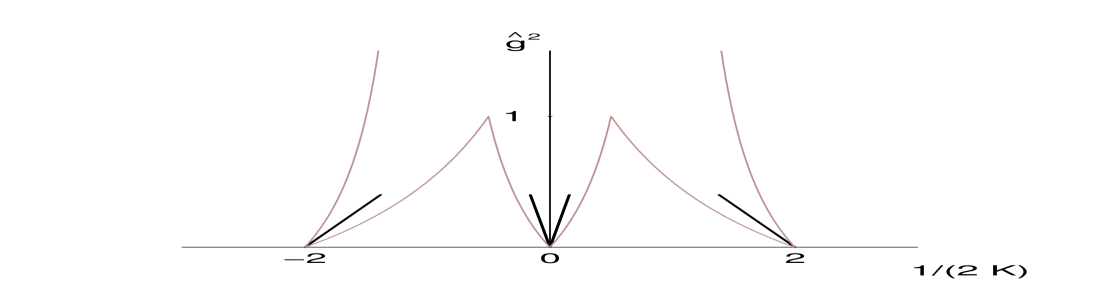
Figure 1: The phase diagram for the Gross-Neveu model in the weakly coupled region $g_{\phi}=g_{\pi}=g$ (to ${\cal{O}}({g}^{2})$) (dark lines) and a schematic representation of the expected Aoki phase diagram (light curves).

The actual phase diagram for weakly coupling is pictured in Fig. 1 for $g_{\phi}=g_{\pi}=g$ (dark lines). The lighter curves are a schematic representation of the expected full phase diagram. One sees the degeneracy of the central free fermion critical point is lifted and two critical lines emerge in the presence of weak bosonic coupling. These are the lines corresponding to the central cusp in Aoki’s phase diagram. From (5.15), the central cusp can only be made vanish at this order, in the unphysical situation of imaginary couplings. The Aoki phase does not yet emerge to ${\cal{O}}({{g}}^{2})$ from the left- and rightmost free critical points.

In the free case, the zeroes and hence the critical points are invariant under momentum inversion $p_{\mu}\rightarrow-p_{\mu}$, corresponding to a rotation in space-time. While this degeneracy is lifted at finite size in the interacting case, it is recovered in the limit of infinite volume. In that limit, the free zeroes and critical points are also invariant under the parity transformation $p_{1}\leftrightarrow p_{2}$. This is no longer the case in the presence of interactions. Indeed, the inner pair of critical lines are interchanged under parity. The overall phase structure, however, remains the same.

The situation is similar to the two dimensional Potts model. There, the partition function is invariant under a duality transformation which exchanges the high and low temperature phases. The critical point is that which is invariant under that transformation. Here, the zeroes, and hence the partition function, are invariant under parity. The phase structure is also unchanged by parity. However, parity even and parity odd regions of the phase diagram are interchanged.

6 Conclusions

A new type of weak coupling expansion appropriate for Wilson fermionic lattice field theories has been developed. This expansion is multiplicative, but recovers the standard additive expansion. Its multiplicative form allows the Lee-Yang zeroes of the weakly coupled theory to be extracted in a natural way. These zeroes, are protocritical points, which, if they impact on to the real hopping parameter axis, precipitate a phase transition there.

The expansion is applied to the single flavour lattice Gross-Neveu model to track the movement of zeroes and thereby the critical points in the presence of bosonic field variables. This model shares features with QCD, one of which is expected to be the existence of an Aoki phase.

Using the new weak coupling expansion, a phase diagram is obtained in the weakly coupled region which is consistent with that of Aoki. The widths of the Aoki cusps are analytically determined to second order in the couplings. The central cusp cannot be tuned away for real physical couplings. The lateral cusps do not yet emerge at this order. This is the answer to the question posed by Creutz in [16] for the single flavour Gross-Neveu model.

Finally, while the full phase structure is unaltered by a parity transformation, such an operation has the effect of exchanging the critical lines forming the inner Aoki cusp.

References

• [1] S. Hands, A. KociΔ‡ and J.B. Kogut, Ann. Phys. 224 (1993) 29; S. Hands, S. Kim and J.B. Kogut Nucl. Phys. B 442 (1995) 364.
• [2] N. Kawamoto, Nucl. Phys. B 190 (1981) 617.
• [3] S. Aoki, Phys. Rev. D, 30 (1984) 2653; Nucl. Phys. B 314 (1989) 79.
• [4] S. Aoki, Phys. Rev. D 33 (1986) 2399; ibid. 34 (1986) 3170; Phys. Rev. Lett. 57 (1986) 3136.
• [5] T. Eguchi and R. Nakayama, Phys. Lett. B 126 (1983) 89.
• [6] S. Aoki and A. Gocksch, Phys. Lett. B 231 (1989) 449; ibid. 243 (1990) 409; Phys. Rev D 45 (1992) 3845.
• [7] S. Aoki, S. Boettcher and A. Gocksch, Phys. Lett. B 331 (1994) 157.
• [8] K.M. Bitar and P.M. Vranas, Nucl. Phys. B (Proc.Suppl.) 42 (1995) 746.
• [9] S. Aoki, T. Kaneda and A. Ukawa, Phys. Rev. D 56 (1997) 1808; S. Aoki, Nucl. Phys. B (Proc. Suppl.) 60A (1998) 206.
• [10] K.M. Bitar, Nucl. Phys. B (Proc. Suppl.) 63 (1998) 829.
• [11] S. Aoki, Prog. Theor. Phys. Suppl. 122 (1996) 179.
• [12] S. Sharpe and R.L. Singleton Jr., Phys. Rev. D 58 (1998) 074501; Nucl. Phys. B (Proc.Suppl.) 73 (1999) 234.
• [13] R. Kenna, C. Pinto and J.C. Sexton, Nucl. Phys. B (Proc. Suppl.) 83 (2000) 667; e-Print Archive: hep-lat/0101005 (to be published in Phys. Lett. B).
• [14] K.M. Bitar and P.M. Vranas, Phys. Lett. B 327 (1994) 101; Nucl. Phys. B (Proc.Suppl.) 34 (1994) 661.
• [15] K.M. Bitar, Phys. Rev. D 56 (1997) 2736; K.M. Bitar, U.M. Heller and R. Narayanan, Phys. Lett B 418 (1998) 167; R.G. Edwards, U.M. Heller, R. Narayanan and R.L. Singleton Jr., Nucl. Phys. B 518 (1998) 319.
• [16] M. Creutz, e-Print Archive: hep-lat/9608024 (Talk given at Brookhaven Theory Workshop on Relativistic Heavy Ions, Upton, NY, 8-19 Jul 1996); e-Print Archive: hep-lat/0007032.
• [17] D.J. Gross and A. Neveu, Phys. Rev. D 10 (1974) 3235.
• [18] Y. Nambu and G. Jona-Lasinio, Phys. Rev. 122 (1961) 345.
• [19] S. Aoki and K. Higashijima, Prog. Theor. Phys. 76 (1986) 521.
• [20] T. Izubuchi, J. Noaki and A. Ukawa, Phys. Rev. D 58 (1998) 114507; Nucl. Phys. B (Proc. Suppl.) 73 (1999) 483.
• [21] N.D. Mermin and H. Wagner, Phys. Rev. Lett. 22 (1966) 1133.
• [22] R. Kenna and A.C. Irving Phys. Lett. B 351 (1995) 273; Nucl. Phys. B 485 (1997) 583; A.C. Irving and R. Kenna Phys. Rev. B 53 (1996) 11568.
• [23] T.D. Lee and C.N. Yang, Phys. Rev. 87 (1952) 404; ibid. 410.
• [24] M.E. Fisher, Suppl. Prog. Theor. Phys. 69 (1980) 14.