Non-perturbative Renormalisation of Domain Wall Fermions: Quark Bilinears

Abstract

We find the renormalisation coefficients of the quark field and the flavour non-singlet fermion bilinear operators for the domain wall fermion action, in the regularisation independent (RI) renormalisation scheme. Our results are from a quenched simulation, on a $16^{3}\times 32$ lattice, with $\beta=6.0$ and an extent in the fifth dimension of $16$. We also discuss the expected effects of the residual chiral symmetry breaking inherent in a domain wall fermion simulation with a finite fifth dimension, and study the evidence for both explicit and spontaneous chiral symmetry breaking effects in our numerical results. We find that the relations between different renormalisation factors predicted by chiral symmetry are, to a good approximation, satisfied by our results and that systematic effects due to the (low energy) spontaneous chiral symmetry breaking and zero-modes can be controlled. Our results are compared against the perturbative predictions for both their absolute value and renormalisation scale dependence.

I Introduction

Renormalisation of lattice operators is an essential ingredient needed to deduce physical results from numerical simulations. In contrast with the determination of hadronic masses, physical matrix elements can be determined only if the normalisation of the appropriate lattice operators can be related to that of the corresponding continuum operators, conventionally specified perturbatively at short distances. In principle, lattice perturbation theory may be used to establish this connection. However, lattice perturbation theory converges slowly and the expansion parameter, the square of the lattice coupling evaluated at the lattice scale, $g(a)^{2}$, decreases only as an inverse power of $\ln(a)$. This makes systematic improvement of perturbative results essentially impossible. This convergence may be improved when, following ideas from continuum perturbation theory [1], a renormalised or ”boosted” [2] coupling rather than the bare coupling is used as an expansion parameter. Even so, considerable arbitrariness remains, and in general it is extremely difficult to go beyond one loop order in such calculations. To overcome these difficulties, Martinelli ${\it et.al.}$ [3] have proposed a promising non-perturbative renormalisation procedure. This method has been previously used to determine renormalisation coefficients for various operators using the Wilson [4, 5, 6, 7] and staggered actions [8]. The purpose of this work is to study the application of this technique to the renormalisation of the quark field and flavour non-singlet fermion bilinear operators for the domain wall fermion action.

Domain wall fermions [9, 10, 11] provide an action, that at the expense of introducing a fifth dimension, has a low energy theory with excellent chiral properties while at the same time preserving exact flavour symmetry. These good chiral properties lead to a suppression of the possible dimension five terms in the long-distance effective Lagrangian implying that domain wall fermions define a lattice version of QCD which is off-shell improved to ${\cal O}(a^{2})$. As we will see, these domain wall off-shell Greens functions show remarkably reduced lattice artifacts. A study of operator renormalisation coefficients for this action is useful, both because these numbers are needed for use in practical calculations of physical quantities [12] and because it provides an excellent test of the chiral properties of the domain wall fermion action in practical simulations. In fact, we find that domain wall fermions perform quite well for non-perturbative renormalisation with negligible contributions from explicit chiral symmetry breaking. This finding is in good agreement with recent work on the chiral limit of quenched QCD with domain wall fermions [12, 13].

Careful operator normalisation is especially important for the domain wall fermion method. As is reviewed in Section III A, the interpolating field conventionally used to create and destroy the physical modes is exactly localised in the fifth-dimension on the right and left walls. Since the actual physical modes extend somewhat into the fifth dimension, the overlap between the interpolating field and the physical modes will be smaller than one. This implies a wave function renormalisation factor $(Z_{q})$ which differs from one even in the case of free fields. For the eigenvectors corresponding to the smallest 19 Dirac eigenvalues examined in the quenched, $\beta=6.0$ calculation of Ref. [12], this overlap typically varies between 75 and 85%. Fortunately, the non-perturbative methods employed here [3] precisely include these effects.

We begin in Section II with a brief summary of the main issues involved in applying the non-perturbative renormalisation method. In Section III, we give the domain wall fermion action and discuss the Ward-Takahashi identities it obeys. Section IV builds on this base to constrain the ways in which explicit chiral symmetry breaking terms may enter low energy matrix elements calculated using domain wall fermions. In Section V we give the details of our lattice simulations. Section VI describes the renormalisation of the quark propagator, and in Section VII we introduce the quark bilinears and compute their renormalisation on the lattice in the regularisation independent scheme. After removing expected non-perturbative pole terms, we look for effects of explicit chiral symmetry breaking and find that they are negligible. In Section VIII, we avail ourselves of the axial Ward-Takahashi identity again to compute the quark wave function renormalisation from the conserved vector and partially conserved axial-vector currents. In Section IX we calculate the renormalisation of the non-conserved, local axial current from a ratio of its hadronic matrix element to the hadronic matrix element of the partially conserved axial current and find good agreement with the results of Section VII. In Section X we convert the renormalisation coefficients to renormalisation group invariant quantities by dividing out the renormalisation group running. In Section XI we discuss the calculation of the quark wavefunction renormalisation from the propagator.

After comparing our non-perturbative results with recent perturbative calculations in Section XII, we end with our conclusions. The details of the exact conventions and equations used for the perturbative running and matching are relegated to appendices.

II Non-Perturbative Renormalisation

In the following the method of non-perturbative renormalisation introduced in Ref. [3] will be studied. This method uses a renormalisation scheme that is defined by a set of conditions that mandate the renormalised values of the operators of interest between external quark states, in a fixed gauge, at large virtualities. As such these conditions may be expressed in any regularisation scheme (and so this scheme is known as the regularisation independent (RI) scheme). In particular this allows the renormalisation factors to be defined in the lattice regularisation, opening the way for renormalisation factors to be directly calculated in numerical lattice simulations.

While calculating renormalisation factors from lattice simulations neatly avoids the need to perform analytic calculations using lattice perturbation theory, which are both challenging and poorly behaved, doing so introduces several issues that must be considered:

• Calculating the matrix elements of the operators of interest between external quark states requires a fixed gauge to be used. This allows for the appearance of Gribov copies, possibly obscuring the required comparison with continuum perturbation theory where only the trivial copy appears. Earlier studies[14] of the size of Gribov noise in the calculation of a gauge invariant normalisation factor as a ratio of two gauge-variant amplitudes suggest this may not be an important difficulty for the parameters used here. However, in future work, this difficulty can be avoided by taking two steps: i) Impose the regularisation invariant normalisation condition in a sufficiently small physical volume that non-perturbative effects are suppressed. ii) Begin the Landau gauge fixing procedure from a configuration that is in a completely-fixed axial gauge. Taking these two precautions will insure that any effects of Gribov copies will be similar to other non-perturbative effects and will vanish as the comparison with perturbation theory is done at weaker and weaker coupling.

• Numerical simulations are performed with a finite lattice spacing. This provides a natural condition,

  $$|p|\ll\frac{1}{a}\,,$$ (1)

  over the momenta range for which a direct extraction of continuum quantities is possible.

• As the renormalisation factors are determined in a non-perturbative calculation the contributions of propagating mesons, and in particular pseudo-Goldstone bosons, must be identified and removed. These effects may be reduced by working at high momenta, with a natural condition for the absence of significant deviations being

  $$\Lambda_{QCD}\ll|p|\,.$$ (2)

Taking the last two points together suggests that this technique relies on the existence of a “window” of momenta,

$$\Lambda_{QCD}\ll|p|\ll\frac{1}{a}\,,$$ (3)

for which the predictions of continuum perturbation theory should correctly describe the form of the lattice data. In practical simulations however, it has been found that the effects of deviations due the violations of both these inequalities must be taken into account [4, 15, 7].

Fortunately, near either edge of this window, the form of deviations from perturbative behaviour may be predicted. In the case of momenta too low, the initial corrections may be described by an expansion in terms of momentum-suppressed condensate terms by use of the operator product expansion (OPE). In turn, the first corrections to continuum-like behaviour may be taken into account in terms of an expansion in the lattice spacing, $a$.

Another trivial consequence of the restricted range of momenta available in current lattice simulations is the need for many phenomenological calculations to be composed of continuum perturbation theory calculations at high scales, that are then run down to scales accessible on the lattice and combined with the lattice result. As the majority of the existing calculations for the continuum perturbative results use renormalisation schemes that may only be defined when using dimensional regularisation (such as the $\overline{MS}$ scheme), perturbative matching calculations between these schemes and the ones that may be defined in the lattice regularisation need to be performed.

III Domain Wall Fermions

In this section the domain wall fermion formulation, as used in our simulations, will be reviewed.

A Action

The domain wall fermion (DWF) method is a promising new approach to lattice QCD introduced in Ref. [10], which, at the expense of introducing an extra, discrete, non-gauge dimension, provides drastically improved chiral properties at finite lattice spacing while preserving exact symmetry under vectorial flavour rotations. This is achieved by using an action in the fifth dimension that is asymmetric between the left-handed and right-handed components of the fermion field. Denoting the fifth co-ordinate as $s$, with

$$s\in 0,\cdots,L_{s}-1\,,$$ (4)

the massless action may be written as

$$S_{{\rm fermion}}(m_{f}=0) = -\sum_{x,s}\overline{\Psi}_{x,s}\left\{-\gamma_{\mu}\frac{1}{2}\left(\nabla^{+}_{\mu}+\nabla^{-}_{\mu}\right)\right.$$ (6)

$$\left.+\left[\frac{1}{2}\nabla^{-}_{\mu}\nabla^{+}_{\mu}+M_{5}\right]+P_{L}\partial^{+}_{5}-P_{R}\partial^{-}_{5}\right\}\Psi_{x,s}\,,$$

with

$$Z=\int[dU][d\overline{\Psi}d\Psi]\exp\left(-S_{{\rm gauge}}-S_{{\rm fermion}}\right)\,.$$ (7)

In Eqs. 6 and 7 $\Psi_{x,s}$ is the fermionic field, $U_{\mu}(x)$ is the gauge field and

$$S_{{\rm gauge}}=\beta\sum_{P}\left(1-\frac{1}{3}\mathrm{Re\,Tr}\left[U_{P}\right]\right)\,,$$ (8)

with $\beta=6/g_{0}^{2}$ and $g_{0}$ is the bare lattice coupling. The projectors for the left and right-handed spinors are defined as,

$$P_{L} = \frac{1}{2}\left(1-\gamma^{5}\right)$$ (9)

$$P_{R} = \frac{1}{2}\left(1+\gamma^{5}\right)\,.$$ (10)

The notation $\nabla^{\pm}_{\mu}$ has been used to denote the discrete forward/backward covariant derivatives:

$$\nabla^{+}_{\mu}\psi_{x} = \left[U_{\mu}(x)\psi_{x+\mu}-\psi_{x}\right]$$ (11)

$$\nabla^{-}_{\mu}\psi_{x} = \left[\psi_{x}-U^{\dagger}_{\mu}(x-\mu)\psi_{x-\mu}\right]\,,$$ (12)

and $\partial^{\pm}_{\mu}$ represents the corresponding derivative with no gauge term. For the case of the derivative in the fifth dimension, $\partial^{\pm}_{5}$, the domain wall is implemented by giving the derivative hard boundaries. For example a one-dimensional $\partial_{5}^{+}$ acting on a space with four points may be written in matrix form as

$$\partial_{5}^{+}\left(\begin{array}[]{c}\Psi_{x,0}\\ \Psi_{x,1}\\ \Psi_{x,2}\\ \Psi_{x,3}\\ \end{array}\right)=\left(\begin{array}[]{cccc}-1&1&0&0\\ 0&-1&1&0\\ 0&0&-1&1\\ 0&0&0&-1\\ \end{array}\right)\left(\begin{array}[]{c}\Psi_{x,0}\\ \Psi_{x,1}\\ \Psi_{x,2}\\ \Psi_{x,3}\\ \end{array}\right)\,.$$ (13)

It should be noted that the action in Eq. 6 is actually the hermitian conjugate of the action proposed in Ref. [10]. This change was made for practical reasons related to compatibility with the existing Wilson operator implementation for the QCDSP machine.

In the free theory, for $0<M_{5}<2$, the effect of this is to produce a spectrum with one light fermionic mode, with exact chiral symmetry in the $L_{s}\rightarrow\infty$ limit, and $16L_{s}-1$ heavy modes. The wavefunction of this light mode has its right-handed component concentrated on the wall at $s=L_{s}-1$ and its left-handed component on the wall at $s=0$. This light fermion mode may be studied by introducing an interpolating operator of the form [16]

$$q_{x} = P_{L}\Psi_{x,0}+P_{R}\Psi_{x,L_{s}-1}$$ (14)

$$\overline{q}_{x} = \overline{\Psi}_{x,0}P_{R}+\overline{\Psi}_{x,L_{s}-1}P_{L}\,.$$ (15)

The above considerations also naturally lead to the introduction of an explicit mass term to the action of the form

$$S_{{\rm fermion}}(m_{f})=S_{{\rm fermion}}(m_{f}=0)+\sum_{x}\,m_{f}\,\overline{q}q\,,$$ (16)

where $m_{f}$ is the bare quark mass. In the free case, this leads to a spectrum with one light fermion of mass

$$M_{5}\left(2-M_{5}\right)\left(m_{f}+\left(1-M_{5}\right)^{L_{s}}\right)\,.$$ (17)

Note that in the $L_{s}\rightarrow\infty$ limit this is proportional to $m_{f}$, while for finite $L_{s}$ there remains a residual mass, $m_{{\rm res}}$, that acts as an additive renormalisation to $m_{f}$.

However, the properties of domain wall fermions in the presence of gauge fields is a much more difficult question. In particular while the form of the mass of the light mode is expected to be proportional to $m_{f}+m_{\mathrm{res}}$, the dependence of $m_{\mathrm{res}}$ on $L_{s}$ must be determined. Perturbative calculations [17, 18, 19, 20, 21] have shown that the existence of the light mode is stable to small perturbations and that this mode has all chiral symmetry breaking proportional to $m_{f}$ as $L_{s}\rightarrow\infty$. These studies also highlight several issues that must be considered when undertaking numerical simulations:

1. The dependence of $m_{{\rm res}}$ on $L_{s}$ may no longer be of the simple exponential form shown in Eq. 17.

2. $M_{5}$ undergoes a strong additive renormalisation. This is understandable, as the five dimensional problem has no approximate chiral symmetry to protect it.

Indeed, extensive numerical studies in the quenched approximation [12, 13] have shown that the $L_{s}$ dependence of $m_{\mathrm{res}}$ does not fit a single exponential in the range $L_{s}=12\rightarrow 48$ for lattices with the same lattice spacing ($a=0.520{\rm GeV}^{-1}$) as the results in this paper. For $L_{s}=16$, the value used in this work, $m_{\mathrm{res}}$ was found to be $\sim 4{\rm MeV}$ in the $\overline{MS}$ scheme at $2\mathrm{GeV}$ [12]. The strong additive renormalisation of $M_{5}$ requires that an input value be chosen numerically so that a single light mode forms and that its decay in $L_{s}$ is as rapid as possible. It has been found that for even coarser lattices than used here such a choice can be made [22, 12].

B Lattice Ward-Takahashi Identities

For the purpose of analysing the consequences of the symmetries of the action, it is convenient to introduce an extended mass term, $M$, with flavour structure such that the mass term reads

$$\overline{q}_{L}M^{\dagger}q_{R}+\overline{q}_{R}Mq_{L}\,,$$ (18)

and so the mass term is invariant under a transformation of the quark fields and the mass matrix $M$ of the form

$$q_{L} \rightarrow U_{L}q_{L}$$ (19)

$$q_{R} \rightarrow U_{R}q_{R}$$ (20)

$$M \rightarrow U_{R}\,M\,U_{L}^{\dagger}.$$ (21)

Following Ref. [16], on a finite lattice, an exact vector Ward-Takahashi identity may be derived by considering transformations of the 5-dimensional fermion field, $\Psi$, such that

$$\delta_{V}\Psi_{x,s} = i\epsilon_{x}^{a}T^{a}\Psi_{x,s}$$ (22)

$$\delta_{V}\overline{\Psi}_{x,s} = -i\epsilon_{x}^{a}\overline{\Psi}_{x,s}T^{a}\,,$$ (23)

where $\left\{T^{a}\right\}$ is the set of hermitian traceless matrices acting on $SU(N_{f})$ flavour-space. This leads to an exact Ward-Takahashi identity that reads:

$$-\partial_{\mu}^{-}\langle{\cal V}_{\mu}^{a}(z)O(x_{1},\cdots,x_{n})\rangle$$ (24)

$$+\langle\overline{q}\left[M,T^{a}\right]q(z)\,O(x_{1},\cdots,x_{n})\rangle = -i\langle\delta^{a}O(x_{1},\cdots,x_{n})\rangle\,,$$ (25)

where

$${\cal V}_{\mu}^{a}(x) = \frac{1}{2}\sum_{s}\left(\overline{\Psi}_{x+\mu,s}\left(1+\gamma_{\mu}\right)U^{\dagger}_{x,\mu}T^{a}\Psi_{x,s}\right.$$ (27)

$$\left.-\overline{\Psi}_{x,s}\left(1-\gamma_{\mu}\right)U_{x,\mu}T^{a}\Psi_{x+\mu,s}\right)\,.$$

For the case of axial transformations the analogous choice is a transformation of the form:

$$\delta_{A}\Psi_{x,s} = i\epsilon_{x,s}^{a}T^{a}\Psi_{x,s}$$ (28)

$$\delta_{A}\overline{\Psi}_{x,s} = -i\epsilon_{x,s}^{a}\overline{\Psi}_{x,s}T^{a}\,,$$ (29)

with

$$\epsilon_{x,s}^{a}=\left\{\begin{array}[]{rc}\epsilon_{x}^{a}&0\leq s<L_{s}/2\\ -\epsilon_{x}^{a}&L_{s}/2\leq s<L_{s}\,.\end{array}\right.$$ (30)

This leads to a Ward-Takahashi identity of the form

$$-\partial_{\mu}^{-}\langle{\cal A}_{\mu}^{a}(z)O(x_{1},\cdots,x_{n})\rangle$$ (31)

$$+\langle\overline{q}\left\{M,T^{a}\right\}\gamma_{5}q(z)\,O(x_{1},\cdots,x_{n})\rangle$$ (32)

$$+2\langle J_{5q}^{a}\,O(x_{1},\cdots,x_{n})\rangle = -i\langle\delta^{a}_{A}O(x_{1},\cdots,x_{n})\rangle\,,$$ (33)

where

$${\cal A}^{a}_{\mu} = \frac{1}{2}\sum_{s}\mathrm{sign}\left(s-\frac{L_{s}-1}{2}\right)\left(\overline{\Psi}_{x+\mu,s}\left(1+\gamma_{\mu}\right)U^{\dagger}_{x,\mu}T^{a}\Psi_{x,s}\right.$$ (35)

$$\left.-\overline{\Psi}_{x,s}\left(1-\gamma_{\mu}\right)U_{x,\mu}T^{a}\Psi_{x+\mu,s}\right)$$

$$J_{5q}^{a} = -\overline{\Psi}_{x,L_{s}/2-1}P_{L}T^{a}\Psi_{x,L_{s}/2}+\overline{\Psi}_{x,L_{s}/2}P_{R}T^{a}\Psi_{x,L_{s}/2-1}\,.$$ (36)

Therefore, in contrast to the previous case, the axial current is not exactly conserved. This is necessary both to provide a mechanism for physical terms due to the $U(1)_{A}$ axial anomaly to enter the calculated amplitudes and also to allow for explicit chiral symmetry breaking contributions at finite $L_{s}$. The situation is analogous to that for Wilson fermions [23], where the role of $J_{5q}^{a}$ is played by the chiral variation of the Wilson term, except that the contributions from $J_{5q}^{a}$ are expected to tend to zero as $L_{s}\rightarrow\infty$ in the present case [16]. The form of the contributions from $J_{5q}^{a}$ will be further discussed in the next section.

IV Operator Mixing and Chiral Symmetry

The major attraction of the domain wall fermion formalism is its ability to decrease the size of chiral symmetry breaking by increasing the parameter $L_{s}$, the distance between the two four-dimensional lattice boundaries to which the left and right chiral modes are bound. However, it is often impractical or inefficient to choose such a large value of $L_{s}$ that all chiral symmetry breaking effects from mixing between these walls can be neglected. Thus, it is important to characterise the effects of this chiral symmetry breaking and in this section we will determine how it can effect the low energy physics of lattice QCD. As we will see, this can be done as either an expansion in the size of the wall-mixing effects, which for simplicity we will denote by ${\cal O}(e^{-\alpha L_{s}})$ although the exact $L_{s}$ dependence may be different, and/or as an expansion in the lattice spacing $a$.

This analysis is easily made by starting with the interpretation of chiral symmetry proposed by Furman and Shamir [16]. Here one identifies the full $SU(N_{f})_{L}\otimes SU(N_{f})_{R}$ chiral symmetry of the continuum theory as the independent $SU(N_{f})$ rotation of the fermion fields defined on the left- and right-hand halves of the five-dimensional lattice:

$$\begin{array}[]{rcll}\Psi(x,s)&\rightarrow&U_{L}\Psi(x,s)&\;\;0\leq s\leq L_{s}/2-1\\ \Psi(x,s)&\rightarrow&U_{R}\Psi(x,s)&\;\;L_{s}/2\leq s\leq L_{s}-1\,,\\ \end{array}$$ (37)

where $U_{L}$ and $U_{R}$ are $N_{f}\times N_{f}$ special unitary matrices belonging to the left and right factors of $SU(N_{f})_{L}\otimes SU(N_{f})_{R}$. From Eq. 14 it is clear that this transformation will act on the four-dimensional quark fields as a standard element of the full chiral symmetry.

Of course, the transformation in Eq. 37, whose generators are given in Eq. 29 and Eq. 23, cannot be an exact symmetry of the five-dimensional theory as the derivative terms in the fifth dimension, taken collectively, couple the left and right hand walls and prevent such independent rotations of this single, five-dimensional field. However, in the low energy sector of the theory this symmetry can be quite good. The physical, chiral modes which survive at low energy are expected to be exponentially bound to the walls with an overlap that is suppressed as $L_{s}$ increases. The higher energy modes which can propagate freely between the walls are all far off-shell with propagators which are necessarily also exponentially suppressed at long distances, especially for the large distance $L_{s}$.

In order to characterise the effects of this controlled symmetry breaking that comes from communication between the walls, we will generalise somewhat the Dirac domain wall fermion operator of Shamir given in Eq. 16. We will introduce a special-unitary, flavour matrix $\Omega$ in the derivative term joining the four-dimensional planes $s=L_{s}/2-1$ and $s=L_{s}/2$. Thus, we will modify Eq. 6 by adding the term:

$$S_{\Omega}=-\sum_{x}\left\{\overline{\Psi}_{x,L_{s}/2-1}P_{L}\left(\Omega^{\dagger}-1\right)\Psi_{x,L_{s}/2}+\overline{\Psi}_{x,L_{s}/2}P_{R}\left(\Omega-1\right)\Psi_{x,L_{s}/2-1}\right\}\,.$$ (38)

If we include the transformation of the matrix $\Omega$,

$$\Omega\rightarrow U_{R}\,\Omega\,U_{L}^{\dagger}\,,$$ (39)

this generalised domain wall Dirac operator will now possess exact chiral symmetry. Note, a comparison with Eq. 21 shows that $\Omega$ transforms “like a mass term”.

Thus, if we examine this generalised theory that includes the chiral matrix $\Omega$, all amplitudes will become functions of $\Omega$ but will exactly obey the chiral symmetry described by Eq. 37 and Eq. 39. Therefore, we need only understand how the matrix $\Omega$ will enter the low energy Green’s functions of interest to determine in a precise way the transformation properties of the chiral symmetry breaking induced by mixing between the walls.

To zeroth order in $e^{-\alpha L_{s}}$, the fermion degrees of freedom will remain bound to the walls and propagation from one wall to the other can be neglected. In such circumstances, the matrix $\Omega$ which is introduced at a point mid-way between the walls cannot enter, the amplitude will be independent of $\Omega$ and hence naively invariant under the full $SU(N_{f})_{L}\otimes SU(N_{f})_{R}$ chiral symmetry. To the next order, $\propto e^{-\alpha L_{s}}$, we expect phenomena which involve a single propagation between $s=0$ and $s=L_{s}-1$. Thus, the matrix $\Omega$ should enter linearly in such amplitudes.

An important application of this analysis is to constrain the form of the effective continuum action which gives amplitudes that agree with those of the domain wall theory through a given order in the lattice spacing. To leading order in the lattice spacing, this effective Lagrangian has the standard continuum form. The above analysis requires that the mass term in this leading order effective Lagrangian must have the form:

$$Z_{m}m_{f}\overline{\psi}\psi+c\left\{\overline{\psi}\Omega^{\dagger}P_{R}\psi+\overline{\psi}\Omega P_{L}\psi\right\}\,,$$ (40)

where $c$ is a constant with the dimensions of mass. Here the field $\psi$ represents a conventional continuum multiplet of quark fields and all quantities carry their physical dimensions. The first piece is the normal chiral symmetry breaking introduced by the input mass $m_{f}$. The second comes from mixing between the walls and is required by the extended symmetry of Eq. 37 and Eq. 39 to be linear in $\Omega$. Thus, this induced mass term can occur to first order in the mixing between the walls, permitting $c\propto e^{-\alpha L_{s}}/a$. With the conventional choice of Shamir, $\Omega_{a,b}=\delta_{a,b}$, the second term in Eq. 40 reduces to our usual residual mass term with $am_{\rm res}\approx 10^{-3}$ [12].

In a similar fashion the ${\cal O}(a)$ effective Lagrangian will contain a clover term induced by mixing between the walls, again to first order in $e^{-\alpha L_{S}}$, since it also has the permitted $SU(N_{f})_{L}\otimes SU(N_{f})_{R}$ chiral structure:

$$ac_{1}\,\left\{\overline{\psi}\sigma_{\mu\nu}F_{\mu\nu}\Omega^{\dagger}P_{R}\psi+\overline{\psi}\sigma_{\mu\nu}F_{\mu\nu}\Omega P_{L}\psi\right\}.$$ (41)

where $c_{1}\propto e^{-\alpha L_{s}}$ is $\cal{O}$($am_{\mathrm{res}}$). Thus, such a term is suppressed both by the lattice spacing and by the smallness of $m_{\mathrm{res}}$.

If we extend these considerations to ${\cal O}(a^{2})$ terms in the effective Lagrangian, we can conclude that a four-fermi operator of the form

$${c_{2}a^{2}}(\overline{\psi}\psi)(\overline{\psi}\psi)\,,$$ (42)

where $c_{2}$ is a constant, cannot occur to order $e^{-\alpha L_{s}}$. Since this operator will become a chiral singlet only when contracted with two powers of the matrix $\Omega$ or one power of $\Omega$ and one powers of the mass matrix $M$ of Eq. 18, the coefficient of such an operator must contain a double suppression $c_{2}\propto e^{-2\alpha L_{s}}$ or a further factor of $m_{f}$.

V Simulation Details

In the following discussions much use will be made of the momentum space quark propagator in Landau gauge. The first step in calculating this quantity is to fix the gauge. We implement Landau gauge fixing by iteratively sweeping over all lattice sites, maximising the functional

$$\sum_{x,\mu}\left[{\rm Tr}\left(U_{\mu}(x)+U_{\mu}^{\dagger}(x)\right)\right]\,.$$ (43)

At each lattice site we determine a gauge transformation matrix, $g(x)$, which increases the value of Eq. 43. The maximum is achieved when

$$\sum_{x}{\rm Tr}\left[B(x)B^{\dagger}(x)\right]$$ (44)

is zero, where

$$B(x)=A(x)-A^{\dagger}(x)-\frac{1}{3}{\rm Tr}(A-A^{\dagger})$$ (45)

$$A(x)=\sum_{\mu}\left[\tilde{U}_{\mu}^{\dagger}(x)+\tilde{U}_{\mu}(x-\mu)\right]$$ (46)

and

$$\tilde{U}_{\mu}(x)=g(x)U_{\mu}(x)g^{\dagger}(x+\mu)\,.$$ (47)

In practice we stop when the quantity in Eq. 44 is smaller than $10^{-8}$.

On this gauge-fixed configuration the quark propagator, $S\left(x,0\right)$, from one source, denoted as $0$, to all possible sinks is then calculated. A discrete Fourier transform is then performed over the sink positions giving,

$$S\left(p,0\right)=\sum_{x}\exp\left(-ip^{{\rm latt}}\cdot x\right)S\left(x,0\right)\,,$$ (48)

with

$$p^{\mathrm{latt}}_{\mu}=\frac{2\pi}{L_{\mu}}n_{\mu}\,,$$ (49)

where $\mu$ is one of $x$,$y$,$z$ or $t$ and $n_{\mu}$ may in principle lie in the range $0\rightarrow L_{\mu}-1$. In practice, however, only a subset of this range is used.

Unless otherwise stated all the data that will be presented is from calculations on a $16^{3}\times 32\times 16$ lattice (where the last number refers to the extent of the lattice in the fifth dimension). The simulation was performed at $\beta=6.0$ with $2000$ heatbath sweeps between every configuration and with $2000$ thermalisation sweeps performed at the outset. In total $142$ configurations were generated. For this lattice size the momentum range was restricted to those momenta for which $n_{\mu}=0,1,2$ for $\mu=x,y,z$ and $n_{t}=0,1,2,3$. Quark propagators for $5$ bare masses, $m_{f}=0.01$, 0.02, 0.03, 0.04 and 0.05 were calculated all using $M_{5}=1.8$.

The results will often be quoted against the square of the absolute momentum, where this refers to the Euclidean inner product of the momentum defined in Eq. 49. To be more specific

$$\left(ap\right)^{2}=\sum_{\mu}p^{\mathrm{latt}}_{\mu}\,p^{\mathrm{latt}}_{\mu}\,,$$ (50)

where $p$ is dimensionful.

VI The Renormalised Propagator

Before we treat the more complicated situation of the fermion bilinears it is necessary to first consider the renormalisation of the quark propagator. Neglecting, for the moment, potential contributions from lattice artifacts the renormalised quark field may be defined as

$$q_{\mathrm{ren}}(x)=Z_{q}^{\frac{1}{2}}q_{0}(x)\,.$$ (51)

If we similarly introduce a renormalised mass, defined by

$$m_{\mathrm{ren}}=Z_{m}m_{0}\,,$$ (52)

where $m_{0}$ represents a generic multiplicatively renormalised bare mass, then the renormalised propagator may be written

$$S_{\mathrm{ren}}\left(p,m_{\mathrm{ren}}\right)=Z_{q}S_{0}\left(p,m_{0}\right)|_{m_{0}=m_{\mathrm{ren}}/Z_{m}}\,.$$ (53)

Both $Z_{q}$ and $Z_{m}$ are fixed in the RI scheme by requiring that the renormalised propagator obey the Euclidean space relations

$$\lim_{m_{\mathrm{ren}}\rightarrow 0}-\frac{i}{12}\mathrm{Tr}\left(\frac{\partial S^{-1}_{\mathrm{ren}}}{\partial\mathchoice{\ooalign{$\hfil\displaystyle\mkern 1.0mu/\hfil$\crcr$\displaystyle p$}}{\ooalign{$\hfil\textstyle\mkern 1.0mu/\hfil$\crcr$\textstyle p$}}{\ooalign{$\hfil\scriptstyle\mkern 1.0mu/\hfil$\crcr$\scriptstyle p$}}{\ooalign{$\hfil\scriptscriptstyle\mkern 1.0mu/\hfil$\crcr$\scriptscriptstyle p$}}}(p)\right)_{p^{2}=\mu^{2}}=1$$ (54)

$$\lim_{m_{\mathrm{ren}}\rightarrow 0}\frac{1}{12\,m_{\mathrm{ren}}}\mathrm{Tr}\left(S^{-1}_{\mathrm{ren}}(p)\right)_{p^{2}=\mu^{2}}=1\,.$$ (55)

While Eq. 54 and Eq. 55 seem to give a simple and appealing way to calculate $Z_{q}$ and $Z_{m}$ by directly applying them to the lattice propagators, the effect of both lattice artifacts and spontaneous chiral symmetry breaking must be considered.

Lattice actions with explicit chiral symmetry breaking require an additive renormalisation of the input mass, which may be taken into account for domain wall fermions by making the replacement

$$m_{0}\rightarrow m_{f}+m_{\mathrm{res}}\,,$$ (56)

in the equations above. However, the effects of lattice artifacts on the correct definition of the renormalised and improved quark field are more complicated. They have been studied in Ref. [24] for Wilson fermions, where it is noted that there are three terms that may mix with the definition at $\cal{O}$(a) in the lattice spacing, giving rise to an expression for the improved and renormalised quark field of

$$q_{\mathrm{ren}}=Z_{q}^{\frac{1}{2}}\left(1+b_{q}ma\right)\left\{1+a{c^{\prime}}_{q}\left(\mathchoice{\ooalign{$\hfil\displaystyle\mkern 1.0mu/\hfil$\crcr$\displaystyle D$}}{\ooalign{$\hfil\textstyle\mkern 1.0mu/\hfil$\crcr$\textstyle D$}}{\ooalign{$\hfil\scriptstyle\mkern 1.0mu/\hfil$\crcr$\scriptstyle D$}}{\ooalign{$\hfil\scriptscriptstyle\mkern 1.0mu/\hfil$\crcr$\scriptscriptstyle D$}}+m_{\mathrm{ren}}\right)+ac_{{\rm NGI}}\mathchoice{\ooalign{$\hfil\displaystyle\mkern 1.0mu/\hfil$\crcr$\displaystyle\partial$}}{\ooalign{$\hfil\textstyle\mkern 1.0mu/\hfil$\crcr$\textstyle\partial$}}{\ooalign{$\hfil\scriptstyle\mkern 1.0mu/\hfil$\crcr$\scriptstyle\partial$}}{\ooalign{$\hfil\scriptscriptstyle\mkern 1.0mu/\hfil$\crcr$\scriptscriptstyle\partial$}}\right\}q_{0}\,,$$ (57)

where $\hfil\textstyle\mkern 1.0mu/\hfil$ $\textstyle\partial$ may appear because the gauge is fixed. If such extra terms appear then conditions must be found that allow them to be subtracted from the bare quark field before Eq. 54 and Eq. 55 may be applied. In the context of simulations using $\cal{O}$(a) improved Wilson action at $\beta=6.0$ these terms have been found to give significant contributions to the form of the propagator [24]. In particular $c_{q}^{\prime}$ was found to be large. However, they all break chiral symmetry and so, following the arguments of Section IV, should be suppressed by a factor of $O(am_{{\rm res}})$ for simulations using domain wall fermions. As such, studying the form of the propagator provides an excellent test of the chiral properties of domain wall fermions.

The effects of spontaneous chiral symmetry breaking on the form of the propagator are well known [25, 26]. The most noticeable effect is that the trace of the inverse propagator picks up an extra contribution, which at lowest order in a power expansion in $1/p^{2}$ may be described as

$$\frac{1}{12}{\rm Tr}\left(S^{-1}_{\mathrm{ren}}(p)\right)=m_{\mathrm{ren}}+C_{1}\frac{\langle\overline{q}q\rangle}{p^{2}}+\cdots$$ (58)

where, at first order in perturbation theory, $C_{1}=4\pi\alpha_{s}/3$. Putting Eq. 58 and Eq. 57 together, the predicted form for the trace of the lattice quark propagator is

$$\frac{1}{12}\mathrm{Tr}\left(S_{latt}^{-1}(ap)\right) = \cdots+\frac{a^{3}\langle\overline{q}q\rangle}{(ap)^{2}}C_{1}Z_{q}$$ (61)

$$+\,Z_{m}Z_{q}\left\{am_{f}+am_{{\rm res}}\right\}$$

$$+\,2\left(c_{{\rm NGI}}Z_{q}-{c^{\prime}}_{q}\right)(ap)^{2}\,\,+\cdots\,,$$

where terms of $\cal{O}$($mc_{{\rm NGI}}$) have been neglected.

In Figure 1 we plot the left-hand side of Eq. 61 versus $(ap)^{2}$ for a variety of values for $m_{f}$. As can be seen, for domain wall fermions this quantity approaches a constant value for moderately large values of $(ap)^{2}$. Also, it is encouraging that while at low momenta the effects of spontaneous chiral symmetry are visible, there is no evidence to suggest appreciable effects from explicit chiral symmetry breaking. In particular, there is no evidence of a large additive mass renormalisation. This is visible in Figure 2, which shows the result of a linear extrapolation of the data to the point $m_{f}=0$. Figure 3 shows the slope of this extrapolation, which from Eq. 61 is $Z_{m}Z_{q}$ at large $(ap)^{2}$.

A Extracting $Z_{q}$ from the Propagator

The extraction of $Z_{q}$ from the propagator via Eq. 54 is numerically challenging due to the need for a discrete derivative to be calculated. A much simpler method [3], is to calculate

$${Z^{\prime}}_{q}=-i\frac{1}{12}\sum_{\mu}\frac{ap_{\mu}}{(ap)^{2}}\mathrm{Tr}\left(\gamma_{\mu}S^{-1}_{\mathrm{latt}}(ap)\right)\,.$$ (62)

This quantity may then be related to $Z_{q}$ by a perturbative matching calculation performed in the continuum [27].

On the other hand, the use of ${Z^{\prime}}_{q}$ to determine $Z_{q}$ introduces significant $O(a^{2})$ errors through the choice of how the discretised momenta are defined. If we were to replace in Eq. 62 the definition of the lattice momentum in Eq. 49 by, for example,

$$\bar{p}_{\mu}=\frac{1}{a}\sin p_{\mu}a\,,$$ (63)

then the resulting ${Z^{\prime}}_{q}$ would differ from that given in Eq. 62 by $O(a^{2})$ because the trace includes an explicit factor of $p_{\mu}\gamma_{\mu}$. One can estimate the size of this error by using various definitions for the lattice momentum in the analysis. As will be shown later in Sec. XI, this uncertainty is roughly 10–20%. In Sections VIII and IX we introduce two methods for computing $Z_{q}$ which avoid this uncertainty.

VII Flavour Non-Singlet Fermion Bilinears

A Introduction

In the following the renormalisation of the flavour non-singlet fermion bilinear operators will be considered. To simplify notation explicit quark flavours ($u$ and $d$) will be used in the following equations. The most general fermion bilinear may be written as $\overline{u}\Gamma_{i}d$ with

$$\Gamma_{i}\in\left\{1,\gamma_{\mu},\gamma_{5},\gamma_{\mu}\gamma_{5},\sigma_{\mu\nu}\right\}\,,$$ (64)

where $i$ represents whatever indices the gamma matrices have. The renormalised operator is defined as

$$\left[\overline{u}\Gamma d\right]_{{\rm ren}}=Z_{\Gamma}\left[\overline{u}\Gamma d\right]_{0}\,.$$ (65)

The factor $Z_{\Gamma}$ is fixed in the RI scheme by defining the unrenormalised, amputated vertex function

$$\Pi_{\Gamma,0}(p,q)=\frac{1}{V}\int d^{4}z\,d^{4}x_{1}\,d^{4}x_{2}\,e^{-ip.x_{1}+iq.x_{2}}\,\langle\,\left[\overline{u}\Gamma d\right]_{0}(z)\,u_{0}(x_{1})\,\overline{d_{0}}(x_{2})\,\rangle_{{\rm AMP}},$$ (66)

the corresponding renormalised, amputated vertex function

$$\Pi_{\Gamma,{\rm ren}}(p,q)={Z_{\Gamma}\over Z_{q}}\Pi_{\Gamma,0}(p,q)$$ (67)

and requiring that

$$\Lambda_{\Gamma_{i},\mathrm{ren}}(p,p)_{p^{2}=\mu^{2}}=\frac{1}{\mathrm{Tr}\left(\sum_{i}\Gamma_{i}\Gamma_{i}\right)}\mathrm{Tr}\left(\,\sum_{i}\Gamma_{i}\Pi_{\Gamma_{i},\mathrm{ren}}(p,p)\right)_{p^{2}=\mu^{2}}=1\,.$$ (68)

Note, the corresponding, unrenormalised vertex amplitude is defined by

$$\Lambda_{\Gamma,0}=\frac{1}{\mathrm{Tr}\left(\sum_{i}\Gamma_{i}\Gamma_{i}\right)}\mathrm{Tr}\left(\,\sum_{i}\Gamma_{i}\Pi_{\Gamma_{i},0}(p,p)\right)\,,$$ (69)

so that

$$\Lambda_{\Gamma_{i},\mathrm{ren}}(p,p)=\frac{Z_{\Gamma}}{Z_{q}}\Lambda_{\Gamma_{i},0}(p,p)\,.$$ (70)

While Eq. 70 completely defines a procedure for calculating a renormalisation factor for the bilinear operator of interest, practically we need to be able to use a renormalisation condition that allows us to match to perturbative calculations. In general the value of $\Lambda_{\Gamma_{i},0}(p,p)$ has contributions from intrinsically non-perturbative effects (such as those due to propagating pions) that perturbative calculations do not include. As we are interested in the value of the renormalisation factors in the perturbative regime we either apply the renormalisation condition at a high enough momenta such that the non-perturbative effects are suppressed, or remove such effects from the data and in the following that is what we will do. We will reserve the notation $Z_{i}$, $i\in\{q,S,P,T,A,V\}$ for the renormalisation factors in the perturbative regime.

B $Z_{A}$ and $Z_{V}$

A (partially) conserved current that is normalised in a fashion which is consistent with the usual Ward-Takahashi identities will undergo no renormalisation and the corresponding $Z_{\Gamma}$ will be unity. In particular, for domain wall fermions and the RI renormalisation scheme specified by Eqs. 54 and 68 and imposed at high-momentum, $\mu\gg\Lambda_{QCD}$, we expect

$$Z_{\cal A}=Z_{\cal V}=1.$$ (71)

However, on the lattice the (partially) conserved currents are not local and it is frequently more convenient to work with their local counterparts. Provided that these are related by a chiral transformation one still has

$$Z_{A}=Z_{V}\,.$$ (72)

This does not, however, mean that $\Lambda_{A}$ must equal $\Lambda_{V}$, and several mechanisms exist for splitting them away from each other at low energies.

Even if there are no significant effects from explicit chiral symmetry breaking, the effects of spontaneous chiral symmetry breaking must be taken into account. Consideration of the operator product expansion, to lowest order in powers of $1/p^{2}$, shows that $\Lambda_{A}$ and $\Lambda_{V}$ may get contributions from terms of the form

$$\frac{m_{\mathrm{ren}}^{2}}{p^{2}}$$ (73)

and

$$\frac{m_{\mathrm{ren}}\langle\overline{q}q\rangle}{p^{4}}\,.$$ (74)

Since such terms, by their very nature, stem from chiral symmetry breaking they are not constrained to enter $\Lambda_{A}$ and $\Lambda_{V}$ with the same weight. At large momenta these terms are suppressed and do not effect the extraction of $Z_{A}$ and $Z_{V}$.

If the action being used explicitly breaks chiral symmetry $Z_{A}$ and $Z_{V}$ need not be equal, but their ratio will still be scale independent. This means that while $\Lambda_{A}$ and $\Lambda_{V}$ need not approach one another at high momenta, their ratio should become scale independent for large enough momenta.

While we want to work in the chiral limit for the extraction of the renormalisation factors it is also worthwhile to consider what the mass dependence of $\Lambda_{A}$ and $\Lambda_{V}$ should be (especially as we wish to extract the chiral limit from data measured in finite mass simulations). Requiring that the “generalised” symmetry introduced in Eq. 21 is satisfied, constrains the mass dependence to either be of the same form as Eq. 73 (a single power of mass multiplying something that breaks chiral symmetry - and therefore by the argument of the previous paragraph damped with momentum) or proportional to a second or higher power of mass. In the latter case any effect on our data should be negligible.

The above considerations suggest looking at the quantity

$$\Lambda_{A}-\Lambda_{V}\,.$$ (75)

This is shown in Figure 4 and, as with the case for the quark propagator, while the effects of non-perturbative breaking terms are visible at low momenta, they are damped at higher momenta. There is no significant signal for effects from explicit chiral symmetry breaking, since $\Lambda_{A}-\Lambda_{V}$ is tending to zero. At momenta of interest, there also seems to be no significant splitting due to non-perturbative effects with the difference between $\Lambda_{A}$ and $\Lambda_{V}$ being less than $1\%$ in the chiral limit at $(ap)^{2}=0.8$ and smaller for momenta above this. This being so it is sensible to use the quantity $\frac{1}{2}\left(\Lambda_{A}+\Lambda_{V}\right)$ for the extraction of both $Z_{A}/Z_{q}$ and $Z_{V}/Z_{q}$ to increase the statistical accuracy. This is shown in Figure 5.

C $Z_{S}$ and $Z_{P}$

For a theory with chiral symmetry the RI scheme preserves the well known $\overline{MS}$ relations

$$Z_{S} = Z_{P}$$ (76)

$$Z_{m} = \frac{1}{Z_{S}}\,.$$ (77)

If the potential for explicit chiral symmetry breaking is taken into account, these equalities cease to be valid, but the quantities $Z_{S}/Z_{P}$, $Z_{S}Z_{m}$ and $Z_{m}Z_{P}$ are expected to be scale independent. However, lattice studies using both the Wilson and staggered actions have shown that the ratio $\Lambda_{P}/\Lambda_{S}$, which in perturbation theory would be equal to $Z_{S}/Z_{P}$ and therefore might be expected to be momentum independent up to small corrections, is strongly momentum and mass dependent, with the bulk of this dependence arising from $\Lambda_{P}$. It is instructive to consider the source of this discrepancy [3, 28]. We start from the continuum axial Ward-Takahashi identity which is derived by taking the axial variation of the quark propagator. This reads

$$(m_{u}+m_{d})\int dz\langle u(x_{1})\left[\overline{u}\gamma_{5}d\right](z)\overline{d}(x_{2})\rangle=\gamma_{5}\langle d(x_{1})\overline{d}(x_{2})\rangle+\langle u(x_{1})\overline{u}(x_{2})\rangle\gamma_{5}\,.$$ (78)

Moving to momentum space gives

$$(m_{u}+m_{d})\langle u\left[\overline{u}\gamma_{5}d\right]\overline{d}\rangle(p,p)=\gamma_{5}\langle d\overline{d}\rangle(p)+\langle u\overline{u}\rangle(p)\gamma_{5}\,,$$ (79)

which in the $m_{u}\rightarrow m_{d}\equiv m$ limit gives

$$2m\langle u\left[\overline{u}\gamma_{5}d\right]\overline{d}\rangle(p,p)=\left\{\gamma_{5},S(p)\right\}\,.$$ (80)

Amputating and tracing with $\gamma_{5}$ yields

$$m\Lambda_{P}(p,p)=\frac{1}{12}\mathrm{Tr}\left(S^{-1}(p)\right)\,.$$ (81)

Neglecting all lattice artifact terms except the additive mass renormalisation (which is justified by the discussions in Section VI), this leads to an approximate expression for $\Lambda_{P,{\rm latt}}$, including the first order contribution of spontaneous chiral symmetry breaking:

$$\left(m_{f}+m_{{\rm res}}\right)\Lambda_{P,{\rm latt}}\left(ap,ap\right)=\cdots+\frac{a^{2}\langle\overline{q}q\rangle}{(ap)^{2}}C_{1}Z_{q}+\,Z_{m}Z_{q}\left(m_{f}+m_{res}\right)\,,$$ (82)

neglecting terms of $\cal{O}$($(ap)^{2}$). While in the absence of the condensate term this equation reduces to $Z_{P}=1/Z_{m}$, the condensate term, which is clearly visible in Figure 2, gives rise to a pole term of the form

$$\frac{\langle\overline{q}q\rangle}{\left(m_{f}+m_{res}\right)(ap)^{2}}C_{1}Z_{q}$$ (83)

in $\Lambda_{P,{\rm latt}}$. Figure 6 shows the data for $\Lambda_{P,{\rm latt}}$ with this effect clearly visible, with the rise for small $(ap)^{2}$ becoming much more pronounced as the mass decreases.

A similar argument may be put forward for $\Lambda_{S}$. In this case it is the Ward-Takahashi identity arising from a vector rotation of the fields.

$$(m_{u}-m_{d})\int dz\langle u(x_{1})\left[\overline{u}d\right](z)\overline{d}(x_{2})\rangle=\langle d(x_{1})\overline{d}(x_{2})\rangle-\langle u(x_{1})\overline{u}(x_{2})\rangle$$ (84)

Moving to momentum space, this gives

$$(m_{u}-m_{d})\langle u\left[\overline{u}d\right]\overline{d}\rangle(p,p)=\langle d\overline{d}\rangle(p)-\langle u\overline{u}\rangle(p)\,,$$ (85)

which in the $m_{u}\rightarrow m_{d}$ limit tends to

$$\langle u\left[\overline{u}d\right]\overline{d}\rangle(p,p)=-\frac{\partial}{\partial m}S(p)\,.$$ (86)

Finally, amputating and tracing gives

$$\Lambda_{S}=\frac{1}{12}\frac{\partial\,{\rm Tr}\left[S(p)^{-1}\right]}{\partial m}\,.$$ (87)

Note that this relation should be exact for domain wall fermions (with $m=m_{f}$) for any value of $L_{s}$. Using Eq 61, and noting that both the residual mass and the renormalisation factors should be independent of $m_{f}$, gives the approximate expression

$$\Lambda_{S,{\rm latt}}=Z_{m}Z_{q}+\frac{C_{1}Z_{q}}{(ap)^{2}}\frac{\partial a^{3}\langle\overline{q}q\rangle}{\partial(am_{f})}\,.$$ (88)

If the mass dependence of $\langle\overline{q}q\rangle$, for small masses, is proportional to only positive powers of the mass, then the second term in Eq. 88 is almost certainly unimportant as it is suppressed in exactly the region of parameter space in which we are working: large momenta and small masses. (The effect might be larger than naively expected, as $\langle\overline{q}q\rangle$ is quadratically divergent in the lattice spacing.) It is necessary, however, to consider the effects of fermionic zero-modes on $\langle\overline{q}q\rangle$. Assuming a theory with chiral symmetry, the spectral decomposition of the quark propagator leads to an expected form for $\langle\overline{q}q\rangle$, on a single configuration C, of

$$-\langle\overline{q}q\rangle_{C} = Tr\left[\left(\mathchoice{\ooalign{$\hfil\displaystyle\mkern 1.0mu/\hfil$\crcr$\displaystyle D$}}{\ooalign{$\hfil\textstyle\mkern 1.0mu/\hfil$\crcr$\textstyle D$}}{\ooalign{$\hfil\scriptstyle\mkern 1.0mu/\hfil$\crcr$\scriptstyle D$}}{\ooalign{$\hfil\scriptscriptstyle\mkern 1.0mu/\hfil$\crcr$\scriptscriptstyle D$}}+m\right)^{-1}\right]$$ (97)

$$= \frac{n_{0}}{mV}+\frac{1}{V}\sum_{\lambda_{n}>0}\frac{1}{m+i\lambda_{n}}\,;\,n_{0}\geq 0.$$ (98)

where $n_{0}$ is the number of fermionic zero-modes, $V$ is the four dimensional space-time volume and the $\lambda_{n}$ are such that $\mathchoice{\ooalign{$\hfil\displaystyle\mkern 1.0mu/\hfil$\crcr$\displaystyle D$}}{\ooalign{$\hfil\textstyle\mkern 1.0mu/\hfil$\crcr$\textstyle D$}}{\ooalign{$\hfil\scriptstyle\mkern 1.0mu/\hfil$\crcr$\scriptstyle D$}}{\ooalign{$\hfil\scriptscriptstyle\mkern 1.0mu/\hfil$\crcr$\scriptscriptstyle D$}}\psi_{n}=i\lambda_{n}\psi_{n}$. The number of such zero modes should grow more slowly than the volume, and so the first term in Eq. 98 will vanish in the infinite volume limit. However, for the lattice parameters used for this simulation the effects of zero-modes have been found to be noticeable in both $\langle\overline{q}q\rangle$ and hadronic spectrum calculations [12] and so must be considered for the present case. Comparing Eq. 88 and Eq. 98 shows that, as $m\rightarrow 0$ for fixed momentum, $\Lambda_{S}$ gets a large contribution from zero-modes of the form

$$-\frac{1}{m^{2}}\langle n_{0}\rangle\frac{C_{1}Z_{q}}{p^{2}}\,,$$ (99)

that must be subtracted before $Z_{S}/Z_{q}$ may be calculated from Eq. 68. Figure 7 shows our data for $\Lambda_{S,\mathrm{latt}}$. While the effect of the condensate term is smaller than that for $Z_{P}$, it is noticeable for the lighter masses.

D Fitting the Pole Terms

Considering Eq. 99 and moving to lattice notation, the method for extracting $Z_{S}$ from $\Lambda_{S}$ becomes clear. Working at a fixed momentum, $\Lambda_{S}$ may be fitted to the form

$$\Lambda_{S,{\rm latt}}=\frac{c_{1,S}}{\left(am_{f}+{\cal O}(am_{{\rm res}})\right)^{2}}+c_{2,S}+c_{3,S}(am_{f})^{2}\,,$$ (100)

with $Z_{q}/Z_{S}$ being given by $c_{2,S}$. While one might naively expect the denominator in the above equation to be $am_{f}+am_{\mathrm{res}}$, as shown in Ref. [12] the residual chiral symmetry breaking effects that appear in the pole term in $\overline{q}q$ are not parameterised precisely by $am_{\mathrm{res}}$ since the singular behavior of the pole enhances what are expected to order $a^{2}$ variations in the quantity $am_{\mathrm{res}}$. One only knows that the residual chiral symmetry breaking effects are of $\cal{O}$($am_{\mathrm{res}}$). However, for the pole subtractions in this paper we have used precisely $am_{f}+am_{\mathrm{res}}$. This is justified since the statistical errors on our data are such that the fits are insensitive to the exact value of $m_{\mathrm{res}}$.

The situation for the $Z_{P}$ extraction is slightly more complicated. Examining Eq. 82 and Eq. 98, shows that $\Lambda_{P}$ should have a double pole of the form

$$\Lambda_{P,{\rm latt}}=\frac{c_{1,P}}{(am_{f}+am_{{\rm res}})^{2}}+\frac{c_{2,P}}{(am_{f}+am_{{\rm res}})}+c_{3,P}+c_{4,P}(am_{f})^{2}\,,$$ (101)

with $c_{3,P}$ being equal to $Z_{q}/Z_{P}$ and the quadratic mass pole due to zero-mode effects in $\langle\overline{q}q\rangle$. For simplicity, we have again used $am_{f}+am_{\mathrm{res}}$ in the first term of the right-hand side in Eq. 101. For practical purposes, however, the need to fit to the quadratic term may be avoided by working with $m_{f}\geq 0.02$. Good evidence that the above fitting forms are correct is shown in Figure 8. This shows the average, over all the momenta in the range $0.5<\left(ap\right)^{2}<2.0$, of the $\chi^{2}$ per degree of freedom for a correlated fit to the above forms for $m_{f}$ dependence with the power of the pole treated as a free parameter. One sees that a single pole is favored for the $Z_{P}$ case while a double is identified in the fit for $Z_{S}$. Further evidence is provided by considering the resulting values for $Z_{S}/Z_{q}$ and $Z_{P}/Z_{q}$. Figure 9 shows a comparison between the extracted values of these two quantities. As chiral symmetry would predict for $Z_{S}/Z_{q}$ and $Z_{P}/Z_{q}$, the two quantities coincide at large momenta. This provides an excellent test of both the extraction method and the chiral properties of domain wall fermions. This can be further seen by comparing $Z_{P}$ and $Z_{m}$ (as calculated from the trace of the inverse propagator), which is shown in Figure 10. This product is clearly very close to unity.

E $Z_{T}$

The tensor density renormalisation, while sometimes neglected in bilinear renormalisation coefficient calculations, is a quantity of use to current lattice simulations [29]. An extraction of its value will be postponed to Section X, but for completeness a plot of $\Lambda_{T}$ is shown in Figure 11.

VIII Extracting $Z_{q}$ from the Exact Ward Identities.

The vector Ward-Takahashi identity of Eq. 24 is exact at finite lattice spacing. As such, the renormalisation coefficient for the conserved vector current defined in Eq. 27, is equal to unity. Additionally, the considerations of Section IV show that through first order in the residual chiral symmetry breaking the extra $J_{5q}^{a}$ in Eq. 31 can be completely absorbed into the additive renormalisation of the mass so that the axial Ward-Takahashi identity, for low-energy physics, takes on the normal, continuum form. Therefore, the renormalisation factor for the axial current defined by Eq. 35 should also be unity to a good approximation.

The above facts can be used to compute the quark field renormalisation $Z_{q}$ from Eq. 68, as applied the conserved vector and axial currents. For the case of the conserved vector current Eq. 68 reads:

$$Z_{q}^{-1}Z_{{\cal V}}\frac{1}{48}\mathrm{Tr}(\gamma^{\mu}\Lambda_{{\cal V}}^{\mu}(p))=1\,$$ (102)

which therefore implies

$$Z_{q}=\frac{1}{48}{\rm Tr}(\gamma^{\mu}\Lambda_{{\cal V}}^{\mu}(p)).$$ (103)

A similar equation also holds for the conserved axial current.

Because the formulae for the conserved currents contain fermion fields at separate points on the lattice as well as summation over all $s$, the calculation of the matrix elements for these operators can be very expensive. We used a random source estimator to compute the part of the sum between $s=1$ to $s=L_{s}-2$. Also, instead of calculating all four components of $\Lambda^{\mu}(p)$ for a given momentum $p$, we calculate $\Lambda^{0}(p)$ for momenta related to $p$ by interchange of its $0$th component with each of the other three. We then use the equality

$$\mathrm{Tr}\left(\gamma^{\mu}\Lambda_{\cal V}^{\mu}(p^{0},p^{1},p^{2},p^{3})\right) = \mathrm{Tr}\left(\gamma^{0}\Lambda_{\cal V}^{0}(p^{0},p^{1},p^{2},p^{3})\right)$$ (107)

$$+\mathrm{Tr}\left(\gamma^{0}\Lambda_{\cal V}^{0}(p^{1},p^{0},p^{2},p^{3})\right)$$

$$+\mathrm{Tr}\left(\gamma^{0}\Lambda_{\cal V}^{0}(p^{2},p^{1},p^{0},p^{3})\right)$$

$$+\mathrm{Tr}\left(\gamma^{0}\Lambda_{\cal V}^{0}(p^{3},p^{1},p^{2},p^{0})\right)\,,$$

to obtain the needed result. As the time to Fourier transform a matrix element is negligible in comparison with the calculation of the matrix element itself, this allows us to obtain the result with only a quarter of running time of direct calculation of $\Lambda_{\cal V}^{\mu}$.

Because the volume $16^{3}\times 32$ used in the simulations is not symmetric, strictly speaking the above equation is not exact, as the third component of momentum is not related by symmetry to the first and second ones. However, this difference is suppressed by two powers of the lattice spacing and, in practice, the results obtained for the last three terms in Eq. 107 all agree within statistical errors for the momenta used. We used momenta with the first three integer components no larger than $2$ and the last component equal to $0$ or $2$. The two exceptions were the momenta with integer components $(2,2,2,0)$ and $(2,2,2,2)$ that were excluded since they would require usage of momenta $(0,2,2,4)$ and $(1,2,2,4)$.

Figure 12 shows the difference between $Z_{q}$ calculated using the axial and vector Ward-Takahashi identities, while Figure 13 shows the average. As can be seen from Figure 12, while for low momenta the two methods give different results, this difference is damped at large momenta as would be expected if this effect stems from spontaneous (rather than explicit) chiral symmetry breaking. Again, this provides strong evidence that the effects of explicit chiral symmetry breaking are negligible in these calculations.

IX $Z_{A}$ from Hadronic Matrix Elements

As mentioned in Section VIII, to a good approximation the axial current defined by Eq. 35 is conserved, and therefore has a renormalisation coefficient equal to the identity. This provides a simple way to calculate the renormalisation coefficient of the local axial current operator, $Z_{A}$, directly from hadronic matrix element calculations. One method, that has been used in Ref. [12], is to note that the matrix element of any operator with the renormalised axial current is a well defined quantity, which will be independent of the interpolating operator for the axial current at distances above the scale of the lattice spacing. Therefore,

$$\langle{\cal A}_{0}(t_{1})\,\,\overline{q}\gamma_{5}q(t_{2})\rangle=Z_{A}\langle A_{0}(t_{1})\,\,\overline{q}\gamma_{5}q(t_{2})\rangle\,.$$ (108)

for $|t_{1}-t_{2}|a\gg 1$. A full discussion of this method and the results are given in Ref. [12], but it is useful to summarise the results here. Table I collects together values for $Z_{A}$ for several $L_{S}$ values on a $\beta=6.0$, $16^{3}\times 32$ lattice with $M_{5}=1.8$. The quoted errors are statistical only.

X Renormalisation Group Behaviour

The previous sections have provided an extraction of the renormalisation coefficients of interest taking into account the possible effects stemming from chiral symmetry breaking (either explicit or spontaneous). In general, perturbation theory predicts that these coefficients may be logarithmically dependent on the momentum scale. Lattice artifacts may also cause the result to depend on the definition of momentum on the lattice. When small these lattice artifacts will be manifest in the data as added terms proportional to $\left(ap\right)^{2}$.

The simplest approach to using the renormalisation coefficients calculated in this paper is to take the (mass-pole subtracted) value for $\Lambda_{i}\left(ap\right)$ as $\left(Z_{q}/Z_{i}\right)\left(ap\right)$. However, we need to address two significant uncertainties:

First, this choice assumes, without verification, that the $\cal{O}$($(ap)^{2}$) lattice artifacts are small. We should attempt to understand the momentum dependence of the amplitude $\Lambda_{i}\left(ap\right)$ to determine the size of the $\cal{O}$($(ap)^{2}$) contamination and, if possible, remove it.

Second, most operators of interest in lattice calculations are ultimately defined using continuum perturbation theory. Making this connection requires the use of perturbation theory to connect the RI scheme and momentum scale used here with the renormalisation procedure and momentum scale used in the original continuum definition, typically the $\overline{MS}$ scheme. This final matching step between the normalised lattice and continuum operators is done at a specific momentum scale for the renormalised lattice operator. In general, both the normalisation of lattice operators and the matching coefficients will depend on this momentum scale. It is not known a priori how many loops in perturbation theory must be calculated to correctly describe the momentum range probed in current lattice calculations, or even if perturbation theory can describe the region we are studying. Comparing the momentum behaviour predicted from perturbation theory to that of the data therefore provides an important consistency check for the general framework of the method.

Our approach to comparing the known perturbative running of the quantities of interest to our numerical data will be to divide the data by the predicted renormalisation group running, with the overall normalisation set by requiring that at the point $(ap)^{2}=1$ this divisor is one. If the perturbative result correctly describes the data, and the effect of $(ap)^{2}$ terms may be neglected, the result will be completely scale independent.

There are three components that are needed to calculate these quantities:

1. The anomalous dimensions for the operators from perturbation theory.

2. The ratio of $Z^{{\rm RI}}/Z^{\overline{{\rm MS}}}$ must be known to perform the matching. Since the renormalisation condition that determines $Z^{\rm RI}$ is well defined both on the lattice and when in continuum dimensional regularisation this ratio may be calculated perturbatively using the latter regularisation. In general it can be expanded as

   $$\frac{Z^{{\rm RI}}}{Z^{{\rm\overline{MS}}}}=1+\frac{\alpha_{s}}{4\pi}Z^{(1){\rm RI}}_{0}+\frac{\alpha_{s}^{2}}{\left(4\pi\right)^{2}}Z^{(2)({\rm RI})}_{0}+\ldots\,.$$ (109)

   For a consistent treatment this ratio need only be known to one less power of $\alpha_{s}$ than the running is known.

3. A lattice value for $\alpha_{s}$. The value of $\alpha_{s}$ affects the scale dependence of both the matching and running for this calculation. For this work the value of $\alpha_{s}$ was calculated at three loops using a lattice value of $\Lambda_{QCD}$ taken from Ref. [30] as

   $$\Lambda_{QCD}=238\pm 19\mathrm{MeV}\,.$$ (110)

   To do this consistently with the way the lattice treatment in Ref. [30] was performed, their value of $r_{0}=0.5\,\mathrm{fm}$ was taken and converted into a lattice spacing using the results of Ref. [31]. For the dimensionful scales that we will quote, we set the physical scale through the rho mass computed with domain wall fermions [12], which for $\beta=6.0$ gives

   $$a=0.520(11)\mathrm{GeV}^{-1}\,.$$ (111)

Both $Z_{A}$ and $Z_{V}$ should be scale independent, but this is not the case for $Z_{q}$. Figure 14 shows both $1/\Lambda_{A}$ and the scale invariant (SI) quantity calculated as described above:

$$\Lambda_{A}^{SI}\left((ap)^{2}\right)=\Lambda_{A}\left((ap)^{2}\right)/C_{A}\left((ap)^{2}\right).$$ (112)

The quantity $C_{A}$ is determined through three loops using the anomalous dimension coefficients calculated in Refs. [32, 4, 27] as described in Appendix B. It is normalised so that $C_{A}(1)=1$. As can be seen, in this case the renormalisation group running actually goes in the opposite direction from the data. The scale dependence of this data, either predicted or actual, is, however, very small and a plausible explanation for this is an $(ap)^{2}$ error. Indeed, when a linear fit of the SI data versus $(ap)^{2}$ is performed, for $0.8<(ap)^{2}<2.0$, the gradient is $\approx-0.02$. A more compelling test of the renormalisation group behaviour is provided by studying the data for $Z_{S}/Z_{q}$. In this case the predicted scaling behaviour over the range of momenta studied is much larger and, as Figure 15 shows, the agreement between the predicted behaviour and the data is impressive (with a gradient, in this case, of $\approx-0.003$). The values for $Z_{S}/Z_{q}$ versus momentum used here are taken after the mass-pole has been subtracted and, again, the three loop results for the running are taken from Refs. [32, 4, 27]. Unfortunately, a matching calculation for $Z_{T}$ could not be found in the literature, so the data could only be compared to the one loop running (which is taken from Ref. [33]). The SI quantity so calculated is shown in Figure 16 and has a gradient of $\approx-0.02$.

Taking the interpretation that the remaining scale dependence is due to $\cal{O}$($(ap)^{2}$) effects, the correct way to extract the renormalisation coefficients is to first construct the SI quantity as described above, and then fit any remaining scale dependence [4] to the form

$$y=c_{1}+c_{2}(ap)^{2}\,,$$ (113)

for a range of momenta that is chosen to be “above” the region for which condensate effects are deemed to be important. Table II shows the fitted values for the RI and $\overline{MS}$ scheme renormalisation coefficients using a fitting rage of $0.8<(ap)^{2}<2.0$. Now that the renormalisation group running has been taken into account, it is possible to make a comparison of the various methods of calculating $Z_{q}$ and thus give final results for the renormalisation factors. Table II already gives $Z_{q}$ as calculated from the conserved currents (Figure 17 shows the momentum dependence of both the SI and bare form). Another simple way to derive this quantity is by taking $Z_{A}/Z_{q}$ from Table II and combining it with the value of $Z_{A}$ obtained from hadronic matrix elements. This gives $Z_{q}=0.805(3)(15)$. This, approximately $5\%$, difference may be taken as an indication of the size of the systematic errors.

XI $Z_{q}$ from the Propagator – Results

Here we show results for the wave function renormalisation computed through Eq. 62 and demonstrate that this methods contains a comparatively large systematic uncertainty due to the ambiguity in defining discrete momentum. We use the perturbative matching between ${Z^{\prime}}_{q}$ and $Z_{q}$, as given in Ref. [27]. Then the SI $Z_{q}$ can be constructed as described above.

Figure 18 shows the SI $Z_{q}$ using ${Z^{\prime}}_{q}$ defined in Eq. 62, and Figure 19 shows the SI $Z_{q}$ where the replacement

$$ap_{\mu}\to\sin(ap_{\mu})\equiv a\bar{p}_{\mu}$$ (114)

is made in Eq. 62. Note that the former is plotted vs. $(ap)^{2}$ and the latter vs. $(a\bar{p})^{2}$. We use the data at $m_{f}=0.02$ since no mass dependence can be observed.

As in the previous section, we extrapolate to $(ap)^{2}=0$. We find for the data in Figure 18, $Z_{q}=0.715\pm 0.007\pm 0.040$, where the first error is statistical and the second comes from different choices for the range of momenta over which to fit. The data in Figure 19 give $Z_{q}=0.733\pm 0.007\pm 0.050$. We can further probe these discretisation uncertainties by extrapolating $Z_{q}^{-1}$ to zero $(ap)^{2}$ or $(a\bar{p})^{2}$. This results in $Z_{q}=0.732\pm 0.006\pm 0.020$ and $Z_{q}=0.772\pm 0.006\pm 0.020$, respectively.

The spread in values of $Z_{q}$ obtained depending on momentum ranges and on the definition of discrete momenta mean that extracting a SI $Z_{q}$ in the same manner as the $Z$’s for bilinear operators is less precise. However, the results are in rough agreement with the more precise methods described above.

XII Comparison with Perturbation Theory

All the renormalisation factors considered above have also been calculated in lattice perturbation theory, at the one loop level, for the domain wall fermion action in the $L_{s}\rightarrow\infty$ limit [20, 19, 21]. As we see little evidence of explicit chiral symmetry breaking effects in our study, the fact that the perturbative calculations have been performed in the $L_{s}\rightarrow\infty$ limit will probably not affect this comparison. However, a more serious issue is which $M_{5}$ value to use in the perturbative formulae.

The reason for this is easy to understand. Away from the walls, the massless domain wall fermion Lagrangian, Eq. 6, may be viewed as a simple extension of the standard Wilson fermion action to five dimensions with a negative mass term, $M_{5}$. Like the four dimensional Wilson mass term, $M_{5}$ undergoes a strong additive renormalisation, the size of which perturbation theory is not good at predicting. While a more accurate prediction may be made using tadpole improved perturbation theory [2], a good deal of ambiguity remains in the perturbative prediction of any quantity that is strongly dependent on $M_{5}$.

Further consideration of the similarity of the domain wall and standard Wilson actions, leads to a non-perturbative estimate of the magnitude of this additive renormalisation. As argued in Ref. [21], in the $L_{s}\rightarrow\infty$ limit, the effect of this additive renormalisation may be taken into account by using

$$M_{5}^{\mathrm{pert}}=M_{5}^{\mathrm{sim}}-\left(4-\frac{1}{2\kappa_{c}}\right)\,,$$ (115)

in the perturbative equations, where $\kappa_{c}$ is the four-dimensional critical Wilson hopping parameter and $M_{5}^{\mathrm{sim}}$ refers to the value used in the non-perturbative simulation (in our case $M_{5}^{\mathrm{sim}}$=1.8). For $\beta=6.0$, this ansatz leads to shift of magnitude $\approx 0.8$, which has been found to describe the dependence of the pion mass squared as a function of $M_{5}$ to a good degree of accuracy in a numerical simulation with $L_{s}=14$[21].

Eq. 4.10 in Ref. [19] gives the complete one loop bilinear renormalisation constants in the $\overline{MS}$ scheme:

$$Z_{\Gamma}^{\rm total} = ((1-w_{0}^{2})Z_{w})^{-1}Z_{\Gamma}.$$ (116)

Here $Z_{w}$, $Z_{2}$, and $Z_{\Gamma}$ are to be computed from Eqs. 3.30, 3.42, and 4.11 and Tables 2 and 3 in Ref. [19], while $w_{0}=1-M_{5}$. In the mean-field improved case, the above relations hold with the replacements $w_{0}\to w_{0}^{MF}=w_{0}+4(1-u)$, $Z_{w}\to Z_{w}^{MF}$, $Z_{2}\to uZ_{2}^{MF}$, and $Z_{\Gamma}\to uZ_{\Gamma}^{MF}$ [34], whose values can also be computed from Tables 2 and 3 in Ref. [19]. The factor $u$ in these formulae is the mean link variable in Feynman gauge. As it is not possible to use the value of the mean link in Feyman gauge we have instead used the fourth root of the plaquette and the perturbative results of Ref. [17] to convert the results of Ref. [19].

In Figure 20 and Figure 21 we plot $Z^{\rm total}_{A}$ and $Z^{\rm total}_{S}$, respectively, as functions of the variable $M_{5}$ in naive perturbation theory, in naive perturbation theory with the variable $M_{5}$ shifted according to Eq. 115 and in the mean-field improved case. To compute $\alpha_{s}$, we used the same input values for $\Lambda_{QCD}$ and $a$ as in the perturbative running calculations in Section X. We obtain $\alpha_{s}\left((ap)^{2}=1\right)=0.20$. These figures show appreciable $M_{5}$ dependence. Our non-perturbative result is shown as a point corresponding to the single value of $M_{5}=1.8$ that we have studied.

The naive perturbation theory curve has a significant dependence on the precise value of $\alpha_{s}$. In the mean-field improved case this problem is not as serious as the coefficient of $\alpha_{s}$ is a factor of 2-3 times smaller. Examining Figures 20 and 21, one recognises that naive perturbation theory does a poor job of determining $Z_{A}$ or $Z_{S}$ giving values nearly 2 times too small for $M_{5}=1.8$. Introducing the shift of Eq. 115 improves the situation noticeably giving values 15% too small and to within a few percent, although the perturbative result is rapidly varying with $M_{5}$ in this case. The mean-field results differ from the non-perturbative result by around 5% in both cases.

XIII Conclusions

In this paper we have described a first study of non-perturbative renormalisation of the quark field and flavour non-singlet fermion bilinear operators in the context of domain wall fermions. We presented a theoretical argument constraining the form that explicit chiral symmetry breaking effects may take, and found that numerically these are insignificant, as might be expected from the measured size of the additive mass renormalisation, $m_{\mathrm{res}}$, [12, 13]. However, systematic effects due to spontaneous chiral symmetry breaking and zero-modes are significant, but accurately follow the expected form and can be effectively subtracted away.

Renormalisation group invariant quantities were obtained in Section X by dividing the regularisation independent scheme coefficients by the three loop renormalisation group running (where available). The residual scale dependence of these quantities is small and was treated as an $\cal{O}$($a^{2}$) error. Three different quantities were used to determine the quark renormalisation factor: the off-shell vertex functions of the conserved vector and axial currents; the trace of the product of $p^{\mu}\gamma^{\mu}$ and the off-shell quark propagator; and the combination of $Z_{A}$ as determined from hadronic matrix elements with the value of $Z_{A}/Z_{q}$ obtained in this study from the off-shell, axial vector vertex function. The technique of obtaining this $Z_{q}$ directly from the propagator suffers from large discretisation errors, but is roughly consistent with the other two methods which gave results differing by $\approx 5\%$.

In the final section we compared our results against the predictions of both standard and mean-field improved one loop perturbation theory.

A The Running of $\alpha_{s}$

In the following the definitions

$$\alpha=\frac{g^{2}}{4\pi}\,,$$ (A1)

and

$$C_{F}=\frac{N_{C}^{2}-1}{2N_{C}}\,,$$ (A2)

will be used. The renormalised coupling may be defined in terms of the bare coupling by,

$$\alpha_{b}=Z_{g}^{2}\alpha_{s}\mu^{2\epsilon}\,.$$ (A3)

As $\alpha_{b}$ is completely independent of $\mu$,

$$\mu^{2}\frac{d\alpha_{s}}{d\mu^{2}}=-\epsilon\alpha_{s}+\beta$$ (A4)

with,

$$\beta=-\alpha_{s}\frac{2}{Z_{g}}\mu^{2}\frac{dZ_{g}}{d\mu^{2}}$$ (A5)

The results for the beta function are most easily given in terms of the $\beta_{i}$ variable:

$$\frac{\beta(\alpha_{s})}{4\pi}=-\beta_{0}\left[\frac{\alpha_{s}}{4\pi}\right]^{2}-\beta_{1}\left[\frac{\alpha_{s}}{4\pi}\right]^{3}-\ldots\,.$$ (A6)

The values used in the current work are summarised in Table IV. They are taken from Ref. [27] with the number of flavours set to zero (as we are working in the quenched case) and the number of colours set to three.

Once the $\beta_{i}$’s are known the running equation,

$$\mu\frac{d}{d\mu}\alpha_{s}=-2\beta_{0}\frac{\alpha_{s}^{2}}{4\pi}-2\beta_{1}\frac{\alpha_{s}^{3}}{(4\pi)^{2}}-\ldots\,,$$ (A7)

may be solved:

• One loop solution:

  $$\frac{\alpha_{s}}{4\pi}=\frac{1}{\beta_{0}\ln\left(\mu^{2}/\Lambda^{2}_{QCD}\right)}$$ (A8)

• Two loop solution [35]:

  $$\frac{\alpha_{s}}{4\pi}=\frac{1}{\beta_{0}\ln\left(\mu^{2}/\Lambda^{2}_{QCD}\right)}-\frac{\beta_{1}\ln\ln\left(\mu^{2}/\Lambda^{2}_{QCD}\right)}{\beta_{o}^{3}\ln^{2}\left(\mu^{2}/\Lambda^{2}_{QCD}\right)}$$ (A9)

• Three loop solution [4]:

  $$\frac{\alpha_{s}}{4\pi} = \frac{1}{\beta_{0}\ln\left(\mu^{2}/\Lambda^{2}_{QCD}\right)}-\frac{\beta_{1}\ln\ln\left(\mu^{2}/\Lambda^{2}_{QCD}\right)}{\beta_{o}^{3}\ln^{2}\left(\mu^{2}/\Lambda^{2}_{QCD}\right)}$$ (A12)

  $$+\frac{1}{\beta_{0}^{5}\ln^{3}\left(\mu^{2}/\Lambda^{2}_{QCD}\right)}\left\{\beta_{1}^{2}\ln^{2}\ln\left(\mu^{2}/\Lambda^{2}_{QCD}\right)-\beta_{1}^{2}\ln\ln\left(\mu^{2}/\Lambda^{2}_{QCD}\right)\right.$$

  $$\left.+\beta_{2}\beta_{0}-\beta_{1}^{2}\right\}$$

B The Running of the $Z$-factors

As mention previously, the renormalised operators we are working with are defined as

$$Z_{O}O_{bare}=O_{ren}\,.$$ (B1)

Requiring that the bare operator is independent of the renormalisation scale gives the RG equation,

$$\mu\frac{d}{d\mu}O_{ren} = \frac{1}{Z_{O}}\mu\frac{dZ_{O}}{d\mu}O_{ren}\,$$ (B2)

$$= -\frac{\gamma_{O}}{2}O_{ren}\,.$$ (B3)

Writing the solution to this equation as

$$Z_{O}\left(\mu^{2}\right)=\frac{C_{O}\left({\mu^{\prime}}^{2}\right)}{C_{O}\left({\mu}^{2}\right)}Z_{O}\left({\mu^{\prime}}^{2}\right)\,.$$ (B4)

and using the notation

$$\gamma_{O} = \sum_{i}\gamma^{(i)}_{O}\left(\frac{\alpha_{s}}{4\pi}\right)^{i+1}$$ (B5)

$$\overline{\gamma}_{Oi} = \frac{\gamma^{(i)}_{O}}{2\beta_{0}}$$ (B6)

$$\overline{\beta}_{i} = \frac{\beta_{i}}{\beta_{0}}\,,$$ (B7)

gives rise to solutions to the running equation of the form (where we have suppressed the subscripts identifying the particular operator O):

• One loop solution [35]:

  $$C(\mu^{2})=\alpha_{s}(\mu)^{\overline{\gamma}_{0}}.$$ (B8)

• Two loop solution:

  $$C(\mu^{2})=\alpha_{s}(\mu)^{\overline{\gamma}_{0}}\left\{1+\frac{\alpha_{s}(\mu)}{4\pi}\left(\overline{\gamma}_{1}-\overline{\beta}_{1}\overline{\gamma}_{0}\right)\right\}.$$ (B9)

• Three loop solution:

  $$C(\mu^{2}) = \alpha_{s}(\mu)^{\overline{\gamma}_{0}}\left\{1+\frac{\alpha_{s}(\mu)}{4\pi}\left(\overline{\gamma}_{1}-\overline{\beta}_{1}\overline{\gamma}_{0}\right)\right.$$ (B11)

  $$\left.+\frac{1}{2}\left(\frac{\alpha_{s}(\mu)}{4\pi}\right)^{2}\left[\left(\overline{\gamma}_{1}-\overline{\beta}_{1}\overline{\gamma}_{0}\right)^{2}+\overline{\gamma}_{2}+\overline{\beta}_{1}^{2}\overline{\gamma}_{0}-\overline{\beta}_{1}\overline{\gamma}_{1}-\overline{\beta}_{2}\overline{\gamma}_{0}\right]\right\}.$$

Tables V to VII show the anomalous dimensions used in this work. These values were taken from Refs. [32, 4, 33] with the number of flavours set to zero and the number of colours to three.

C Matching Coefficients

The numerical values of the matching coefficients, $Z^{(1)}_{0}$ and $Z^{(2)}_{0}$ in Eq. 109, used for $Z_{q}$ and $Z_{S}$ are collected together in Table VIII and Table IX.

$L_{S}$	$Z_{A}$	no. configs.
12	0.7560(3)	56
16	0.7555(3)	56
24	0.7542(3)	56
32	0.7535(3)	72
48	0.7533(3)	64

TABLE I.: $Z_{A}$ computed from the ratios of hadronic matrix elements.

Z - factor	RI/SI	$\overline{MS}$ at $2{\rm GeV}$
$Z_{A}/Z_{q}$	0.934 (2)(10)	0.938 (2)(12)
$Z_{S}/Z_{q}$	0.683 (7)(30)	0.779 (8)(35)
$Z_{T}/Z_{q}$	1.034 (3)(100)	1.035 (3)(100)
$Z_{q}^{\rm Hadronic}$	0.808 (3)(15)	0.805 (3)(17)
$Z_{q}^{\rm Ward}$	0.753 (16)(30)	0.750 (15)(30)

TABLE II.: Final $Z$-factor results. $Z_{q}$ is calculated two ways: from using $Z_{A}/Z_{q}$ from this table combined with $Z_{A}$ from hardonic matrix elements, denoted $Z_{q}^{{\rm Hadronic}}$, and from the conserved currents using off-shell quark states, denoted $Z_{q}^{{\rm Ward}}$.

$(ap)^{2}$	$1/\Lambda_{A}$	$1/\Lambda_{S}$	$1/\Lambda_{T}$
0.501	0.9225(26)	0.6200(86)	1.0542(38)
0.616	0.9240(23)	0.6401(67)	1.0446(30)
0.655	0.9208(22)	0.6481(64)	1.0352(28)
0.771	0.9206(20)	0.6574(55)	1.0273(22)
0.810	0.9178(23)	0.6614(59)	1.0197(27)
0.925	0.9187(21)	0.6755(53)	1.0125(25)
0.964	0.9172(22)	0.6784(54)	1.0092(24)
1.079	0.9157(27)	0.6910(62)	0.9997(34)
1.118	0.9164(23)	0.6935(52)	0.9989(26)
1.234	0.9185(20)	0.7007(45)	0.9989(23)
1.272	0.9150(23)	0.7059(51)	0.9920(26)
1.388	0.9147(21)	0.7102(45)	0.9889(24)
1.426	0.9141(25)	0.7112(45)	0.9876(29)
1.542	0.9106(26)	0.7168(48)	0.9801(30)
1.581	0.9104(25)	0.7202(48)	0.9775(27)
1.735	0.9080(29)	0.7257(49)	0.9706(32)
1.851	0.9101(28)	0.7334(45)	0.9727(31)
1.889	0.9081(30)	0.7339(42)	0.9706(35)

TABLE III.: This table collects together the raw data used for the “Bare” data plotted in Figures 14,15 and 16 for $0.5<(ap)^{2}<2.0$.

$\beta_{i}$	Quenched Value
$\beta_{0}$	11
$\beta_{1}$	102
$\beta_{2}$	1428.5

TABLE IV.: $\beta_{i}$’s for the Quenched theory

Elements of $\gamma_{q}$	Quenched Value
$\gamma^{(0)}$	0
$\gamma^{(1)}$	44.6667
$\gamma^{(2)}$	1056.65

TABLE V.: Quenched $Z_{q}$ Anomalous Dimensions

Elements of $\gamma_{S}$	Quenched Value
$\gamma^{(0)}$	-8
$\gamma^{(1)}$	-134.667
$\gamma^{(2)}$	-2498

TABLE VI.: Quenched $Z_{S}$ Anomalous Dimensions

Elements of $\gamma_{T}$	Quenched Value
$\gamma^{(0)}$	2.66667

TABLE VII.: Quenched $Z_{T}$ Anomalous Dimension

$Z^{(1)}_{0}$	0
$Z^{(2)}_{0}$	-14.4975

TABLE VIII.: $Z_{q}$ RI to $\overline{MS}$ matching coefficients

$Z^{(1)}_{0}$	5.33333
$Z^{(2)}_{0}$	188.651

TABLE IX.: $Z_{S}$ RI to $\overline{MS}$ matching coefficients

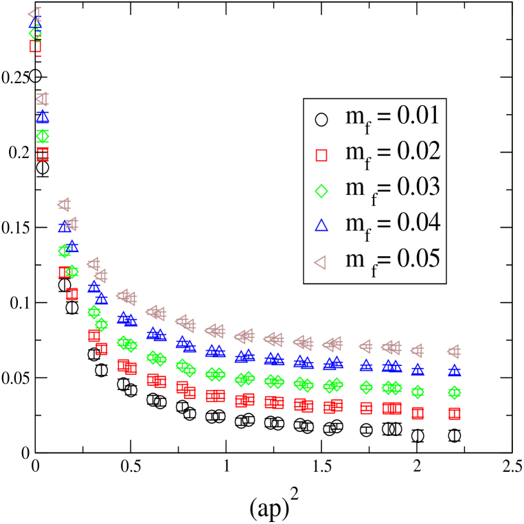
FIG. 1.: A plot of $\frac{1}{12}{\rm Tr}\left(S^{-1}_{latt}\right)$ versus $(ap)^{2}$ showing that for moderate values of $(ap)^{2}$ the effects of explicit chiral symmetry breaking are small.

FIG. 2.: The value of $\frac{1}{12}{\rm Tr}\left(S^{-1}\right)$ extrapolated to $m_{f}=0$ vs $(ap)^{2}$. For moderate $(ap)^{2}$ the extrapolated value is zero within errors, showing that the residual mass is small.

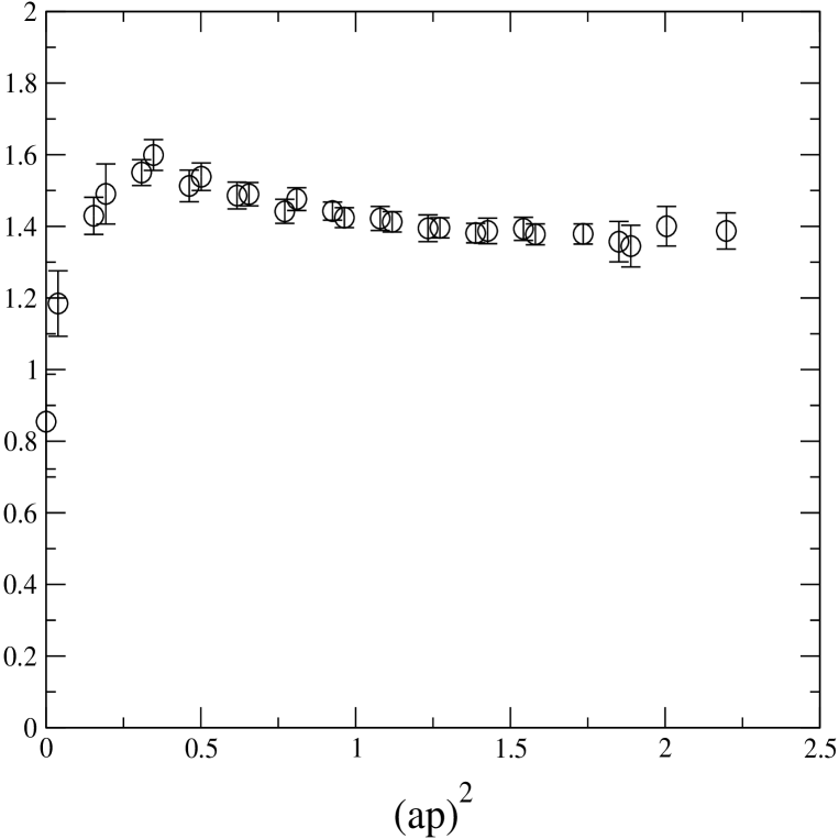
FIG. 3.: $Z_{m}Z_{q}$ calculated from the slope of $\frac{1}{12}{\rm Tr}\left(S^{-1}\right)$ versus $m_{f}$ plotted as a function of $(ap)^{2}$.

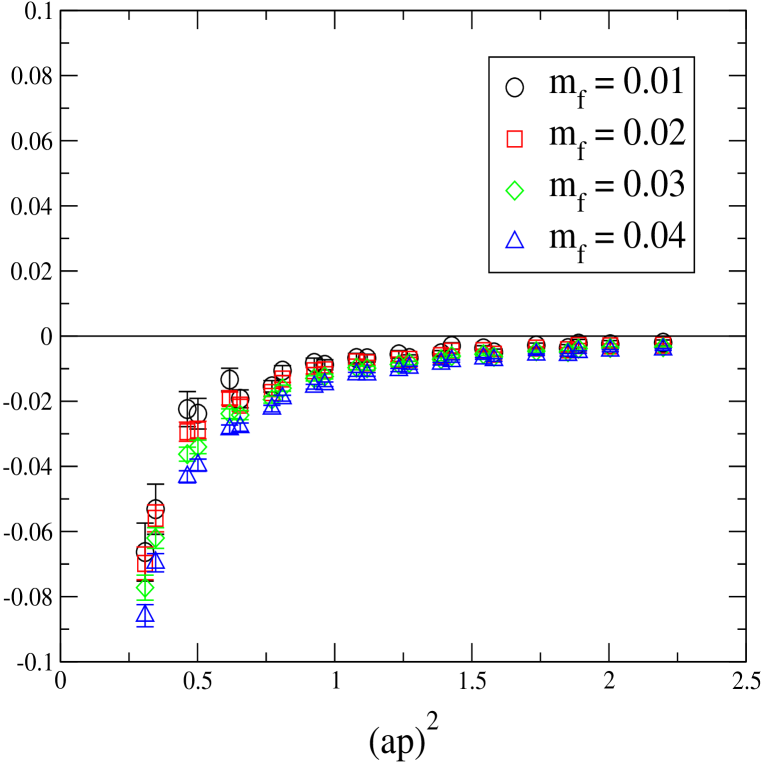
FIG. 4.: A plot of $\Lambda_{A}-\Lambda_{V}$ versus $(ap)^{2}$, showing that there is no significant difference between $Z_{A}$ and $Z_{V}$, even for moderate values of $(ap)^{2}$.

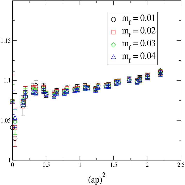
FIG. 5.: A graph of $\frac{1}{2}\left\{\Lambda_{A}+\Lambda_{V}\right\}$ versus $(ap)^{2}$, which up to lattice artifacts, gives $Z_{A}/Z_{q}$ and $Z_{V}/Z_{q}$.

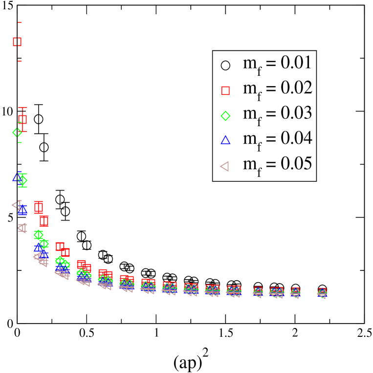
FIG. 6.: $\Lambda_{P}$ versus $(ap)^{2}$ for several values of $m_{f}$, showing that the $1/p^{2}$ pole is more pronounced for small $m_{f}$.

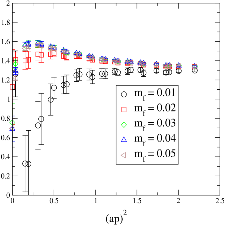
FIG. 7.: A plot of $\Lambda_{S,\mathrm{latt}}$ versus $(ap)^{2}$ for several masses. The mass pole can be clearly seen for small momenta and is attributable to zero-mode effects.

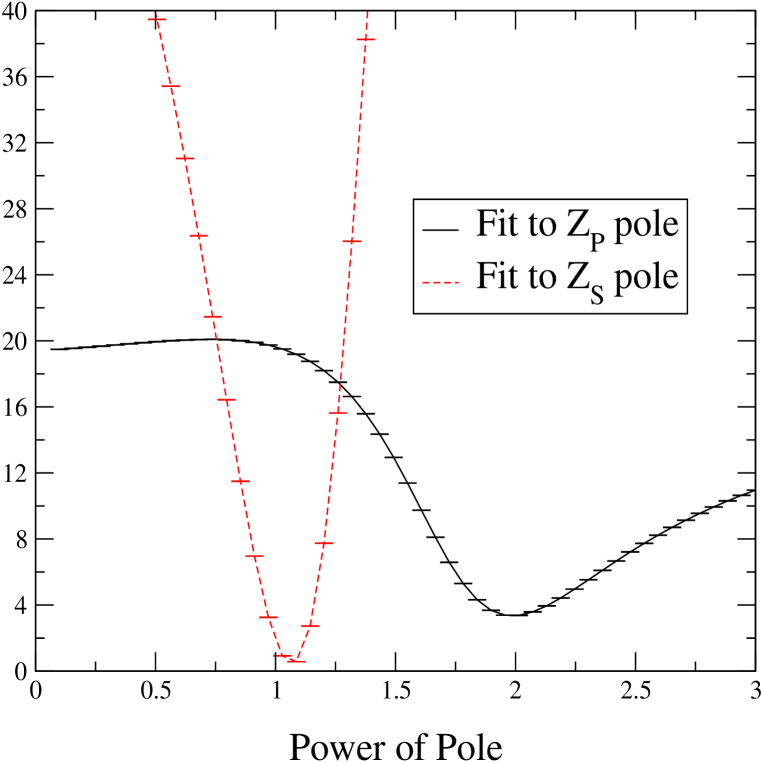
FIG. 8.: This figure displays the average $\chi^{2}$ per degree of freedom for the fits used to determine the power of the mass poles in $\Lambda_{S}$ and $\Lambda_{P}$, clearly showing their double and single poles, respectively.

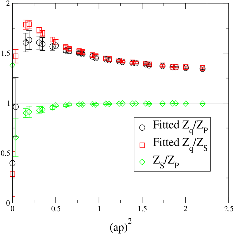
FIG. 9.: A comparison of $Z_{S}/Z_{q}$ and $Z_{P}/Z_{q}$ as extracted from $\Lambda_{S}$ and $\Lambda_{P}$ after pole subtraction.

FIG. 10.: The product $Z_{P}Z_{m}$ calculated by combining $Z_{P}/Z_{q}$ from pole subtraction with the trace of the inverse propagator. This product is clearly unity within errors.

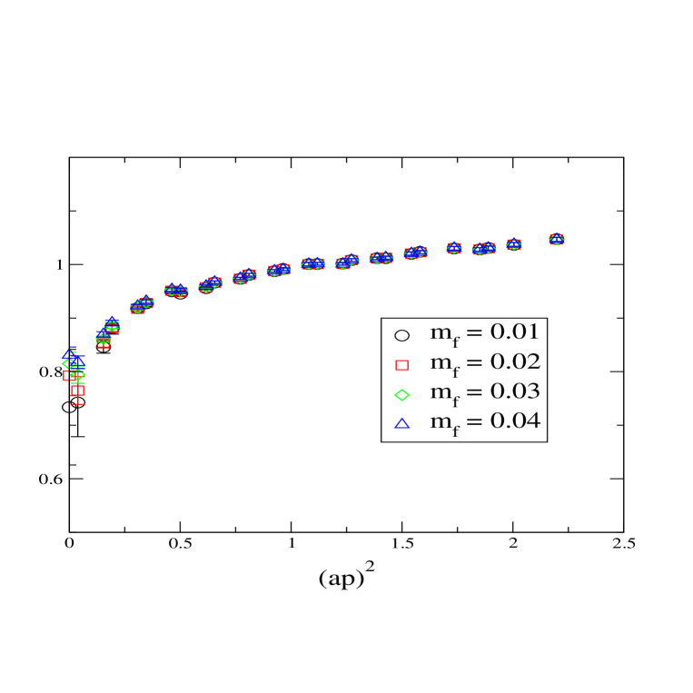
FIG. 11.: This is a graph of $\Lambda_{T}$ versus $(ap)^{2}$, from which $Z_{T}$ will be extracted in Section X.

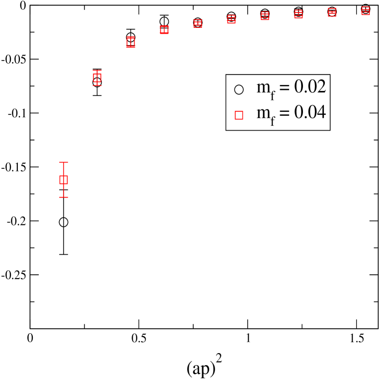
FIG. 12.: The difference between $Z_{q}$ as extracted from the conserved axial and vector currents.

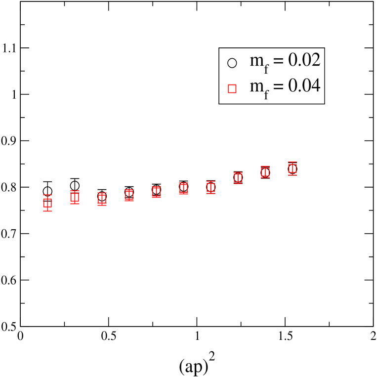
FIG. 13.: The average of $Z_{q}$ from the conserved axial and vector currents.

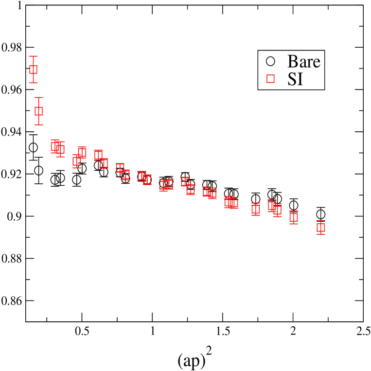
FIG. 14.: A plot showing the raw data for $1/\Lambda_{A}$ (labeled as “Bare”) and the value of $1/\Lambda_{A}$ divided by its predicted three loop perturbative running (labeled as “SI”), such that they coincide at $(ap)^{2}=1$, versus momentum. The slope of the latter versus $(ap)^{2}$ may be interpreted as an $\cal{O}$($a^{2}$) effect and is $\approx-0.02$.

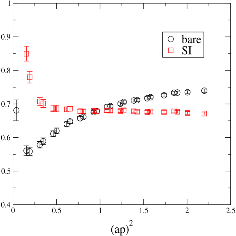
FIG. 15.: A plot showing the raw data for $1/\Lambda_{S}$ (labeled as “Bare”) and the value of $1/\Lambda_{S}$ divided by its predicted three loop perturbative running (labeled as “SI”), such that they coincide at $(ap)^{2}=1$, versus momentum. The slope of the latter versus $(ap)^{2}$ may be interpreted as an $\cal{O}$($a^{2}$) effect and is $\approx-0.003$.

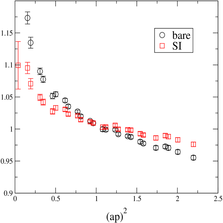
FIG. 16.: A plot showing the raw data for $1/\Lambda_{T}$ (labeled as “Bare”) and the value of $1/\Lambda_{T}$ divided by its predicted one loop perturbative running (labeled as “SI”), such that they coincide at $(ap)^{2}=1$, versus momentum. The slope of the latter versus $(ap)^{2}$ may be interpreted as an $\cal{O}$($a^{2}$) effect and is $\approx-0.02$.

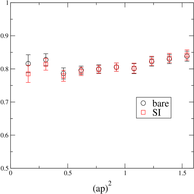
FIG. 17.: Bare and scale invariant (SI) versions of $Z_{q}$ determined from the conserved axial and vector currents.

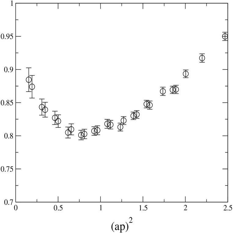
FIG. 18.: A scale invariant (SI) version of $Z_{q}$ determined from ${Z^{\prime}}_{q}$.

FIG. 19.: The scale invariant (SI) version of $Z_{q}$ determined from ${Z^{\prime}}_{q}$ but using $a\bar{p}_{\mu}$ instead of $ap_{\mu}$.

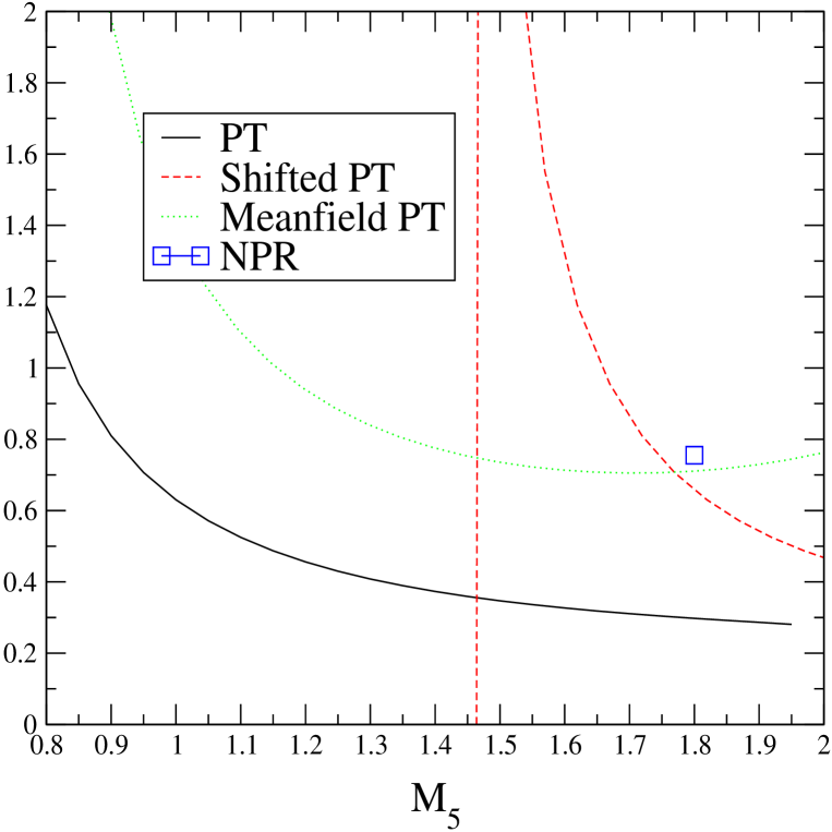
FIG. 20.: The renormalisation factor $Z_{A}^{\rm total}$ of Eq. 116 in the $\overline{\rm MS}$ scheme at $2~{}\mathrm{GeV}$ computed in naive perturbation theory, naive perturbation theory shifted by $(4-1/2\kappa_{c})$ as in Eq. 115 and mean field improved perturbation theory.

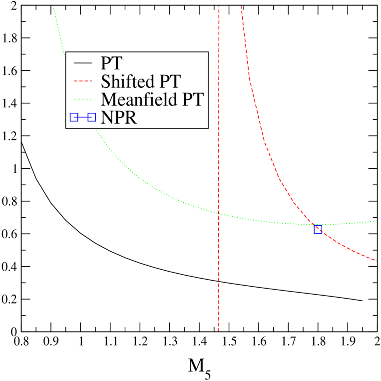
FIG. 21.: Same as Figure 20 but for $Z_{S}^{\rm total}$.

REFERENCES

- [1] S. J. Brodsky, G. P. Lepage, and P. B. Mackenzie, Phys. Rev. D28, 228 (1983).
- [2] G. P. Lepage and P. B. Mackenzie, Phys. Rev. D48, 2250 (1993), eprint hep-lat/9209022.
- [3] G. Martinelli, C. Pittori, C. T. Sachrajda, M. Testa, and A. Vladikas, Nucl. Phys. B445, 81 (1995), eprint hep-lat/9411010.
- [4] V. Gimenez, L. Giusti, F. Rapuano, and M. Talevi, Nucl. Phys. B531, 429 (1998), eprint hep-lat/9806006.
- [5] A. Donini, V. Gimenez, G. Martinelli, M. Talevi, and A. Vladikas, Eur. Phys. J. C10, 121 (1999), eprint hep-lat/9902030.
- [6] L. Giusti, V. Gimenez, F. Rapuano, M. Talevi, and A. Vladikas, Nucl. Phys. Proc. Suppl. 73, 210 (1999), eprint hep-lat/9809037.
- [7] D. Becirevic et al., Phys. Lett. B444, 401 (1998), eprint hep-lat/9807046.
- [8] S. Aoki et al. (JLQCD) The XVI International Symposium on Lattice Field Theory LATTICE 98, 14 - 18 Jul 1998, Boulder, Colorado, USA.
- [9] D. B. Kaplan, Nucl. Phys. Proc. Suppl. 30, 597 (1993).
- [10] Y. Shamir, Nucl. Phys. B406, 90 (1993), eprint hep-lat/9303005.
- [11] R. Narayanan and H. Neuberger, Nucl. Phys. B443, 305 (1995), eprint hep-th/9411108.
- [12] T. Blum et al. (2000), eprint hep-lat/0007038.
- [13] A. A. Khan et al. (CP-PACS) (2000), eprint hep-lat/0007014.
- [14] M. L. Paciello, S. Petrarca, B. Taglienti, and A. Vladikas, Phys. Lett. B341, 187 (1994), eprint hep-lat/9409012.
- [15] M. Gockeler et al., Nucl. Phys. B544, 699 (1999), eprint hep-lat/9807044.
- [16] V. Furman and Y. Shamir, Nucl. Phys. B439, 54 (1995), eprint hep-lat/9405004.
- [17] S. Aoki, T. Izubuchi, Y. Kuramashi, and Y. Taniguchi, Phys. Rev. D60, 114504 (1999), eprint hep-lat/9902008.
- [18] S. Aoki and Y. Taniguchi, Phys. Rev. D59, 094506 (1999), eprint hep-lat/9811007.
- [19] S. Aoki, T. Izubuchi, Y. Kuramashi, and Y. Taniguchi, Phys. Rev. D59, 094505 (1999), eprint hep-lat/9810020.
- [20] S. Aoki and Y. Taniguchi, Phys. Rev. D59, 054510 (1999), eprint hep-lat/9711004.
- [21] T. Blum, A. Soni, and M. Wingate, Phys. Rev. D60, 114507 (1999), eprint hep-lat/9902016.
- [22] T. Blum, Nucl. Phys. Proc. Suppl. 73, 167 (1999), eprint hep-lat/9810017.
- [23] M. Bochicchio, L. Maiani, G. Martinelli, G. C. Rossi, and M. Testa, Nucl. Phys. B262, 331 (1985).
- [24] D. Becirevic, V. Gimenez, V. Lubicz, and G. Martinelli (1999), eprint hep-lat/9909082.
- [25] H. D. Politzer, Nucl. Phys. B117, 397 (1976).
- [26] P. Pascual and E. de Rafael, Zeit. Phys. C12, 127 (1982).
- [27] E. Franco and V. Lubicz, Nucl. Phys. B531, 641 (1998), eprint hep-ph/9803491.
- [28] J.-R. Cudell, A. L. Yaouanc, and C. Pittori, Phys. Lett. B454, 105 (1999), eprint hep-lat/9810058.
- [29] T. Blum and S. Sasaki (2000), eprint hep-lat/0002019.
- [30] S. Capitani, M. Luscher, R. Sommer, and H. Wittig (ALPHA), Nucl. Phys. B544, 669 (1999), eprint hep-lat/9810063.
- [31] M. Guagnelli, R. Sommer, and H. Wittig (ALPHA), Nucl. Phys. B535, 389 (1998), eprint hep-lat/9806005.
- [32] K. G. Chetyrkin and A. Retey (1999), eprint hep-ph/9910332.
- [33] H. He and X. Ji, Phys. Rev. D52, 2960 (1995), eprint hep-ph/9412235.
- [34] S. Aoki, private communication .
- [35] A. J. Buras (1998), eprint hep-ph/9806471.