NTUA-2/01

QED₃ WITH DYNAMICAL FERMIONS IN AN EXTERNAL MAGNETIC FIELD

J. Alexandre${}^{a},$ K. Farakos^a, S.J. Hands^b, G. Koutsoumbas^a,
S.E. Morrison^b

^aDepartment of Physics, National Technical University of Athens,

Zografou Campus, 157 80 Athens, GREECE.

^bDepartment of Physics, University of Wales Swansea,

Singleton Park, Swansea SA2 8PP, U.K.

Abstract

In this paper, we present results of numerical lattice simulations of two-flavor QED in three space-time dimensions. First, we provide evidence that chiral symmetry is spontaneously broken in the chiral and continuum limit. Next we discuss the role of an external magnetic field $B$ on the dynamically generated fermion mass. We investigate the $B$-dependence of the condensate through calculations with dynamical fermions using the non-compact formulation of the gauge field, and compare the results with those of a comparable study using the quenched approximation.

1 Introduction

The intriguing phenomenon of high $T_{c}$ superconductivity has inspired several models, consisting mostly of elaborations of a doped version of the Hubbard model. The model presented in [1] claims the generation of superconductivity through a “mixed Chern-Simons term” without the need to introduce a local gauge symmetry breaking condensate. The model invokes the idea of electron substructure (spin-charge separation) considering the low-energy excitations of the system to be bosonic degrees of freedom called spinons and fermionic ones called holons. The role of the phonon interactions crucial to the formation of Cooper Pairs in BCS superconductors is now played by a “statistical” gauge field, which arises from the underlying dynamics of the holons hopping between lattice sites. More specifically, the model is based on a so-called $\tau_{3}$-U(1) interaction of the fermions with the gauge field.

An alternative form of the model has been proposed in [2]. The model is meant to represent the naïve continuum limit of the effective low-energy Hamiltonian of the large-$U$, doped Hubbard model. The action of the model reads:

$${\cal L}=-\frac{1}{4}(F_{\mu\nu})^{2}-\frac{1}{4}\mbox{tr}({\cal G}_{\mu\nu})^{2}+{\bar{\Psi}}D_{\mu}\gamma_{\mu}\Psi$$ (1)

where $D_{\mu}=\partial_{\mu}-ig_{1}A_{\mu}^{S}-ig_{2}\tau^{a}W_{a,\mu}-i\frac{e}{c}A_{\mu}^{ext}$, with $A_{\mu}^{S}$ the statistical U(1)_S gauge field, $W_{\mu}^{a}$ is the gauge potential of a local SU(2) group, and ${\cal G}^{a}_{\mu\nu}$ the corresponding field strength. The $\Psi$ fields are two-component spinors. The difference from the previous model lies in the fact that now the full gauge symmetry is $\mbox{U}(1)_{S}\otimes\mbox{SU}(2),$ where we have denoted by U(1)_S the abelian part of the symmetry. We call it a “statistical” gauge field since from the physical point of view it describes statistical properties of the model, such as the doping, and not real electromagnetism.

The strongly-coupled U(1)_S interaction promotes the spontaneous generation of a fermion – anti-fermion condensate resulting in a mass gap. Arguments based on energetics prohibit the generation of a parity-violating but SU(2) gauge invariant term [3], in favour of a parity-conserving condensate, which necessarily breaks the SU(2) group down to a $\tau_{3}$-U(1) sector [1]. The mass gap thus breaks the SU(2) part down to an abelian sub-group which is the analog of the $\tau_{3}$-U(1) in the model of [1]. The symmetry breaking pattern here follows the scheme: $\mbox{U(1)}_{S}\otimes\mbox{SU}(2)\rightarrow\mbox{U(1)}_{S}\otimes\mbox{U}(1)_{\tau_{3}}.$

In equation (1) we have also allowed for an additional U(1)_em coupling, which describes the coupling to an external electromagnetic field $A_{\mu}^{ext}$. Actual superconductivity is obtained upon coupling the system to such external electromagnetic potentials. We now discuss the superconducting consequences of the above dynamical breaking patterns of the SU(2) group. Upon the opening of a mass gap in the fermion (hole) spectrum, one obtains a non-trivial result for the following Feynman matrix element: ${\cal S}^{a}=\langle W^{a}_{\mu}|J_{\nu}|0\rangle,~{}a=1,2,3$, with $J_{\mu}={\bar{\Psi}}\gamma_{\mu}\Psi$ the fermion-number current. Due to the colour-group structure, only the massless $W^{3}_{\mu}$ gauge boson of the SU(2) group, corresponding to the $\tau_{3}$ generator in two-component notation, contributes to the matrix element. The non-trivial result for the matrix element ${\cal S}^{3}$ arises from an anomalous one-loop graph, and is given by [4, 1]:

$${\cal S}^{3}=\langle W^{3}_{\mu}|J_{\nu}|0\rangle=({\rm sgn}{M})\epsilon_{\mu\nu\rho}\frac{p_{\rho}}{\sqrt{p_{0}}}$$ (2)

where $M$ is the parity-conserving fermion mass generated dynamically by the U(1)_S group. As with other Adler-Bell-Jackiw anomalous graphs in gauge theories, the one-loop result (2) is exact and receives no contributions from higher loops [4]. This unconventional symmetry breaking (2), does not have a local order parameter [4, 1] since its formation is inhibited by strong phase fluctuations, thereby resembling the Kosterlitz-Thouless mode of symmetry breaking. The massless gauge boson $W_{\mu}^{3}$ of the unbroken $\tau_{3}$-U(1) subgroup of SU(2) is responsible for the appearance of a massless pole in the electric current-current correlator, which is the characteristic feature of any superconducting theory. As discussed in ref. [1], all the standard properties of a superconductor, such as the Meissner effect, infinite conductivity, flux quantization, the London limit of the action etc. are recovered in such a case. The field $W^{3}_{\mu}$, or rather its dual $\phi$ defined by $\partial_{\mu}\phi\equiv\epsilon_{\mu\nu\rho}\partial_{\nu}W^{3}_{\rho}$, can be identified with the Goldstone boson of the broken U(1)_em electromagnetic symmetry [1].

If an external magnetic field is coupled to the charged excitations about the superconducting state then new phenomena appear. In refs. [2, 5] it is argued that an external magnetic field in this (2+1)-dimensional system induces the opening of a second superconducting gap at the nodes of the $d$-wave gap, in agreement with recent experimental results on the behaviour of the thermal conductivity of high-temperature cuprates under the influence of strong external magnetic fields [6].

In this work we will study the phenomenon of the enhancement of the fermion condensate in the presence of an external magnetic field. In this respect it is not important to gauge the SU(2) group. We study QED₃, a model which in the continuum has a local U(1) symmetry and a global SU(2) symmetry. However, the lattice discretization we employ in order to perform non-perurbative calculations restricts the global symmetry to a U(1) “chiral” symmetry, which in turn is totally broken by the fermion – anti-fermion condensate $\langle\bar{\Psi}\Psi\rangle$. The question of whether this symmetry is spontaneously broken in QED₃, ie. whether $\langle\bar{\Psi}\Psi\rangle\not=0$ in the chiral limit bare fermion mass $m\to 0$ and the continuum (weak coupling) limit $g\to 0$, has been an important issue in non-perturbative field theory for many years. Initial studies based on Schwinger-Dyson (SD) studies using the photon propagator derived from the leading order $1/N_{f}$ expansion, where $N_{f}$ is the number of fermion flavors, suggested that for $N_{f}$ less than some critical value $N_{fc}$ the answer is positive [7], with $N_{fc}\simeq 3.2$. The model in the limit $N_{f}\to N_{fc}$ is supposed to undergo an infinite-order phase transition [8]. Other studies taking non-trivial vertex corrections into account predicted chiral symmetry breaking for arbitrary $N_{f}$ [9]. More recent studies which treat the vertex consistently in both numerator and denominator of the SD equations have found $N_{fc}<\infty$, with a value either in agreement with the original study [10], or slightly higher $N_{fc}\simeq 4.3$ [11]. Finally a recent argument based on a thermodynamic inequality has predicted $N_{fc}\leq{3\over 2}$ [12].

There have also been numerical attempts to resolve the issue via simulations of non-compact lattice QED₃. Once again, opinions have divided on whether $N_{fc}$ is finite and $\simeq 3$ [13], or whether chiral symmetry is broken for all $N_{f}$ [14]. The principal obstruction to a definitive answer has been large finite volume effects resulting from the presence of a massless photon in the spectrum, which prevent a reliable extrapolation to the thermodynamic limit. In this context it is also worth mentioning the three-dimensional Thirring model, which has a current-current interaction mediated in the UV limit by a propagator of identical form in the large-$N_{f}$ limit to that of QED₃; moreover chiral symmetry breaking for small $N_{f}$ is predicted by the same set of SD equations as those of QED₃ [15]. This time, however, the critical behaviour is governed by a UV-stable fixed point rather than an IR one, and numerical studies are more controlable, yielding values of $N_{fc}\simeq 5$ [16].

The rest of the paper is organised as follows. In section 2 we outline the formulation of continuum QED₃ in Euclidean metric, and identify its global symmetries. In section 3 we do the same for the lattice version of the model. We also review the formulation of a homogeneous background magnetic field $B$ in abelian lattice gauge theory. Our numerical results are presented in section 4. First for $B=0$, we attempt an extrapolation to both continuum and chiral limits, and observe evidence for a non-vanishing (though unexpectedly small) dimensionless chiral condensate, suggesting $N_{fc}>2$. We are also able to estimate the combination of lattice sizes and bare masses required for quantitative accuracy in further work. This work is described in section 4.1. In section 4.2 we turn to non-zero magnetic field $B$, and study the resulting enhancement of the condensate. This is the first lattice simulation of QED₃ with $B\not=0$ using dynamical fermions; the problem has previously been studied in the quenched approximation [17]. In particular we compare the behaviours of quenched versus dynamical fermions and calculate the condensate as a function of the magnetic field, and find different behaviours both in the strong and the weak field regimes, and in strong and weak U(1)_S coupling regimes. We conclude with a study of the dependence of the condensate in the strength of the statistical gauge interaction in the chiral limit, and uncover an important finite volume effect.

2 The model in the continuum and its symmetries

The three-dimensional continuum Lagrangian describing QED₃ is given (in Euclidean metric, which we use hereafter) by  [18, 2],

$${\cal L}=\frac{1}{4}F_{\mu\nu}^{2}+{\bar{\Psi}}_{i}D_{\mu}\gamma_{\mu}\Psi_{i}+m{\bar{\Psi}}_{i}\Psi_{i}$$ (3)

where $D_{\mu}=\partial_{\mu}-igA^{S}_{\mu}-ieA^{ext}_{\mu}$, and $F_{\mu\nu}$, ${\cal G}_{\mu\nu}$ are the corresponding field strengths for an abelian U(1)_S statistical gauge field $A^{S}_{\mu}$ and a background U(1)_em gauge field $A^{ext}_{\mu}$, respectively. The fermions $\Psi_{i}$, $i=1,\ldots,N_{f}$, are now four-component spinors. We note that $\Psi_{i}$ may be written in terms of the two-component spinors used in section 1 as

$$\Psi_{i}\equiv\left(\begin{array}[]{c}\Psi_{i1}\\ \Psi_{i2}\end{array}\right).$$ (4)

A convenient representation for the $\gamma_{\mu}$, $\mu=0,1,2$, matrices is the reducible $4\times 4$ representation of the Dirac algebra in three dimensions [7] (in Euclidean metric we choose hermitian Dirac matrices):

$$\gamma^{0}=\left(\matrix{\sigma_{3}&\phantom{-}{\bf 0}\cr{\bf 0}&-\sigma_{3}\cr}\right);\qquad\gamma^{1}=\left(\matrix{\sigma_{1}&\phantom{-}{\bf 0}\cr{\bf 0}&-\sigma_{1}\cr}\right);\qquad\gamma^{2}=\left(\matrix{\sigma_{2}&\phantom{-}{\bf 0}\cr{\bf 0}&-\sigma_{2}\cr}\right),$$ (5)

where $\sigma_{i}$ are $2\times 2$ Pauli matrices. Then the Lagrangian (3) decomposes into two parts, one for $\Psi_{i1}$ and one for $\Psi_{i2},$ which will be called “fermion species” in the sequel. The presence of an even number of fermion species allows us to define chiral symmetry and parity in three dimensions [7], which we discuss below. The bare mass $m$ term is parity conserving and has been added by hand in the Lagrangian (3). This term is generated dynamically anyway via the formation of the fermion condensate $\langle{\bar{\Psi}}\Psi\rangle$ by the strong U(1)_S coupling. Here we include such a term explicitly, since it is necessary from the technical point of view.

As is well known [7] there exist two $4\times 4$ matrices which anticommute with $\gamma_{\mu}$, $\mu=0,1,2$:

$$\gamma_{3}=\left(\matrix{{\bf 0}&{\bf 1}\cr{\bf 1}&{\bf 0}\cr}\right),\qquad\gamma_{5}=i\left(\matrix{\phantom{-}{\bf 0}&{\bf 1}\cr-{\bf 1}&{\bf 0}\cr}\right),$$ (6)

where the substructures are $2\times 2$ matrices. These are the generators of the ‘chiral’ symmetry for the massless fermion theory:

$$\Psi\rightarrow\exp(i\theta\gamma_{3})\Psi,\qquad\bar{\Psi}\rightarrow\bar{\Psi}\exp(i\theta\gamma_{3});$$ (7)

$$\Psi\rightarrow\exp(i\omega\gamma_{5})\Psi,\qquad\bar{\Psi}\rightarrow\bar{\Psi}\exp(i\omega\gamma_{5}).$$

Note that these transformations do not exist in the two-component representation of the three-dimensional Dirac algebra, and therefore the above symmetry is valid for theories with even numbers of fermion species only.

For later use we note that the Dirac algebra in $(2+1)$ dimensions satisfies the identities:

$$\gamma^{\mu}\gamma^{\nu}=-\delta^{\mu\nu}-\tau_{3}\epsilon^{\mu\nu\lambda}\gamma^{\lambda}\quad;\quad\tau_{3}\equiv i\gamma_{3}\gamma_{5}=\left(\matrix{{\bf 1}&\phantom{-}{\bf 0}\cr{\bf 0}&-{\bf 1}}\right)$$ (8)

$$\gamma^{\mu}\gamma^{\lambda}\gamma^{\mu}=\gamma^{\lambda}$$

$$\gamma^{\mu}\gamma^{0}\gamma^{\rho}\gamma^{\sigma}\gamma^{\mu}=-\delta^{\rho\sigma}\gamma^{0}-3\tau_{3}\epsilon^{\rho\sigma}$$

$$\gamma^{\mu}\gamma^{\rho}\gamma^{\sigma}\gamma^{\mu}=-3\delta^{\rho\sigma}-\tau_{3}\gamma^{0}\epsilon^{\rho\sigma}$$

$$\gamma^{\mu}\gamma^{\sigma}\gamma^{\rho}\gamma^{\tau}\gamma^{\mu}=-\delta^{\rho\sigma}\gamma^{\tau}-\delta^{\rho\tau}\gamma^{\sigma}+\delta^{\sigma\tau}\gamma^{\rho}$$

which are specific to three dimensions. Here the Greek letters are spacetime indices, and repetition implies summation.

Parity in this formalism is defined as the transformation:

$$P:~{}\Psi(x^{0},x^{1},x^{2}) \rightarrow -i\gamma_{3}\gamma_{1}\Psi(x^{0},-x^{1},x^{2});$$

$$\ \bar{\Psi}(x^{0},x^{1},x^{2}) \rightarrow \bar{\Psi}(x^{0},-x^{1},x^{2})i\gamma_{1}\gamma_{3},$$ (9)

and it is easy to see that the parity-invariant mass term $\bar{\Psi}\Psi$ corresponds to the species having masses with opposite signs  [7], whilst a parity-violating one $\bar{\Psi}\tau_{3}\Psi$ corresponds to masses of the same sign.

The set of generators

$${\cal G}=\{{\bf 1},\gamma_{3},\gamma_{5},\tau_{3}\}$$ (10)

form [18, 2] a global U(2) $\simeq$ SU(2)$\otimes$U(1) symmetry. To see this define $\tilde{\Psi}\equiv\bar{\Psi}\tau_{3}$. The U(2) symmetry is then

$$\Psi\rightarrow U\Psi\qquad\tilde{\Psi}\rightarrow\tilde{\Psi}U^{\dagger}\qquad U\in\mbox{U(2)}.$$ (11)

The identity matrix 1 generates the U(1) subgroup, while the other three form the SU(2) part of the group. The currents corresponding to the SU(2) transformations are:

$$J_{\mu}^{\Gamma}={\bar{\Psi}}\gamma_{\mu}\Gamma\Psi\qquad\Gamma=\gamma_{3},\gamma_{5},\tau_{3}$$ (12)

and are conserved in the absence of a fermionic mass term. It can be readily verified that the corresponding charges $Q_{\Gamma}\equiv\int d^{2}x\bar{\Psi}\gamma_{0}\Gamma\Psi$ lead to an SU(2) algebra [18]:

$$[Q_{3},Q_{5}]=2iQ_{\tau_{3}},\qquad[Q_{5},Q_{\tau_{3}}]=2iQ_{3},\qquad[Q_{\tau_{3}},Q_{3}]=2iQ_{5}.$$ (13)

In the presence of a mass term, these currents are not all conserved:

$$\partial^{\mu}J_{\mu}^{\Gamma}=2m{\bar{\Psi}}\Gamma\Psi,$$ (14)

for $\Gamma=\{\gamma_{3},\gamma_{5}\}$, while the currents corresponding to $\{{\bf 1},\tau_{3}\}$ are always conserved, even in the presence of a fermion mass. The situation parallels the treatment of the SU(2)$\otimes$SU(2) chiral symmetry breaking in low-energy QCD and the partial conservation of axial current (PCAC). The bilinears

$${\cal A}_{1}\equiv{\bar{\Psi}}\gamma_{3}\Psi,\qquad{\cal A}_{2}\equiv{\bar{\Psi}}\gamma_{5}\Psi,\qquad{\cal A}_{3}\equiv{\bar{\Psi}}\Psi$$ (15)

$$B_{1\mu}\equiv{\bar{\Psi}}\gamma_{\mu}\gamma_{3}\Psi,~{}B_{2\mu}\equiv{\bar{\Psi}}\gamma_{\mu}\gamma_{5}\Psi,~{}B_{3\mu}\equiv{\bar{\Psi}}\gamma_{\mu}\tau_{3}\Psi,~{}\mu=0,1,2$$

transform as triplets under SU(2). The SU(2) singlets are

$${\cal A}_{4}\equiv{\bar{\Psi}}\tau_{3}\Psi,\qquad B_{4,\mu}\equiv{\bar{\Psi}}\gamma_{\mu}\Psi$$ (16)

i.e. the singlets are the parity-violating mass term, and the four-component fermion current.

We now notice that in the case where the fermion condensate ${\cal A}_{3}$ is generated dynamically, energetics prohibit the generation of a parity-violating SU(2)-invariant term [3], and so a parity-conserving mass term necessarily breaks [2] the $U_{S}(1)\otimes$SU(2) group down to a $U_{S}(1)\otimes$U(1)${}_{\tau_{3}}$ group [1].

Finally, we note that were the global symmetries described here to be promoted to local ones, as they are in both the $\tau_{3}$-U(1) model of [1] and the $U_{S}(1)\otimes$SU(2) model of [2], then the measure of the Euclidean functional integral (i.e. the fermion determinant) would not be positive definite. Positivity of the theory defined by (3) follows because there exist matrices $\gamma_{3}$, $\gamma_{5}$ which anticommute with $D_{\mu}\gamma_{\mu}$; hence the imaginary eigenvalues of this antihermitian operator necessarily occur in conjugate pairs. This property no longer holds once, e.g., the U(1)${}_{\tau_{3}}$ symmetry is gauged. Thus this class of models suffer from a ‘sign problem’ in Euclidean metric, a feature shared with other potentially superconducting systems such as QCD at high baryon number density [19].

3 Lattice formulation

We now proceed with a description of the lattice formulation of the problem. The lattice action using staggered lattice fermion fields $\chi,\bar{\chi}$ is given by the formulæ below:

$$S=\frac{\beta_{G}}{2}\sum_{x,\mu<\nu}F_{\mu\nu}(x)F^{\mu\nu}(x)+\sum_{x,x^{\prime}}{\bar{\chi}}(x)Q(x,x^{\prime})\chi(x^{\prime})$$ (17)

$$F_{\mu\nu}(x)\equiv\alpha^{S}_{\mu}(x)+\alpha^{S}_{\nu}(x+\hat{\mu})-\alpha^{S}_{\mu}(x+\hat{\nu})-\alpha^{S}_{\nu}(x)$$

$$Q(x,x^{\prime})\equiv m\delta_{x,x^{\prime}}+\frac{1}{2}\sum_{\mu}\eta_{\mu}(x)[\delta_{x^{\prime},x+\hat{\mu}}U_{x\mu}V_{x\mu}-\delta_{x^{\prime},x-\hat{\mu}}U_{x-\hat{\mu},\mu}^{\dagger}V_{x-\hat{\mu},\mu}^{\dagger}].$$

The indices $x,~{}x^{\prime}$ consist of three integers $(x_{1},~{}x_{2},~{}x_{3})$ labelling the lattice sites, where the timelike direction is now considered as the third. Since the gauge action $F^{2}$ is unbounded from above, (17) defines the non-compact formulation of lattice QED. The $\eta_{\mu}(x)$ are Kawamoto-Smit phases $(-1)^{x_{1}+\cdots+x_{\mu-1}}$ designed to ensure relativistic covariance in the continuum limit. For the fermion fields antiperiodic boundary conditions are used in the timelike direction and periodic boundary conditions in the spatial directions. The phase factors in the fermion bilinear are defined by $U_{x\mu}\equiv\exp(i\alpha^{S}_{x\mu}),~{}~{}V_{x\mu}\equiv\exp(i\alpha^{ext}_{x\mu})$, where $\alpha^{S}_{x\mu}$ represents the statistical gauge potential and $\alpha^{ext}_{x\mu}$ the external electromagnetic potential. In terms of continuum quantities, $\alpha_{x\mu}^{S}=agA_{\mu}^{S}(x)$, the coupling $\beta_{G}\equiv\frac{1}{g^{2}a}$, and $\alpha_{x\mu}^{ext}=aeA_{\mu}^{ext}(x)$, where $a$ is the physical lattice spacing. The coupling $e$ to the external electromagnetic field is dimensionless.

The numerical results in this paper were obtained by simulating the action (17) using a standard Hybrid Monte Carlo (HMC) algorithm. The form of (17) permits an even-odd partitioning, which means that a single flavor of staggered fermion can be simulated. In the long wavelength limit, this can be shown to correspond to $N_{f}=2$ flavors of the four-component fermions $\Psi$ considered in section 2 [20]. Chiral condensation $\langle\bar{\Psi}\Psi\rangle\not=0$ would then result in a pattern $\mbox{U}(2N_{f})\rightarrow\mbox{U}(N_{f})\otimes\mbox{U}(N_{f})_{\tau_{3}}$. For non-zero lattice spacing $a$, however, the global symmetries for $m=0$ are only partially realised [16]. In this case the symmetry is

$$\bar{\chi}_{o}\rightarrow\bar{\chi}_{o}e^{i\alpha} \qquad\chi_{e}\rightarrow e^{-i\alpha}\chi_{e}$$

$$\bar{\chi}_{e}\rightarrow\bar{\chi}_{e}e^{i\beta} \qquad\chi_{o}\rightarrow e^{-i\beta}\chi_{o},$$ (18)

where $\chi_{o/e}$ denotes the field on odd (i.e. $\varepsilon(x)\equiv(-1)^{x_{1}+x_{2}+x_{3}}=-1$) and even sublattices respectively. Chiral symmetry breaking characterised by $\langle\bar{\chi}\chi\rangle\not=0$ now has the pattern $\mbox{U}(N)\otimes\mbox{U}(N)\rightarrow\mbox{U}(N)$ for $N$ flavors of staggered fermion.

We should now construct a lattice version of the homogeneous magnetic field. This has already been done before in [21] in connection with the abelian Higgs model. We follow a slightly different prescription, which we describe below [5], and which is closely related to a prescription for introducing a uniform topological charge density in two dimensions [22].

Since we would like to impose an external homogeneous magnetic field ${\bf B=\nabla\times\alpha}^{ext}$ in the (missing) $z$ direction, we choose the external gauge potential in such a way that the plaquettes in the $x_{1}x_{2}$ plane equal $B$, while all other plaquettes equal zero. One way in which this can be achieved is through the choice: $\alpha^{ext}_{3}(x_{1},x_{2},x_{3})=0,{\rm for~{}all}~{}x_{1},~{}x_{2},~{}x_{3},$ and

$$\alpha^{ext}_{1}(x_{1},x_{2},x_{3})=\cases{\phantom{(N+1}-\frac{B}{2}(x_{2}-1),&$x_{1}\neq N$;\cr-\frac{B}{2}(N+1)(x_{2}-1),&$x_{1}=N$:\cr}$$ (19)

$$\alpha^{ext}_{2}(x_{1},x_{2},x_{3})=\cases{\phantom{(N+2}+\frac{B}{2}(x_{1}-1),&$x_{2}\neq N$;\cr+\frac{B}{2}(N+1)(x_{1}-1),&$x_{2}=N$.\cr}$$

The lattice extent is assumed to be $N\times N$ in the $x_{1}x_{2}$ plane. It is trivial to check that all plaquettes starting at $(x_{1},x_{2},x_{3}),$ with the exception of the one starting at $(N,N,x_{3}),$ equal $B$. The latter plaquette equals $(1-N^{2})B=B-(N^{2}B).$ One may say that the flux is homogeneous over the entire $x_{1}x_{2}$ cross section of the lattice and equals $B.$ The additional flux of $-(N^{2}B)$ can be understood by the fact that the lattice is a torus, that is a closed surface, and the Maxwell equation ${\bf\nabla\cdot B}=0$ implies that the total magnetic flux through the $x_{1}x_{2}$ plane should vanish. This means that, if periodic boundary conditions are used for the gauge field, the total flux of any configuration should be zero, so the (positive, say) flux $B,$ penetrating the majority of the plaquettes will be accompanied by a compensating negative flux $-(N^{2}B)$ located on a single plaquette. This compensating flux should be “invisible”, that is it should have no observable physical effects. This is the case if the flux is an integer multiple of $2\pi:N^{2}B=n2\pi\Rightarrow B=n\frac{2\pi}{N^{2}},$ where $n$ is an integer. Thus we may say (disregarding the invisible flux) that the magnetic field is homogeneous over the entire cross section of the lattice. The integer $n$ may be chosen to lie in the interval $[0,\frac{N^{2}}{2}],$ since the model with integers between $\frac{N^{2}}{2}$ and $N^{2}$ is equivalent to that with integers taking on the values $N^{2}-n$. It follows that the magnetic field strength $B$ in lattice units lies between 0 and $\pi.$

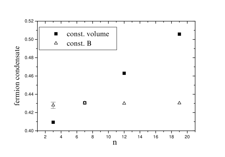
Figure 1: Fermion condensate versus $n$ for $m=0.1$ and $\beta_{G}=0.30.$ The solid squares are the results for a $12^{3}$ lattice. The triangles are data for which the volumes are different for each $n.$

The question of how to identify the continuum magnetic field strength $B_{phys}$ requires careful discussion. In the physical problem we wish to address the magnetic field is actually the $z$ component of a four-dimensional vector field, implying a relation $B=ea|\nabla\times{\bf A}^{ext}|=ea^{2}B_{phys},$ where $e$ is the electronic charge and is dimensionless. Therefore the combination $\beta_{G}^{2}B$ is dimensionless. The physical field may go to infinity letting the lattice spacing $a$ go to zero, while $B$ is kept constant.

On the lattice the magnetic field is determined by the number $n,$ but the allowed values of this number depend on the lattice size $N.$ On the contrary, the parameter $B$ does not depend much on the details of the discretization, so it is natural to choose it as the most natural lattice unit for the magnetic field. In figure 1 we show the fermion condensate versus $n.$ The solid squares represent the condensate for a $12^{3}$ lattice for several values of $n.$ We observe that the condensate increases substantially with $n,$ since different $n$ yield different values for $B.$ The triangles represent data produced by taking each $n$ with an appropriate volume, such that $B$ remains almost constant; the resulting $(n,N^{3})$ pairs turn out to be: $(3,8^{3}),~{}(7,12^{3}),~{}(12,16^{3}),~{}(19,20^{3}).$ It is obvious that in this way we get essentially the same condensate for all $n.$

An important remark is that the magnetic field should not be allowed to grow too big in lattice units, since then the perturbative expansion of the expansions $\exp(i\alpha^{ext}_{x\mu})$ would yield significant $B^{2},~{}B^{3},\dots$ contributions with the accompanying vertices, in addition to the desired terms which are linear in $B.$ A trivial estimate of the critical field strength is obtained from the demand that the cyclotron radius corresponding to a given magnetic field should not be less than (say) two lattice spacings. This calculation yields $B<\frac{\pi}{8}.$ Of course the above limitations apply strictly only to the case where the statistical gauge field has been turned off; in the interacting case, one does not really know whether there exists a critical magnetic field after which discretization effects are important. With this remark in mind, we depict in the figures of the following sections the results for the whole range of the magnetic field, from 0 to $\pi.$

4 Simulation results

4.1 $B=0$

It is instructive to begin by studying the case $B=0$. We have performed simulations on $12^{3}$ and $16^{3}$ lattices for a range of gauge couplings $\beta_{G}\in[0.5,0.8]$ and bare fermion masses $m\in[0.01,0.05]$. For each parameter set we accumulated $O(2000)$ HMC trajectories of mean length 0.9, with timesteps ranging from $d\tau=0.05$ on $12^{3}$ with $m=0.05$ to $d\tau=0.025$ on $16^{3}$ with $m=0.01$. The chiral condensate $\langle\bar{\chi}\chi\rangle$ was estimated by stochastic means using 10 noise vectors every two trajectories. Our data is shown in Fig. 3. It is clear that finite volume effects are significant; this can be attributed to the presence of a massless particle, the photon, in the spectrum of the theory. Large finite volume effects are the main source of difficulty in numerical studies of QED₃ [13, 14]. We will not attempt to extrapolate to the thermodynamic limit, but instead focus on the $16^{3}$ results.

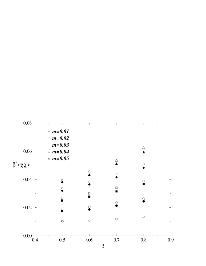
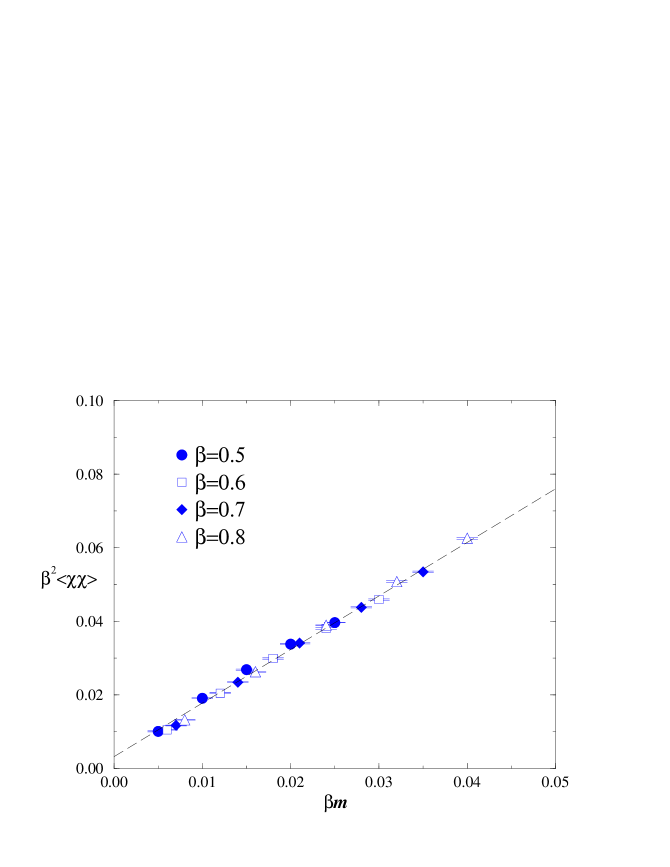
Figure 2: $\beta_{G}^{2}\langle\bar{\chi}\chi\rangle$ vs. $\beta_{G}$ on $12^{3}$ (filled) and $16^{3}$ (open) lattices.

Figure 3: $\beta_{G}^{2}\langle\bar{\chi}\chi\rangle$ vs. $\beta_{G}m$ from a $16^{3}$ lattice.

Note that in Fig. 3 we have chosen to plot the dimensionless combination $\beta_{G}^{2}\langle\bar{\chi}\chi\rangle$. Since QED₃ is an asymptotically-free theory (recall $g$ has positive mass dimension), its continuum limit lies in the limit $\beta_{G}\to\infty$. To see whether lattice data taken with $a\not=0$ are characteristic of the continuum limit, it is helpful to plot dimensionless quantities against each other; results from different $\beta_{G}$ should fall on a universal curve if continuum physics is being probed. We show a plot of $\beta_{G}^{2}\langle\bar{\chi}\chi\rangle$ vs. $\beta_{G}m$ in Fig. 3. The data do indeed fall approximately on a straight line, the main departures being at the strongest coupling $\beta_{G}=0.5$, and the smallest mass $m=0.01$, which might plausibly be attributed respectively to lattice artifacts and finite volume effects. If we exclude these points, a straight line fit of the form $\beta_{G}^{2}\langle\bar{\chi}\chi\rangle=0.00327(15)+1.454(6)\beta_{G}m$ is achieved (if the equivalent points from $12^{3}$ are used, the fitted line is $0.00140(16)+1.436\beta_{G}m$).

The main result of these fits is that the value of $\beta_{G}^{2}\langle\bar{\chi}\chi\rangle$ extrapolated to the chiral limit is unusually small, but significantly different from zero. If the linear form really does characterise the continuum limit, then this result is robust even on our admittedly small volumes. The implication is that chiral symmetry is broken in the the IR limit for $N_{f}=2$ flavors of fermion in QED₃, and hence $N_{fc}>2$. This is consistent with the findings of most studies using the gap equation, but contradicts a recent bound $N_{fc}\leq\frac{3}{2}$ derived by counting massless degrees of freedom via the absolute value of the thermodynamic free energy $f$ in both IR and UV limits [12], and demanding

$$f_{IR}\leq f_{UV}.$$ (20)

A possible resolution follows from the discussion below eqn. (18); the global symmetry of the lattice model is smaller than that of continuum QED₃, resulting in a smaller number of Goldstone bosons in the chirally broken phase. For $N$ flavors of staggered fermion, there are $8N=4N_{f}$ fermionic degrees of freedom in the UV limit, and $N^{2}$ Goldstone boson degrees of freedom in the IR. Following the argument of [12], we arrive at the bound $N_{c}\leq 6$ for the lattice model, which clearly is not threatened by our results. To substantiate this it will be necessary to show that the strongly-coupled dynamics of the IR limit is governed by the symmetries of the lattice model rather than the continuum one [16].

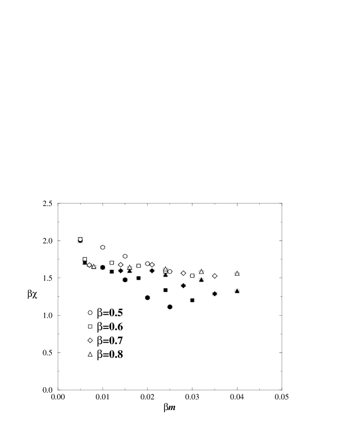
Figure 4: $\beta_{G}\chi_{l}$ (filled) and $\beta_{G}\chi_{t}$ (open) vs. $\beta_{G}m$ from a $16^{3}$ lattice.

Next we discuss longitudinal and transverse susceptibilities, defined respectively as the integrated propagators in scalar and pseudoscalar meson channels:

$$\chi_{l}=\sum_{x}\langle\bar{\chi}\chi(0)\bar{\chi}\chi(x)\rangle;\qquad\chi_{t}=\sum_{x}\langle\bar{\chi}\varepsilon\chi(0)\bar{\chi}\varepsilon\chi(x)\rangle.$$ (21)

The longitudinal susceptibility $\chi_{l}$ has contributions from diagrams with both connected and disconnected fermion lines [16]; we find that the connected contribution is overwhelmingly dominant throughout our parameter space. The transverse susceptibility is most conveniently calculated via the axial Ward identity $\chi_{t}=\langle\bar{\chi}\chi\rangle/m$. The results are plotted using dimensionless quantities in Fig. 4. We see that the evidence for universal scaling behaviour in the dimensionless plots is much less convincing, particularly for $\chi_{l}$ for $\beta_{G}m\geq 0.01$. At the smallest $m$ values the two susceptibilities even coincide within errors, suggesting that chiral symmetry is unbroken. This is probably because the data from different $\beta_{G}$ are taken on different physical volumes, and two-point functions (21) are prone to finite volume effects, particularly since a Goldstone boson is anticipated in the transverse channel as $m\to 0$. We can observe a tendency for $\chi_{t}$ to increase as this limit is approached. Bearing in mind the linear fit to the data of Fig. 3, however, we might expect to have to go to mass values as small as $\beta_{G}m\approx 0.002$ before the divergence in $\chi_{t}$ due to a Goldstone pole becomes dominant. Results in this regime in both continuum and thermodynamic limits will be required for universal statements about the nature of the IR limit to become feasible.

4.2 $B\not=0$

In this subsection we present the behaviour of fermionic matter under the combined action of the external magnetic field and the quantum gauge field. Before going on with the specific features of these results, let us remark that to facilitate comparison with the analytic results [5] we measured the magnetic field in units of its maximal value: thus we used the parameter $b\in[0,1]$ defined by $b\equiv B/B_{max}=B/\pi$.

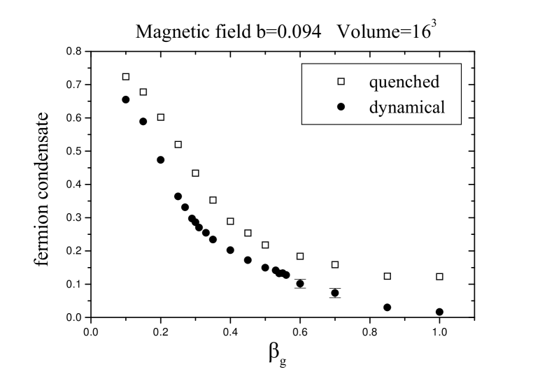
Figure 5: Fermion condensate versus $\beta_{G}$ for quenched and dynamical fermions at b=0.094.

A comparison of the dynamical and the quenched results is made in figure 5. A $16^{3}$ lattice has been used for the calculation, while the external magnetic field has been set to $b=0.094,$ a typical value. Measurements have been done at several values of the bare mass $m$ and what we show in figure 5 is the extrapolation to the $m\to 0$ limit. The method of extrapolation will be explained in more detail in the discussion of figure 10 below. The volume dependence is not very big in the quenched case [17]. We observe that the values for the condensate in the quenched case are rather large for the relatively large value $\beta_{G}=1.0$ for the gauge coupling. In principle the condensate should vanish for $\beta_{G}\rightarrow\infty,$ since the system moves to the “free” case, and the lattice volume is fixed. Presumably, even the quenched condensate will vanish, but the figure suggests that this will require a much bigger value of $\beta_{G}.$

The fact that the full condensate for dynamical fermions is smaller than the corresponding quantity for quenched fermions has presumably to do with Pauli repulsion, which has clearly an effect in the dynamical fermion case.

The next set consists of measurements of the fermion condensate versus the magnetic field for a $16^{3}$ lattice at a fixed, strong coupling for the statistical gauge field $(\beta_{G}=0.10)$, for five values of the bare mass (figure 7).

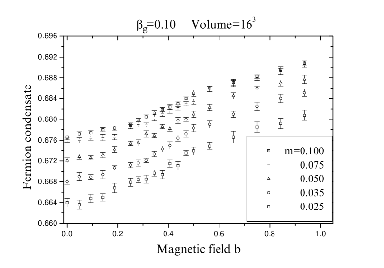
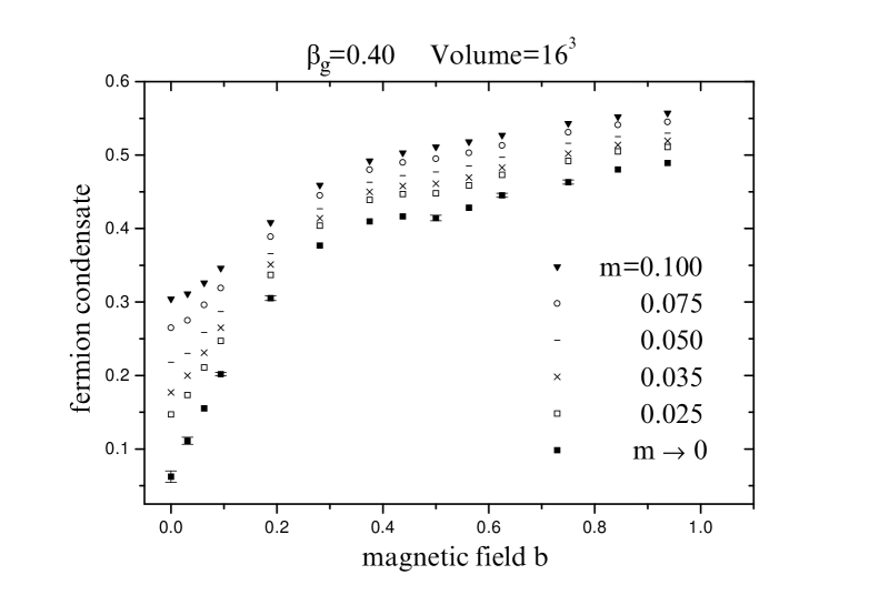
Figure 6: Fermion condensate at strong coupling versus the magnetic field for various bare masses.

Figure 7: Mass dependence for intermediate $\beta_{G}.$

For all five masses the plot consists of two parts with different behaviour. For relatively small $b$ we find a dependence of the condensate on the external magnetic field which is nearly linear. For relatively big magnetic fields we find points that have a qualitatively different behaviour. The two regions merge smoothly. The “linear” part of the graph appears to extend in a wider interval of $b$ for decreasing mass. It should be stressed that the mass dependence of the condensate is in sharp disagreement with the corresponding result in [17], where quenched fermions have been used. The condensate increases with the bare mass for all values of the magnetic field strength, whereas in the quenched case it was decreasing. The $m\to 0$ extrapolation of the results lies probably under the lowest curve, however at this stage our statistics are not good enough to get reliable numbers for the limiting values of the condensate.

It is interesting to know what happens as one moves towards weaker couplings. Based on the results of the quenched case [17] we expect that the almost linear part referred to previously would be restricted to very small magnetic fields and eventually disappear. In figure 7 we show the results for the coupling $\beta_{G}=0.40.$ The linear part has indeed been restricted to the region $b<0.2.$ Moreover, we show the bare mass dependence along with the $m\to 0$ limit of the condensate versus $b.$ It is interesting to note that the data for each particular mass give a monotonic dependence, while the $m\to 0$ limit starts having a local minimum at $b\simeq 0.5$, which is characteristic of the free case, ie. with the statistical gauge field turned off, to which we now turn.

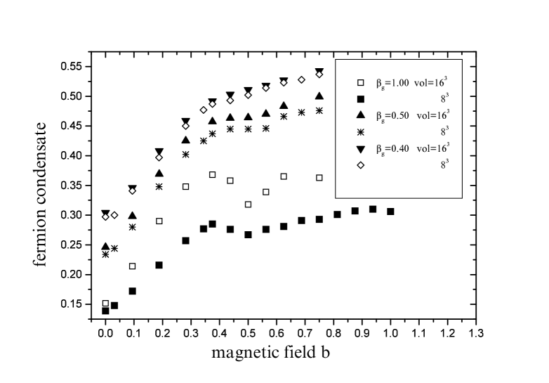
Figure 8: Approach to the free case in the limit of large $\beta_{G}$ and a fixed fermion mass $m=0.100.$

The free case was studied in [5], where it was found that for big enough $b$ the condensate stopped being monotonic and started showing local maxima and minima. It developed the first local minimum at $b=0.5$ and then it had a succession of maxima and minima, up to $b=1.$ Moreover, there was a spectacular volume dependence. One expects, of course, that this free case will be reached for big enough $\beta_{G}.$

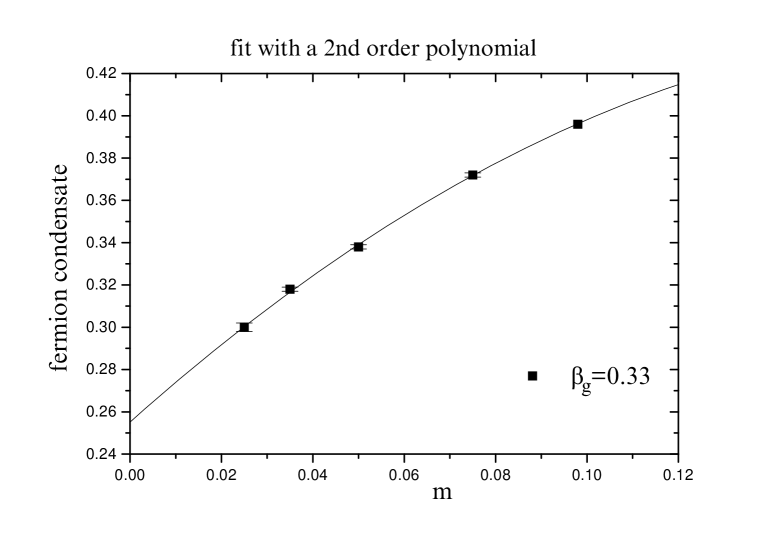
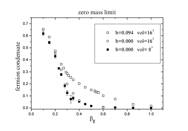
Figure 9: Extrapolation to the zero mass limit for $\beta_{G}=0.33$ and b=0.094.

Figure 10: $\beta_{G}$–dependence of the condensate for two values of the magnetic field: $b=0$ and $b=0.094.$

We have seen this kind of approach to the free model in the quenched fermion case [17]. In figure 8 we show the results for $\beta_{G}=0.40$, 0.50 and 1.00 for two volumes, $8^{3}$ and $16^{3}.$ The coupling $\beta_{G}=0.50$ is the point where the curve shows the first sign of non-monotonous behaviour. At $\beta_{G}=1.00$ the successive maxima and minima are clear. These features are shared with the quenched case. However, in the quenched calculation the volume dependence was not visible, while in this case, one can see the volume dependence at all values of the parameters. In the intermediate coupling regime ($\beta_{G}=0.40$ and $\beta_{G}=0.50$) the volume dependence, although clear, is rather small; at $\beta_{G}=1.00$ the volume dependence is comparable with that of the free case. In view of this behaviour we may be confident that, at this large $\beta_{G},$ the limit of switching the gauge field off can be reached if one uses dynamical fermions, in contradistinction with the quenched calculation [17]. One should remark that in the free case the role of the bare mass is very important, since it is eventually the only source of mass generation. This is at the root of the large volume dependence showing up in the free case: at fixed volume the condensate goes over to zero for vanishing bare mass. In the quenched interacting model, though, the interaction with the gauge field generates a dynamical mass, independently from the value of the bare mass. The volume dependence is thus small, permitting a smooth transition to the thermodynamic, as well as to the massless, limit [23]. In the present case with the dynamical fermions, the dynamically generated mass is suppressed, presumably due to the Pauli repulsion which is in full operation here, so the value of $\beta_{G}$ for which we have the transition to the free case is rather small compared to the quenched calculation.

Now we are going to explain in some detail the procedure we followed to obtain the $m\to 0$ limit. The simulations have been done at non-zero values of the bare mass; the massless limit has been taken by extrapolating the results for several bare masses to the limit $m\to 0.$ Figure 10 shows the process of this extrapolation for $\beta_{G}=0.33$ and the external magnetic field $b$ set equal to 0.094. The general behaviour is similar to that of the quenched case, in the sense that in the strong coupling region this curve is an almost straight line with a small slope and in the weak gauge coupling a second order polynomial proves necessary to perform the fit. At strong coupling the mass dependence is not very big, because it is the strong gauge coupling which dominates in the formation of the condensate. The error bars appear to be smaller here as compared to the gauge couplings of similar magnitude in the quenched case [17].

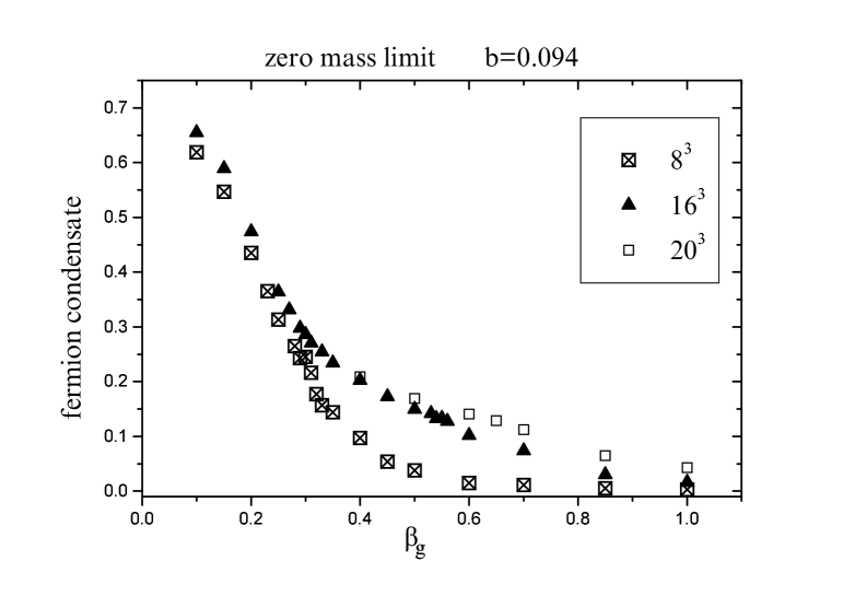
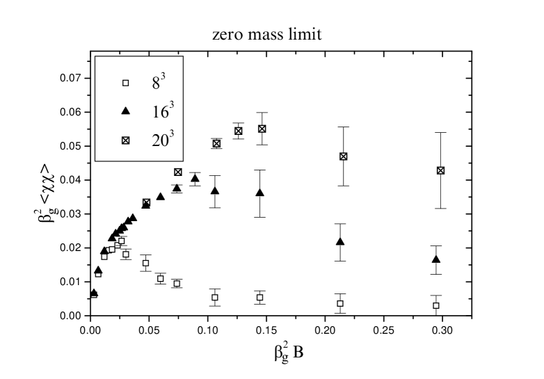
Figure 11: Volume dependence and finite size effects for dynamical fermions in the zero mass limit.

Figure 12: Finite size effects for dynamical fermions in the zero mass limit using dimensionless variables.

Figure 10 contains the zero mass limit of the condensate (obtained through the procedure illustrated in figure 10) versus $\beta_{G}$ for $b=0$ and $b=0.094.$ In the former case the bulk of the results come from $8^{3}$ lattice, however we also present some results from $16^{3},$ just to get some feeling about the volume dependence. We observe that in the strong coupling region the $b$-dependence of the condensate is rather weak; on the contrary, at weak coupling, the external field is the main generator of the condensate, and we find an increasingly big $b$-dependence as we move to large $\beta_{G}.$ In particular for zero external field the result is very small for $\beta_{G}>0.5,$ while the external field at these values of the gauge coupling still generates a relatively big condensate.

The volume dependence of the condensate at $b=0.094$ for a wide range of $\beta_{G}$ is shown in figure 12. For the smallest volume $8^{3}$ the data exhibit a rather big cusp at $\beta_{G}\simeq 0.30.$ For the two bigger volumes $16^{3}$ and $20^{3}$ the slopes are discontinuous at $\beta_{G}\simeq 0.53$ and $\beta_{G}\simeq 0.60$ respectively, but the discontinuity is smaller. It appears to be a finite size effect, possibly a shadow of the deconfining transition for each volume at weak coupling. The dynamically generated mass is smaller for the model with dynamical fermions as compared to the quenched model for the same value of the gauge coupling; so the finite size effects become more manifest.

In figure 12 we rescale the axes of figure 12, such that we get dimensionless units. In particular, we use $\beta_{G}^{2}B\to eB_{phys}/g^{4}$ for the $x$ axis and $\beta_{G}^{2}\langle{\bar{\chi}}\chi\rangle\to\langle{\bar{\chi}}\chi\rangle|_{phys}/g^{4}$ for the $y$ axis. What was a cusp in figure 12 has been transformed into a maximum in dimensionless units. The condensate starts increasing with the external magnetic field, now that it is properly rescaled, but finally the finite size effects take over and the condensate starts decreasing. The value of the magnetic field where this happens increases with the lattice volume and presumably tends to infinity in the thermodynamic limit.

5 Summary

After reviewing and contrasting the formulation and global symmetries of QED₃ in continuum field theory and on the lattice, we have presented numerical results from a Monte Carlo simulation study using dynamical fermions. For $B=0$ our calculations used the largest system sizes studied to date to our knowledge; for $B\not=0$ this is the first such study. Our principal results are as follows:

• For $B=0$ we have evidence, on the assumption of a linear scaling relation, for spontaneously broken chiral symmetry in the chiral and thermodynamic limits for $N_{f}=2$ flavors of four-component fermion. The condensate $\langle\bar{\chi}\chi\rangle$ has an unusually small value, $O(10^{-3})$ in natural units, which perhaps explains why this issue has proved a “difficult” problem in non-perturbative field theory. Our results should inform future studies on the system sizes needed in order for universal statements about the continuum theory to be possible.

• We have studied the response of the condensate to an external magnetic field in the regimes of strong, intermediate and weak U(1)_S coupling. In all cases $\langle\bar{\chi}\chi\rangle$ is smaller than that found in comparable quenched simulations. As in the quenched case, for strong and intermediate coupling regimes the condensate increases monotonically with $B$, but the behaviour becomes non-monotonic at weaker coupling. In the weak coupling limit contact with the behaviour of free fermions including volume dependence is recovered, in contrast with the quenched model.

• We have used our results in the chiral limit to make a plot of condensate against external field in dimensionless units (Fig. 12), which enables a significant finite volume effect to be identified. The condensate increases as a smooth monotonic function of $\beta_{G}^{2}B$ with negative curvature. Future studies with different values of the lattice magnetic field parameter $b$ will help to establish whether this behaviour is universal, and hence characterises the continuum limit. We note that in the Schwinger-Dyson approach [24] the regime of small magnetic fields could not be efficiently treated, while this is feasible with the Monte Carlo approach.

References

- [1] N. Dorey and N.E. Mavromatos, Phys. Lett. 250B (1990) 907; Nucl. Phys. B386 (1992) 614; For a comprehensive review of this approach see: N.E. Mavromatos, Nucl. Phys. B (Proc. Suppl.) C33 (1993) 145.
- [2] K. Farakos and N.E. Mavromatos, Phys. Rev. B57 (1998) 3017; Int. J. Mod. Phys. B12 (1998) 809.
- [3] C. Vafa and E. Witten, Comm. Math. Phys. 95 (1984) 257.
- [4] A. Kovner and B. Rosenstein, Phys. Rev. B42 (1990) 4748.
- [5] K. Farakos, G. Koutsoumbas and N.E. Mavromatos, Phys. Lett. B431 (1998) 147.
- [6] K. Krishana et al, Science 277 (1997) 83.
-
[7]
R.D. Pisarski, Phys. Rev. D29 (1984) 2423;
T.W. Appelquist, M. Bowick, D. Karabali and L. C. R. Wijewardhana, Phys. Rev. D33 (1986) 3704;
T.W. Appelquist, D. Nash and L.C.R. Wijewardhana, Phys. Rev. Lett. 60 (1988) 2575. -
[8]
V.A. Miranskii and K. Yamawaki, Phys. Rev. D55 (1997)
5051;
V.P. Gusynin, V.A. Miranskii and A.V. Shpagin, Phys. Rev. D58 (1998) 085023. -
[9]
M.R. Pennington and S.R. Webb, Brookhaven preprint
BNL-40886;
M.R. Pennington and D. Walsh, Phys. Lett. B253 (1991) 246. - [10] P. Maris, Phys. Rev. D54 (1996) 4049.
-
[11]
D. Nash, Phys. Rev. Lett. 62 (1989) 3024;
K.-I. Kondo, T. Ebihara, T. Iizuka and E. Tanaka, Nucl. Phys. B434 (1995) 85;
I.J.R. Aitchison, N.E. Mavromatos and D.O. McNeill, Phys. Lett. B402 (1997) 154. - [12] T.W. Appelquist, A.G. Cohen and M. Schmaltz, Phys. Rev. D60 (1999) 045003.
-
[13]
E. Dagotto, A. Kocić and J.B. Kogut, Phys. Rev. Lett. 62 (1989) 1083;
Nucl. Phys. B334 (1990) 279;
J.B. Kogut and J.-F. Lagaë, Nucl. Phys. B(Proc. Suppl.)30 (1993) 737. - [14] V. Azcoiti and X.-Q. Luo, Mod. Phys. Lett. A8 (1993) 3635.
-
[15]
T. Itoh, Y. Kim, M. Sugiura and K. Yamawaki,
Prog. Theor. Phys. 93 (1995) 417;
M. Sugiura, Prog. Theor. Phys. 97 (1997) 311. -
[16]
L. Del Debbio, S.J. Hands and J.C. Mehegan, Nucl. Phys.
B502 (1997) 269;
L. Del Debbio and S.J. Hands, Nucl. Phys. B552 (1999) 339;
S.J. Hands and B. Lucini, Phys. Lett. B461 (1999) 263. - [17] K. Farakos, G. Koutsoumbas, N.E. Mavromatos and A. Momen, Phys. Rev. D61 (2000) 45005.
-
[18]
K. Farakos, G. Koutsoumbas and
G. Zoupanos, Phys. Lett. B249 (1990) 101;
K. Farakos and G. Koutsoumbas, Phys.Lett. B178 (1986) 260. - [19] eg. S.J. Hands and S.E Morrison, in Understanding Deconfinement in QCD, ECT∗ Trento (1999) (World Scientific eds. D. Blaschke et al.) p. 31 hep-lat/9905021.
- [20] C.J. Burden and A.N. Burkitt, Europhys. Lett. 3 (1987) 545.
- [21] P. Damgaard and U.M. Heller, Nucl. Phys. B309 (1988) 625.
- [22] J. Smit and J.C. Vink, Nucl. Phys. B286 (1987) 485.
- [23] S.J. Hands and J.B. Kogut, Nucl. Phys. B335 (1990) 455.
- [24] J. Alexandre, K. Farakos and G. Koutsoumbas, Phys. Rev. D62 (2000) 105017.