Light Hadron Weak Matrix Elements CPT-2000/P.4091
LAPTH-Conf-821/00

Abstract

I review this year’s developments in the study of weak matrix elements of light hadrons on the lattice, with emphasis on $K^{0}{-}\bar{K}^{0}$ mixing and $K\to\pi\pi$ decays.

1 Introduction

Weak processes involving light hadrons in general, and kaons in particular, have contributed significantly to our understanding of fundamental interactions over the years. Most recently, the measurement of a non-vanishing $\mathrm{Re}\;\epsilon^{\prime}/\epsilon$ in $K\to\pi\pi$ decays by KTeV [2] and NA48 [3] has provided unambiguous evidence for direct CP violation.

In constraining the Standard Model (SM), the physics of kaons is complementary to that of $B$ mesons. This is clearly visible in Figure 1, where the types of constraints imposed by weak processes involving either of these particles are displayed. Kaons provide an important constraint on the summit of the unitarity triangle through the measurement of $\epsilon$, the parameter which quantifies indirect CP violation in $K\to\pi\pi$ decays. This constraint requires a description of non-perturbative effects in $K^{0}{-}\bar{K}^{0}$ mixing, parametrized by $B_{K}$. Lattice results for this quantity are commonly used in unitarity triangle fits. There are two new results this year for $B_{K}$, obtained with domain-wall fermions, by the CP-PACS [4] and RBC [5] collaborations.

Rare kaon decays and other FCNC kaon processes also provide good probes of physics beyond the SM. Here too the lattice is contributing. Donini et al. have computed SUSY, $\Delta S=2$ matrix elements [6] and the SPQcdR collaboration have performed the first lattice determination of the electromagnetic operator matrix element, $\langle\pi^{0}|Q_{\gamma}^{+}|K^{0}\rangle$, which contributes to enhance the CP violating component of the $K_{L}\to\pi^{0}e^{+}e^{-}$ amplitude in SUSY extensions of the SM [7, 8].

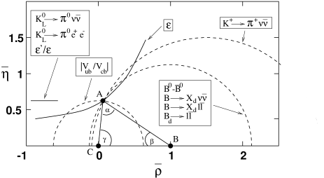
Figure 1: $K$ and $B$ physics constraints on the unitarity triangle in a world without errors (from [9]).

The need for a non-perturbative technique such as lattice QCD, to study the processes discussed above is clear: the simple free-quark picture of weak interactions is severely modified by the non-perturbative effects of the strong interaction. One of the most extreme examples of this is, of course, the $\Delta I=1/2$ rule in $K\to\pi\pi$ decays: decays in which isospin changes by $\Delta I=1/2$ are greatly enhanced over those in which the change is $\Delta I=3/2$. Using the operator product expansion (OPE) to separate short and long distance contributions, one finds that most of the enhancement, in a QCD based explanation, must come from non-perturbative QCD effects in the matrix elements, $\langle(\pi\pi)_{I=0,2}|\mathcal{H}_{\Delta S=1}|K^{0}\rangle$, of the effective, $\Delta S=1$ weak hamiltonian, $\mathcal{H}_{\Delta S=1}$ [10, 11].

The verification of this $\Delta I=1/2$ enhancement from first principles, as well as the calculation of $\epsilon^{\prime}/\epsilon$ and more generally the study of non-leptonic weak decays are some of the big challenges still facing lattice phenomenology. Though the problems these processes pose are many, much has been learned over the years:

1) The direct study of $K\to\pi\pi$ decays requires one to consider four-point functions. These correlation functions are statistically much more noisy than the two- and three-point functions encountered in most phenomenological studies undertaken on the lattice. To reduce the noise, one can consider transitions where all three particles are at rest or even study $K\to\pi$ (and $K\to 0$) transitions. In both cases, one uses chiral perturbation theory ($\chi$PT) to relate the quantities computed on the lattice to the physical matrix elements.

2) The renormalization of the dimension-six, four-quark operators which appear in the effective weak hamiltonian is difficult on the lattice:

$\bullet$ There is mixing with other dimension-six operators. Some of this mixing is the same as in the continuum. But with fermion formulations which break chiral symmetry explicitly, such as Wilson fermions, there is additional mixing with wrong chirality operators. This problem, however, is well understood and relatively well controlled.

$\bullet$ There is also mixing with lower-dimension operators. This gives rise to power divergences, proportional to inverse powers of $a$, where $a$ is the lattice spacing. The subtraction of these divergences is numerically very demanding. One must also be very careful. As pointed out some years ago by Martinelli, perturbation theory is likely to fail for such subtractions. Indeed, the coefficients of these divergences may have non-perturbative contributions of the form $e^{-\int^{g(a)}dg^{\prime}/\beta(g^{\prime})}=a\Lambda_{QCD}$, which are formally smaller than any term in a perturbative expansion. However, when enhanced by a power divergence, they can give a contribution which is of the same size as the physical quantity that is being calculated. A second concern is the definition of power subtracted operators in the presence of discretization errors. Again, a discretization error of, say, $\mathcal{O}\left(a\Lambda_{QCD}\right)$, on a linearly-divergent quantity with mass-dimension one may combine with this divergence and give a finite contribution of $\mathcal{O}\left(\Lambda_{QCD}\right)$.

Many tools have been developed over the years to address the problem of renormalization (for details, I refer you to Stefan Sint’s contribution):

$\bullet$ Lattice perturbation theory, performed in terms of a continuum-like, renormalized coupling constant can, in principle, be used to subtract mixings with same-dimension operators.

$\bullet$ CPS symmetry [12, 13], which is a discrete symmetry of many four-quark weak operators, is a powerful tool for classifying the mixings these operators may have. A CPS transformation is a CP transformation, followed by a switching transformation which changes $s$ into $d$ quarks and vice versa. This symmetry is of course broken, but only softly by terms proportional to powers of $(m_{s}-m_{d})$. There are also generalizations of CPS in which different pairs of quarks are swapped. I will generically refer to all of these transformations as CPS.

$\bullet$ Chiral symmetry, in the form of $\chi$PT or of the sytematic exploitation of chiral Ward identities can be used to guide, for instance, the subtraction of power divergences in $K\to\pi$ amplitudes for chirally symmetric lattice-fermion formulations [12] or the construction of effective weak hamiltonians in the case where the lattice fermions break chiral symmetry explicitly [14, 15].

$\bullet$ Chiral symmetry is not sufficient to determine the logarthmically divergent renormalizations required to make certain quark bilinears or quadrilinears finite. For these subtractions, a non-perturbative renormalization (NPR) technique was devised [16]. It is performed with quark states and makes use of a regularization-independent (RI) scheme. It requires gauge fixing and the existence of a window $\Lambda_{QCD}\ll\mu\ll\pi/a$, where $\mu$ is the renormalization scale. $\mu^{2}$ is usually taken to be the momentum squared of the quarks. $\Lambda_{QCD}\ll\mu$ is necessary to guarantee that the renormalization constants obtained are independent of the states used to calculate them. $\mu\ll\pi/a$ keeps discretization errors in check. This technique can also be used to compute the coefficient required to subtract the mixing of wrong-chirality operators in calculations involving four-quark operators.

$\bullet$ Another NPR technique has been developed, which makes use of a finite-volume, Schrödinger functional (SF) scheme [17]. It is associated with a non-perturbative renormalization group scaling and overcomes the problems encountered with the NPR techniques of [16]. It is gauge invariant, requires no window and is mass independent. It has not yet been applied to four-quark operators.

$\bullet$ Finally, to circumvent the mixing problem completely, the authors of [18] have suggested calculating the hadronic matrix element of the $T$-product of weak currents, $T\left\{J^{W}_{\mu}(x)J^{W\dagger}_{\mu}(0)\right\}$ for $a\ll|x|\ll 1/\Lambda_{QCD}$ on the lattice. The results would then be fitted to the continuum OPE, giving directly the matrix elements of the four-quark operators in the desired continuum scheme. Only the renormalization of bilinears would be necessary. The drawback is the need for very small lattice spacings which makes this approach costly numerically.

While much is already known, contributions are still being made to the problem of renormalization and mixing. Two new suggestions were proposed this year for obtaining $B_{K}$ with Wilson fermions but without the subtraction of wrong-chirality contributions usually required [19, 20]. The one-loop mixing of three- and four-quark operators with same-dimension operators has been analyzed in the domain-wall formalism [21, 22]. The renormalization of quark bilinears and four-quark operators, for domain-wall fermions, has been performed non-perturbatively in the RI scheme [23]. The same renormalization, for operators which have no power-divergences, has been performed at one loop for Neuberger fermions [24, 25].

3) A third problem is that present day lattices are only a few fermi long. On such lattices, it is not possible to separate the hadrons in a multiparticle state into asymptotic states.

4) A fourth problem is that the lattice method “only” provides approximate, euclidean correlation functions. This forces us to confront the “Maiani-Testa theorem” [26] which, in one of its guises, states that euclidean correlation functions which describe processes involving two or more final-state hadrons in the center of mass frame, yield amplitudes in which these particles are at rest. Thus, an euclidean correlation function chosen to describe $K\to\pi\pi$ decays will yield an amplitude for $K(\vec{0})\to\pi(\vec{0})\pi(\vec{0})$, which clearly has the wrong kinematics, unless $m_{K}=2m_{\pi}$. These statements will be made more precise below.

Both problems 3) and 4) can be addressed with $\chi$PT. For the first, $\chi$PT enables estimates of leading finite-volume corrections. It helps with the second problem in that it provides a means of extrapolating results to the correct physical point. In its quenched or partially quenched versions, it further gives a handle on quenching errors. There are new results in $\chi$PT this year which are directly relevant for lattice studies of weak decays of kaons and which I briefly review in Section 2.

While $\chi$PT seeks to correct finite-volume effects and problems resulting from the “Maiani-Testa theorem”, a new approach to non-leptonic weak decays was proposed this year. It uses the fact that lattice volumes are finite to circumvent the “Maiani-Testa theorem” and yield directly $K\to\pi\pi$ matrix elements from euclidean correlation functions [27]. Similar issues are currently being investigated by Lin et al. [28, 29].

Before closing this rather lenghty introduction, I would like to say a few words about domain-wall (and Neuberger) fermions, since they are beginning to play a prominent rôle in the study of light-hadron weak matrix elements. For details I refer you to Pavlos Vranas’ talk [30]. These two recent formulations of lattice fermions have a significant advantage over the more traditional Wilson and Kogut-Susskind formulations. They have a full chiral-flavor symmetry at finite lattice spacing. There is, of course, a price to pay. For domain-wall fermions it is a fifth dimension with $N_{5}\to\infty$ sites; for Neuberger fermions it is the inverse square root of a large matrix. The question then becomes: how small an $N_{5}$ or poor an approximation to the inverse square root can one take and still have sufficient chiral symmetry? Let me concentrate on domain-wall fermions, which are currently more commonly used for weak-interaction phenomenology. The assessment is somewhat mixed. The mathematical convergence in $N_{5}$, which is exponential asymptotically, can be rather slow for the couplings and volumes commonly used, though improvements can be made [31, 32]. However, it appears that in practice, for currently used simulation parameters, the chiral symmetry achieved may be sufficient for studying the physics of quarks whose masses are around that of the strange [33, 34, 35]. The criterion used in these studies is the residual mass, $m_{res}$, which essentially measures the amount the bare quark mass has to be shifted away from zero in order to have physically massless quarks. At $\beta=6.0$ with $N_{5}=16$ and on a $16^{3}\times 32$ lattice, the authors of [33] find that $m_{res}(\overline{\mbox{MS}},2\,\mbox{GeV})\simeq 4\mbox{MeV}$. Nevertheless, it should be kept in mind that the amount of chiral symmetry required will depend on the quantity studied. Indeed, the exponentially small chiral symmetry breaking can combine with power divergences induced by this breaking to give effects which may no longer be considered negligible. This problem is certainly relevant for matrix elements of four-quark operators whose mixings with lower-dimensional operators are often made significantly worse when chiral symmetry is broken explicitly. This issue is currently being addressed by the RBC collaboration [36].

Given the additional cost and potential difficulties of chirally-improved fermions, one is entitled to ask where, in weak matrix element calculations, is exact or nearly exact chiral symmetry absolutely necessary? This question is all the more justified that one appears to be able to access the desired physics with Wilson or Kogut-Susskind fermions in most cases. These calculations, however, are sufficiently complex and difficult that it is not clear, a priori, whether the overhead associated with chirally-improved fermions cannot be offset, at least partially, by their improved chiral behavior, by the fact that they are non-perturbatively $\mathcal{O}\left(a\right)$-improved, etc. It is thus important that all approaches be pursued.

The rest of this review is organized as follows. In Section 2, I review two new studies in $\chi$PT which are relevant for lattice calculations of weak decays of kaons. In Section 3, I discuss $K^{0}{-}\bar{K}^{0}$ mixing. A brief description of the $\Delta S=1$ effective hamiltonian is given in Section 4. Calculations of $K\to\pi\pi$ matrix elements from $K\to\pi$ and $K\to 0$ amplitudes are reviewed in Section 5, including two new ambitious studies using domain-wall fermions. In Section 6, I discuss some of the issues surrounding the calculation of physical $K\to\pi\pi$ matrix elements from lattice $K\to\pi\pi$ amplitudes. A new approach to the calculation of non-leptonic weak decays is presented in Section 7. Section 8 contains my conclusions.

The focus of this talk is on recent lattice developments. I will unfortunately not have the space to cover the results obtained by other methods. Please see [37] and references therein for descriptions of some of the other possible non-perturbative approaches.

2 Chiral perturbation theory results

There are at least two new studies in $\chi$PT this year which are directly relevant for lattice calculations of weak decays of kaons.

In the first, results for the one-loop, $\mathcal{O}\left(p^{2}\right)$ corrections to the $K\to\pi$ and $K\to\pi\pi$ matrix elements of the electroweak penguin operators $Q_{7}$ and $Q_{8}$ (see Eq. (17)), which belong to the $(8,8)$ representation of $SU(3)_{L}\times SU(3)_{R}$, were calculated [38]. The authors find that the $K\to\pi\pi$ amplitudes, including $\mathcal{O}\left(p^{2}\right)$ counterterms, can be obtained from a study of the $m_{K}^{2}$, $m_{\pi}^{2}$ and $p_{\pi}\cdot p_{K}$ dependence of $K\to\pi$ matrix elements. They further find that chiral loops can give rather significant ($+(27\pm 27)\%$) corrections to the $\mathcal{O}\left(p^{0}\right)$ results for $\langle(\pi\pi)_{I=2}|Q_{7,8}|K\rangle$. These results are obtained in regular $\chi$PT. It would be interesting to see how they are modified in quenched (q) or partially quenched (pq) $\chi$PT.

In the second study, it is one-loop corrections to the matrix elements of the $(8,1)$ and $(27,1)$ operators for $K\to\pi$ transitions at rest with degenerate $s$ and $d$ quarks and for $K\to 0$ with $m_{s}\neq m_{d}$, and the relation of these matrix elements to $K\to\pi\pi$ amplitudes, which are studied in pq$\chi$PT [39]. Not surprisingly, they find that $K\to\pi$ and $K\to 0$ amplitudes are not sufficient to determine all $\mathcal{O}\left(p^{4}\right)$ couplings required to obtain $K\to\pi\pi$ matrix elements at this order. Furthermore, they observe that the chiral logarithms are typically large and can depend strongly on $N_{sea}$. By using their results to guide extrapolations of lattice results for these amplitudes to the chiral limit, one can hope to obtain reliable results for the $\mathcal{O}\left(p^{2}\right)$ octet and twenty-seven-plet couplings, which are interesting quantities in their own right and for which a number of phenomenological estimates are available.

3 $K^{0}{-}\bar{K}^{0}$ mixing

The most general $\Delta S=2$ effective hamiltonian for $K^{0}{-}\bar{K}^{0}$ mixing can be written in terms of the following operators:

$$\mathcal{O}_{1} = [\bar{s}_{\alpha}d_{\alpha}]_{V-A}[\bar{s}_{\beta}d_{\beta}]_{V-A}$$

$$\mathcal{O}_{2} = [\bar{s}_{\alpha}d_{\alpha}]_{S-P}[\bar{s}_{\beta}d_{\beta}]_{S-P}$$

$$\mathcal{O}_{3} = [\bar{s}_{\alpha}d_{\beta}]_{S-P}[\bar{s}_{\beta}d_{\alpha}]_{S-P}$$ (1)

$$\mathcal{O}_{4} = [\bar{s}_{\alpha}d_{\alpha}]_{S-P}[\bar{s}_{\beta}d_{\beta}]_{S+P}$$

$$\mathcal{O}_{5} = [\bar{s}_{\alpha}d_{\beta}]_{S-P}[\bar{s}_{\beta}d_{\alpha}]_{S+P}\ ,$$

where $\alpha$ and $\beta$ are color indices. In the SM, only $\mathcal{O}_{1}$ contributes; in extensions, such as the MSSM, the other operators may also be required.

These operators have positive and negative parity components, and only the former contribute to $K^{0}{-}\bar{K}^{0}$ mixing. For instance,

$$\mathcal{O}_{1}=\mathcal{O}_{VV+AA}-2\mathcal{O}_{VA}\ ,$$ (2)

and $\mathcal{O}_{VV+AA}$ determines the SM contributions to this mixing. As is well known, the explicit chiral symmetry breaking present in the Wilson formulation of fermions implies that $\mathcal{O}_{VV+AA}$ will have finite mixings with wrong chirality operators:

$$\mathcal{O}_{VV+AA}(\mu)=Z_{VV+AA}(a\mu,g^{2})$$ (3)

$$\times\left\{\mathcal{O}_{VV+AA}(a)+\sum_{i}\Delta_{i}(g^{2})\mathcal{O}_{i}\right\}\ ,$$

with $i=VV-AA,\,SS+PP,\,SS-PP,\,TT$. This mixing is particularly bad here because $\mathcal{O}_{VV+AA}$ is subdominant in the chiral expansion.

3.1 Two proposals for getting around mixing with wrong chirality operators

As shown by Bernard and collaborators many years ago, CPS symmetry protects the parity odd components of the operators in Eq. (1) from mixing with operators of wrong chirality [13]. Thus,

$$\mathcal{O}_{VA}(\mu)=Z_{VA}(a\mu,g^{2})\mathcal{O}_{VA}(a)\ .$$ (4)

So the basic idea behind these proposals is to relate the matrix element of interest, $\langle\bar{K}^{0}|\mathcal{O}_{VV+AA}|K^{0}\rangle$, to a correlation function where the only four-quark operator is $\mathcal{O}_{VA}$.

The basic ingredient is the chiral rotation [19]

$$\left(\begin{array}[]{c}u\\ d\end{array}\right)\to\mathrm{exp}\left[i\alpha\gamma_{5}\tau^{3}/2\right]\left(\begin{array}[]{c}u\\ d\end{array}\right)\ .$$ (5)

It is implemented in two different ways.

In the first, one considers twisted-mass QCD [40]:

$$\mathcal{L}=\bar{\psi}\left(D_{W}+m_{0}+i\mu_{0}\gamma_{5}\tau^{3}\right)\psi$$ (6)

$$+\bar{s}\left(D_{W}+m_{0}^{s}\right)s\ ,$$

where $D_{W}$ is the usual Wilson Dirac operator, $\psi$ is the $(u,d)$ doublet and $m_{0}$, $\mu_{0}$ and $m_{0}^{s}$ are bare mass parameters. In the continuum, this lagrangian would be equivalent to the usual, three-flavor QCD lagrangian. On the lattice, however, because of the Wilson term, it is not. The authors then suggest adjusting the renormalized mass $m$ and twisted mass $\mu$ in such a way that the angle of the rotation, $\alpha$, in Eq. (5) is $\pi/2$. Then, the physical $\mathcal{O}_{VV+AA}$ is $-2\mathcal{O}_{VA}$ in the twisted theory, which means that only a multiplicative renormalization is required.

The authors of [20] consider a Ward identity associated with an infinitesimal version of the rotation of Eq. (5):

$$Z_{P}\,\langle P(t_{1})\mathcal{O}_{VV+AA}(\mu;0)P(t_{2})\rangle=Z_{VA}(a\mu)$$

$$\times\bigl{[}2m\,Z_{P}\sum_{x}\langle\Pi(x)P(t_{1})\mathcal{O}_{VA}(a;0)P(t_{2})\rangle$$

$$-Z_{S}\langle S(t_{1})\mathcal{O}_{VA}(a;0)P(t_{2})\rangle$$ (7)

$$-Z_{S}\langle P(t_{1})\mathcal{O}_{VA}(a;0)S(t_{2})\rangle\bigr{]}+\mathcal{O}\left(a\right)\ ,$$

with $P=\sum_{\vec{x}}\bar{d}\gamma_{5}s$, $S=\sum_{\vec{x}}\bar{d}s$, $\Pi=\bar{d}\gamma_{5}d-\bar{u}\gamma_{5}u$ and $m=Z_{A}\langle 0|\partial_{\mu}A_{\mu}^{\pi}|\pi^{0}\rangle/2\langle 0|P^{\pi}|\pi^{0}\rangle$.

Correlators containing the operator $S$ are exponentially suppressed for $t_{1},\,-t_{2}\to\infty$, since they are dominated by scalar instead of pseudoscalar contributions. Thus, the correlator $\sum_{x}\langle\Pi(x)P(t_{1})\mathcal{O}_{VA}(0)P(t_{2})\rangle$ yields $\langle\bar{K}^{0}|\mathcal{O}_{VV+AA}(\mu)|K^{0}\rangle$ without mixing. Exploratory results for $B_{K}$ using this method were presented at this conference [8].

Both methods are generalizable to other matrix elements. Of course, none of this is necessary with fermion formulations which have a chiral symmetry, such as domain-wall, Neuberger or Kogut-Susskind fermions.

3.2 Matrix elements for $K^{0}{-}\bar{K}^{0}$ mixing beyond the Standard Model

Donini et al. have computed the matrix elements of all operators of Eq. (1) between $K^{0}$ and $\bar{K}^{0}$ states [6]. They work with a tree-level, $\mathcal{O}\left(a\right)$-improved Sheikholeslami-Wohlert (SW) action at $\beta=6.0$ and 6.2, in the quenched approximation. Their strange and down quarks are degenerate. They renormalize the matrix elements non-perturbatively in the RI scheme, match them onto other schemes at one loop and run them at two loops.

To quantify and subtract residual artifacts that might remain in chiral behavior of the matrix element of $\mathcal{O}_{1}$, they fit its dependence on mass and momenta to the form:

$$\frac{\langle\bar{K}^{0}|\mathcal{O}_{1}(\mu)|K^{0}\rangle}{\frac{8}{3}f_{K}^{2}}=\alpha+\beta m_{K}^{2}+\gamma p_{K}\cdot p_{\bar{K}}+\cdots\ ,$$ (8)

where the parameters $\alpha$ and $\beta$ are pure artifacts and the dots include higher-order terms in the chiral expansion to which they are not sensitive numerically.  $B_{K}$ is then simply $\gamma$.

In analogy with the definition of $B_{K}=\langle\bar{K}^{0}|\mathcal{O}_{1}|K^{0}\rangle/\frac{8}{3}f_{K}^{2}m_{K}^{2}$, they suggest the following normalization for the matrix elements of the other operators ($i=2,\cdots,5$):

$$\tilde{B}_{i}(\mu)=\frac{\langle\bar{K}^{0}|\mathcal{O}_{i}(\mu)|K^{0}\rangle}{f_{K}^{2}m_{K^{*}}^{2}}\ ,$$ (9)

instead of the usual, vacuum saturation approximation (VSA) normalization, which is traditionally expressed in terms of the quark-mass combination $[m_{s}(\mu)+m_{d}(\mu)]^{2}$. The problem with giving the matrix elements in units of their VSA values is that they are then used, in phenomenological applications, with uncorrelated values of the quark masses, thus compounding the uncertainty on the matrix elements with those on the poorly measured quark masses. This problem obviously disappears with the normalization of Eq. (9).

The authors do observe some lattice spacing dependence in their results, which never exceeds two statistical standard deviations. They choose to average their $\beta=6.0$ and 6.2 results and keep the largest statistical error. Their final results are summarized in Table 1. It is worth noting that at $2\,\mbox{GeV}$ in the $\overline{\mbox{MS}}$-NDR scheme, the non-SM matrix elements are typically 2 to 12 times larger than the matrix element of $\mathcal{O}_{1}$.

Table 1: Matrix elements of the $\Delta S=2$ operators of Eq. (1) between $K^{0}$ and $\bar{K}^{0}$ states as obtained in [6] in the RI scheme. Also given are the corresponding renormalization group invariant (RGI) matrix elements, as defined in [6].

$\langle\mathcal{O}_{i}\rangle$	RI ($\mu=2\,\mbox{GeV}$)	RGI
$\langle\mathcal{O}_{1}\rangle$	$0.012(3)\,\mbox{GeV}^{4}$	$0.017(4)\,\mbox{GeV}^{4}$
$\langle\mathcal{O}_{2}\rangle$	$-0.077(10)\,\mbox{GeV}^{4}$	$-0.050(7)\,\mbox{GeV}^{4}$
$\langle\mathcal{O}_{3}\rangle$	$0.024(3)\,\mbox{GeV}^{4}$	$0.001(7)\,\mbox{GeV}^{4}$
$\langle\mathcal{O}_{4}\rangle$	$0.142(12)\,\mbox{GeV}^{4}$	$0.068(6)\,\mbox{GeV}^{4}$
$\langle\mathcal{O}_{5}\rangle$	$0.034(5)\,\mbox{GeV}^{4}$	$0.038(5)\,\mbox{GeV}^{4}$

The result $\langle\mathcal{O}_{1}\rangle$ in Table 1 corresponds to the following value for $B_{K}$:

$$B_{K}^{NDR}(2\,\mbox{GeV})=0.68(21)\ .$$ (10)

3.3 $B_{K}$ with domain-wall fermions

As already pointed out above, chiral symmetry facilitates the calculation of $B_{K}$. Domain-wall fermions are thus a good candidate for such a calculation. The first study of $B_{K}$ with domain-wall fermions was actually performed some years ago [41]. Two new quenched results were presented at this conference, by the CP-PACS [4] and the RBC [5] collaborations. Both calculations are performed with Shamir’s variant of domain-wall fermions and degenerate $s$ and $d$ quarks with masses approximatively ranging from $m_{s}/4$ to $m_{s}$. They differ, however, in the gauge action employed. CP-PACS use an RG-improved action at two values of $\beta=2.6$ and 2.9, corresponding to an inverse lattice spacing of $1.81(4)\,\mbox{GeV}$ and $2.87(7)\,\mbox{GeV}$, respectively, as determined from the $\rho$-meson mass. RBC used a standard Wilson plaquette action, with $\beta=6.0$, corresponding to an inverse lattice spacing of roughly $2\,\mbox{GeV}$. Another important difference in the calculations is that RBC renormalize the matrix element non-perturbatively [23], using the techniques of [16], while CP-PACS match their results onto the continuum perturbatively, at one loop [21].

CP-PACS perform a rather extensive study of the dependence of their results on fifth-dimensional and spatial sizes and on cutoff. At $\beta=2.6$, they work with the following four lattices: $(16{-}24{-}32)^{3}\times 40\times 16$ and $24^{3}\times 40\times 32$. At $\beta=2.9$, they have the two lattices $(24{-}32)^{3}\times 60\times 16$. To investigate the chiral properties of their $\Delta S=2$ matrix element, they consider the ratio

$$B_{P}=\frac{\langle\bar{K}^{0}|\mathcal{O}_{1}|K^{0}\rangle}{\langle\bar{K}^{0}|\bar{s}\gamma_{5}d|0\rangle\langle 0|\bar{d}\gamma_{5}s|K^{0}\rangle}\ ,$$ (11)

which should vanish, by chiral symmetry, in the limit $m_{K}\to 0$. They study $B_{P}$ in the limit of vanishing quark mass, obtained by linear extrapolation from finite quark mass. They find that extending the fifth dimension by a factor of two, from 16 to 32 points, does not reduce the deviation of $B_{P}$ from zero which they observe. Going to smaller lattice spacing does not reduce the effect either whereas increasing the volume does. The effect is of order -10 to -20% in units of $B_{P}$ at $m_{K}$ on their $(32{-}24{-}16)^{3}\times 40\times 16$ lattices.  They conclude that the deviation of $\langle\bar{K}^{0}|\mathcal{O}_{1}|K^{0}\rangle$ from zero at vanishing quark mass must be a finite-volume effect. This is supported by the fact that the volume dependence of $B_{P}$ at finite mass increases rapidly as this mass is reduced. At $m_{K}$, the reduction in $B_{P}$ in going from the largest to the smallest volume is small, less than 2%. At $am_{q}=0.01$, it is approximatively 15%.

They then study the mass-dependence of $B_{K}$, and interpolate to the kaon mass using the following $\chi$PT-inspired functional form

$$B_{K}=B(1-3c\times am_{q}\,\mathrm{ln}(am_{q})+b\times am_{q})\ ,$$ (12)

as shown in Figure 2 for their $24^{3}\times 40\times 16$ lattice. The physical point is obtained at half the strange quark mass, as estimated from the experimental value of $m_{K}/m_{\rho}$. The value of $B_{K}$ extrapolated to the chiral limit appears to be approximatively 30% smaller than the value at $m_{K}$, which would help reconcile lattice results with the chiral-limit result for $B_{K}$ obtained recently in a large-$N_{c}$ approximation to QCD [42]. However, it is important to note that finite-volume effects of the kind described above could significantly distort the chiral extrapolation of $B_{K}$. If so, an extrapolation to infinite volume would be necessary to determine $B_{K}$ reliably in the chiral limit.

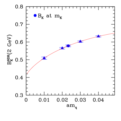
Figure 2: Dependence of $B_{K}^{NDR}(2\,\mbox{GeV})$ on bare quark mass, from CP-PACS [4].

Finally, they study the dependence of $B_{K}$ at $m_{K}$ on lattice-spacing, spatial volume and fifth dimensional size. They find that these dependences are small. They obtain the following result for $B_{K}$

$$B_{K}^{NDR}(2\,\mbox{GeV})=0.575(6)\ ,$$ (13)

by fitting, to a constant in lattice spacing, the results that they obtain from their runs on a $24^{3}\times 40\times 16$ lattice at $\beta=2.6$ and on a $32^{3}\times 60\times 16$ lattice at $\beta=2.9$. Errors in Eq. (13) are statistical only.

From their fixed lattice spacing calculation on a $16^{3}\times 32\times 16$ lattice, the RBC collaboration obtain the following result for $B_{K}$:

$$B_{K}^{NDR}(2\,\mbox{GeV})=0.538(8)\ .$$ (14)

This result is lower than the CP-PACS result. This difference may be due to the fact that RBC renormalize their results perturbatively whereas CP-PACS do so perturbatively. The non-perturbative matching coefficient used by RBC is 7% smaller than the corresponding mean-field improved, one-loop coefficient computed in [21].

3.4 $B_{K}$ summary

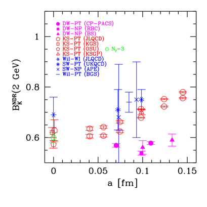
Figure 3: $B_{K}^{NDR}(2\,\mbox{GeV})$ with domain-wall (filled symbols), Kogut-Susskind (open symbols) and Wilson/Sheikholeslami-Wohlert (stick symbols) fermions. All results are quenched except for the $N_{f}=3$ result of OSU and all errors are statistical. PT stands for perturbative matching, NP for non-perturbative matching à la [16] and WI, for matching using Ward identities. The references for the different results are: CP-PACS [4], RBC [5], BS [41] (with NPR, hep-lat/9909108), JLQCD (KS) [43], KGS [44], OSU and $N_{f}=3$ [45], KSGP [46], JLQCD (Wil) [47], UKQCD [48], APE [6], BGS [49].

I summarize, in Figure 3, the results for $B_{K}^{NDR}(2\,\mbox{GeV})$ obtained by different collaborations with different fermion formulations. The size of the error bars on the Wilson results is mostly a reflection of the subtractions which are necessary to restore correct chiral behavior. The fact that different actions give different results at fixed lattice spacing is a sign that for some of the formulations at least, there is still some way to the continuum limit. In this limit, however, all formulations agree within one and some standard deviations. The domain-wall results exhibit rather good scaling. They are also systematically lower at fixed lattice spacing. If this trend survives further scrutiny of the continuum extrapolation and of systematic effects, we may have to slightly revise our canonical estimate of $B_{K}$. However, for the moment, because it involves the most extensive study of systematic errors, the KS result of the JLQCD collaboration [43] should still be taken as the reference result. To this one must add uncertainties due to quenching and the fact that the down and strange quarks are degenerate in the calculation. Sharpe [50], on the basis of q$\chi$PT and the preliminary “$N_{f}=3$” OSU results [45], suggests an enhancement factor of $1.05\pm 0.15$ to “unquench” quenched results for $B_{K}$. He advocates an additional factor $1.05\pm 0.05$ to compensate for the effect of working with degenerate quark masses. Here, we choose to keep his estimate of errors, but not use his enhancement factors so as not to modify the central value on the basis of information which is, for the most part, not provided by lattice calculations. Thus, we quote

$$B_{K}^{NDR}(2\,\mbox{GeV})=0.628(42)(99)$$ (15)

$$\to\hat{B}_{K}^{NLO}=0.86(6)(14)\ ,$$

where $\hat{B}_{K}^{NLO}$ is the two-loop RGI $B$-parameter obtained from $B_{K}^{NDR}(2\,\mbox{GeV})$ with $N_{f}=3$ and $\alpha_{s}(2\,\mbox{GeV})=0.3$. Of course, future studies should investigate systematically the effect of including light flavors of dynamical quarks.

4 $K\to\pi\pi$ decays: general considerations

With all massive modes, including charm, integrated out, the $\Delta S=1$ effective hamiltonian is given by 

$$\mathcal{H}_{\Delta S=1}=\frac{G_{F}}{\sqrt{2}}V_{ud}V_{us}^{*}\sum_{i=1}^{10}(z_{i}+\tau y_{i})Q_{i}\ ,$$ (16)

where $z_{i}$ and $y_{i}$ are short-distance coefficients, $\tau=-V_{ts}^{*}V_{td}/V_{us}^{*}V_{ud}$ and

$$Q_{1} = (\bar{s}_{\alpha}u_{\beta})_{V-A}\;(\bar{u}_{\beta}d_{\alpha})_{V-A}$$

$$Q_{2} = (\bar{s}u)_{V-A}\;(\bar{u}d)_{V-A}$$

$$Q_{3,5} = (\bar{s}d)_{V-A}\sum_{q}(\bar{q}q)_{V\mp A}$$

$$Q_{4,6} = (\bar{s}_{\alpha}d_{\beta})_{V-A}\sum_{q}(\bar{q}_{\beta}q_{\alpha})_{V\mp A}$$ (17)

$$Q_{7,9} = {3\over 2}\;(\bar{s}d)_{V-A}\sum_{q}e_{q}\;(\bar{q}q)_{V\pm A}$$

$$Q_{8,10} = {3\over 2}\;(\bar{s}_{\alpha}d_{\beta})_{V-A}\sum_{q}e_{q}(\bar{q}_{\beta}q_{\alpha})_{V\pm A}\ ,$$

with $q=u,d,s$. It proves useful to split the $\Delta S=1$ operators into a sum of operators which transform under irreducible representations of the isospin group: $Q_{i}=Q_{i}^{1/2}+Q_{i}^{3/2}$.

Integrating out charm is questionable since $m_{c}\sim 1.3\,\mbox{GeV}$. Above the charm threshold, one has the following effective hamiltonian:

$$\mathcal{H}^{c}_{\Delta S=1} = \frac{G_{F}}{\sqrt{2}}V_{ud}V_{us}^{*}\left[(1-\tau)\sum_{i=1}^{2}z_{i}(Q_{i}-Q_{i}^{c})\right.$$ (18)

$$\left.+\tau\sum_{i=1}^{10}(z_{i}+y_{i})Q_{i}\right]\ ,$$

where $Q_{1,2}^{c}=Q_{1,2}[u\to c]$, the sum over $q$ now runs over $u,d,s,c$ and $y_{i}$ and $z_{i}$ are given $N_{f}=4$ values.

The rôle of the lattice is to compute:

$$\langle Q_{i}\rangle_{I}\equiv\langle(\pi\pi)_{I}|Q_{i}|K\rangle$$ (19)

for the two isospin channels $I=0,2$ and $i=1,\cdots,10$, where $Q_{1,2}$ in Eq. (19) are to be understood as $Q_{1,2}-Q_{1,2}^{c}$ in the case of an active charm. 

5 $K\to\pi\pi$ from $K\to\pi$ and $K\to 0$

The idea here is to compute three-point functions to obtain matrix elements of $\Delta S=1$ operators between $K$ and $\pi$ states, where the light quarks typically have masses around $m_{s}/2$, and then use $\chi$PT to relate them to the corresponding, physical $K\to\pi\pi$ matrix elements. This last step is usually performed at lowest non-trivial order. In the case of $\Delta I=1/2$ transitions, there is an unphysical contribution to $K\to\pi$ matrix elements of $(8,1)$ operators which does not appear in its physical $K\to\pi\pi$ counterpart. This contribution can be subtracted by considering $K\to 0$ transitions [12].

5.1 Electroweak penguins with quenched Wilson fermions

As part of their study of $\Delta S=2$ matrix elements, Donini et al. [6] have computed the $\Delta I=3/2$, electroweak-penguin matrix elements, $\langle Q_{7,8}\rangle_{2}$, which give important contributions to $\mathrm{Re}\;\epsilon^{\prime}/\epsilon$. The parameters of the calculation are the same as those presented in Section 3.2.

They use leading order $\chi$PT to get the $K\to\pi\pi$ matrix elements in the chiral limit through

$$\langle Q_{7,8}\rangle_{2}=\frac{\sqrt{3}m_{\rho}^{2}f_{\pi}}{2}\lim_{m_{q}\to 0}\tilde{B}_{5,4}\ ,$$ (20)

which they obtain by linear extrapolation of their $K^{0}-\bar{K}^{0}$ results calculated for degenerate quark masses, $m_{s}=m_{d}=m_{q}$. Here, $f_{\pi}=131\,\mbox{MeV}$. They find, in the chiral limit and at $2\,\mbox{GeV}$ in the NDR-$\overline{\mbox{MS}}$ scheme: 

$$\begin{array}[]{l}\langle Q_{7}(2\,\mbox{GeV})\rangle_{2}^{NDR}/(m_{\rho}^{2}f_{\pi})=1.7(3)\ ,\\ \langle Q_{8}(2\,\mbox{GeV})\rangle_{2}^{NDR}/(m_{\rho}^{2}f_{\pi})=8.1(8)\ .\end{array}$$ (21)

These values are obtained by one-loop matching from their non-perturbatively renormalized results in the RI scheme. This matching is rather poorly behaved as it induces a 40% change in $\langle Q_{7}\rangle_{2}$ and a 27% change in $\langle Q_{8}\rangle_{2}$. Since all other results for these matrix elements are, to date, normalized by their vacuum saturation value and this value is not provided, I will not attempt a comparison with Eq. (21).

5.2 Matrix elements of the $\Delta S=1$ operators from quenched domain-wall QCD

At this conference, the CP-PACS [51] and RBC [5, 36] collaborations presented preliminary results from calculations of the matrix elements of all 10, $\Delta S=1$ operators. They use domain-wall fermions and work in the quenched approximation. They are also considering the case of active charm. Both collaborations work on lattices of size $16^{3}\times 32\times 16$, with a domain-wall height $M=1.8$ and cutoffs $a^{-1}\simeq 2\,\mbox{GeV}$. In addition to a Wilson plaquette action at $\beta=6.0$ used by the two teams, CP-PACS also perform the calculation with a RG-improved action at $\beta=2.6$.  In these calculations, a pseudoscalar meson composed of degenerate quarks of bare mass $am_{q}\sim 0.02$ would have a mass close to that of the physical kaon. While CP-PACS renormalize their matrix elements at one loop [22], RBC perform this renormalization non-perturbatively [23].

$\Delta I=3/2$ transitions involve no “penguin” contractions and therefore no mixing with lower dimensional operators. And because of the approximate chiral symmetry of domain-wall fermions, the structure of the renormalization is the same as in the continuum, up to corrections which are exponentially small in $N_{5}$.

$\Delta I=1/2$ transitions can receive contributions from lower dimensional operators. To leading order in the chiral expansion, the matrix elements $\langle\pi^{+}|Q_{i}^{1/2}(a)|K^{+}\rangle$, $i\neq 7,8$, are quadratically divergent due to mixing with the operator

$$\mathcal{O}_{sub}=(m_{s}+m_{d})\bar{s}d-(m_{s}-m_{d})\bar{s}\gamma_{5}d\ .$$ (22)

To subtract this divergence, one uses the fact that the coefficients of the parity even and odd components of $\mathcal{O}_{sub}$ are fixed by chiral and CPS symmetry [12]. Then one constructs a subtracted operator $Q_{i}-\alpha_{i}\mathcal{O}_{sub}$ by imposing the constraint

$$\langle 0|Q_{i}-\alpha_{i}\mathcal{O}_{sub}|K^{0}\rangle=0\ ,$$ (23)

to determine $\alpha_{i}$. Because CP-PACS works with degenerate quarks, they obtain $\alpha_{i}$ from a derivative of Eq. (23) with respect to $m_{s}$ at the point $m_{s}=m_{d}$. RBC work with $m_{s}\neq m_{d}$ and obtain $\alpha_{i}$ from the slope in $m_{s}-m_{d}$.

Note that this construction relies heavily on the fact that the coefficients of $\bar{s}d$ and $\bar{s}\gamma_{5}d$ in $\mathcal{O}_{sub}$ are fixed. In the absence of chiral symmetry, as when using Wilson fermions, this is no longer the case and one finds that the matrix elements discussed above are cubically divergent due to mixing with $\bar{s}d$ and that the coefficient of this divergence cannot be obtained by studying $K\to 0$ matrix elements.

Using leading order $\chi$PT, CP-PACS relate the $K\to\pi$ matrix elements that they calculate to the desired $K\to\pi\pi$ matrix elements, through:

$$\langle Q_{i}\rangle_{I}=C_{I}f_{\pi}(m_{K}^{2}-m_{\pi}^{2})\sum_{k}\frac{Z_{ik}}{Z_{A}^{2}}$$ (24)

$$\times\left[\frac{\langle\pi^{+}|Q_{k}^{\Delta I}-\alpha_{k}^{\Delta I}\mathcal{O}_{sub}|K^{+}\rangle}{\langle\pi^{+}|\bar{u}\gamma_{0}\gamma_{5}d|0\rangle\langle 0|\bar{s}\gamma_{0}\gamma_{5}u|K^{+}\rangle}\right]_{\chi}{\rm[GeV^{3}]}$$

$$\langle Q_{j}\rangle_{I}=-C_{I}f_{\pi}\sum_{k}\frac{Z_{jk}}{Z_{A}^{2}}$$ (25)

$$\times\left[m_{P}^{2}\,\frac{\langle\pi^{+}|Q_{k}^{\Delta I}|K^{+}\rangle}{\langle\pi^{+}|\bar{u}\gamma_{0}\gamma_{5}d|0\rangle\langle 0|\bar{s}\gamma_{0}\gamma_{5}u|K^{+}\rangle}\right]_{\chi}{\rm[GeV^{3}]}\ ,$$

with $i=1,2,\cdots,6,9,10$, $j=7,8$ and where $\Delta I=1/2(3/2)$ and $C_{I}=\sqrt{3/2}(\sqrt{3})$ for $I=0(2)$. The $Z_{ij}/Z_{A}^{2}$ are the constants required to match the lattice results onto the NDR-$\overline{\mbox{MS}}$ scheme. $\alpha_{i}^{3/2}=0$ and $\alpha_{i}^{1/2}$ is obtained as described around Eq. (23). $m_{P}$ is the mass of the pseudoscalar meson in the simulation. $[\ldots]_{\chi}$ indicates that the term in brackets is linearly extrapolated to the chiral limit.

Their results for the plaquette and RG-improved actions are very similar. We will therefore concentrate on the former, because they can be compared directly to RBC’s results, obtained with the same parameters.

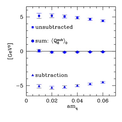
Figure 4: Subtraction of the quadratic divergence which appears in the construction of $\langle Q_{6}\rangle_{0}$ given in Eq. (24), for different values of the degenerate quark mass, $m_{q}$.

Figure 4 shows the subtraction of the power divergence in the calculation of $\langle Q_{6}\rangle_{0}$ performed by CP-PACS, as a function of their degenerate quark mass. The cancellation is severe and leads to a value for $\langle Q_{6}^{sub}\rangle_{0}$  which is very roughly 40 times smaller than the individual contributions. That a signal remains at all must be due to the strong statistical correlation between the two terms.

While CP-PACS presented preliminary results for the matrix elements, $\langle Q_{i}(2\,\mbox{GeV})\rangle_{I}^{NDR}$, with $i=1,\cdots 10$, and $I=0,2$, it is important to remember that this is a very difficult calculation and that premature phenomenological consequences should not be drawn. I have therefore chosen not to quote these results here. Let me instead comment on the problems they may be confronted with.

One of the features of their results is that some of the $\alpha_{s}$ corrections in the matching of $\langle Q_{i}^{sub}\rangle_{0}$ onto the NDR-$\overline{\mbox{MS}}$ scheme are large, as large as 50% in some instance. It will be interesting to see what RBC finds with its non-perturbative matching.

Also, as mentioned above, the fact that the divergence is quadratic in the $\Delta I=1/2$ channel is a consequence of chiral symmetry. Because chiral symmetry is only approximate with domain-wall fermions, we actually expect there to be a cubic divergence due to mixing with $\bar{s}d$, as in the Wilson fermion case. However, instead of being of order 1, the coefficient of this divergence will be exponentially small, leading to a term of the form $e^{-cN_{5}}\bar{s}d/a^{3}$, which is formally of order $m_{res}\bar{s}d/a^{2}$. Such a term will not be subtracted by the condition of Eq. (23). It will appear as a non-vanishing intercept at $m_{q}=-m_{res}$ in a plot of the matrix element versus quark mass of an operator such as $Q_{6}$, which should vanish in the chiral limit. Such an intercept is seen by RBC, as shown in Figure 5.

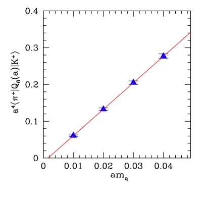
Figure 5: $K^{+}\to\pi^{+}$ matrix element of the bare operator $Q_{6}$. The line corresponds to an uncorrelated linear fit to the data.

This intercept is still reasonably small on the scale of the unsubtracted $\langle\pi^{+}|Q_{6}(a)|K^{+}\rangle$ matrix element of Figure 5, at the values of $am_{q}$ at which the calculation is performed. However, it is large when converted to the scale of $\langle Q_{6}^{sub}\rangle_{0}$ in Figure 4 and increases like $1/m_{P}^{2}$ when $m_{P}$ is decreased, as the definition of Eq. (24) implies.  Of course, the estimate of the size of this unphysical contribution will depend sensitively on how the chiral extrapolation of $\langle\pi^{+}|Q_{6}(a)|K^{+}\rangle$ is performed, a delicate question in quenched QCD and in a finite volume.  But this should be taken as a warning that such effects may be important and should not be ignored. One way to subtract such an unphysical intercept is to obtain the chiral-limit matrix element from the slope in the dependence of $\langle\pi^{+}|Q_{6}^{sub}|K^{+}\rangle$ on $m_{q}$. This is the procedure advocated by RBC [36] and I would favor it over the use of Eq. (24).

It should also be remembered that what is calculated are $K\to\pi$ matrix elements where the $K$ and the $\pi$ are degenerate and at rest. These matrix elements, suitably normalized, are then extrapolated to the chiral limit and translated into $K\to\pi\pi$ matrix elements using leading order $\chi$PT. This procedure thus requires a good control over chiral extrapolations, which is not trivial in the quenched approximation and in a finite volume.  Furthermore, the leading order $\chi$PT relations between $K\to\pi$ and $K\to\pi\pi$ neglect effects which may be important, such as final-state interactions.

Finally, results involving an active charm quark have not yet been presented. Given the fact that the charm is not that heavy, its contribution as an active quark may be important.

6 $K\to\pi\pi$ from unphysical $K\to\pi\pi$

This approach is complementary to the $K\to\pi$ and $K\to 0$ method discussed above. Here, four-point functions are used to compute the matrix elements for $K\to\pi\pi$ transitions at unphysical values of the mesons’ masses and momenta, imposed by computational and theoretical limitations. Then, low order $\chi$PT is used to extrapolate the result to the physical point. While this method is numerically more demanding because of the four-point functions required, renormalization is simplified. In fact, this approach appears to be the only one possible when considering $\Delta I=1/2$ transitions in the absence of the GIM mechanism (as is the case when studying $\epsilon^{\prime}$) with fermions which explicitly break chiral symmetry, such as Wilson fermions.

The SPQcdR collaboration are undertaking a quenched study of the $\Delta I=1/2$ rule and of $\epsilon^{\prime}$ using non-perturbatively $\mathcal{O}\left(a\right)$-improved Wilson fermions [8] and NPR matching à la [16]. All mesons are taken at rest. They work with degenerate quarks, i.e. $m_{u}=m_{d}=m_{s}$, but consider also the situation where the quarks in the kaon and in the pions have masses tuned so that $m_{K}=2m_{\pi}$. With pions at rest, this latter situation yields $K\to\pi\pi$ at threshold.

In the $\Delta I=3/2$ channel, renormalization is particularly simple as there is no mixing with lower-dimension operators and CPS symmetry guarantees that there is no mixing with wrong-chirality operators of dimension six [13]. They presented an exploratory study of the matrix element $\langle Q_{2}+Q_{1}\rangle_{2}$, which constitutes the denominator of the $\Delta I=1/2$ rule. This amplitude has already been studied in the quenched approximation with unimproved Wilson fermion, perturbative matching and degenerate quarks [52, 53, 54], as reviewed last year [55]. By accounting for finite-volume effects and chiral logarithms [66], and using modern techniques in perturbative renormalization, the authors of the most recent study [54] were able to reconcile, with experiment, the physical amplitude obtained from the chiral-limit lattice results. The pioneering studies of [52, 53] had found a discrepancy by a factor of roughly two. Non-perturbative matching and $\mathcal{O}\left(a\right)$-improvement, as well as the situation where $m_{K}=2m_{\pi}$, as considered by SPQcdR, should help further clarify the situation for these decays.

SPQcdR also presented exploratory results from the first $K\to\pi\pi$ calculation of the amplitudes $\langle Q_{7,8}\rangle_{2}$ [8]. Combining their results with those obtained from $K\to\pi$ amplitudes should help obtain more reliable predictions for these matrix elements.

In the $\Delta I=1/2$ channel, SPQcdR are considering mixing with the lower dimension operators 

$$\mathcal{O}_{P} = (m_{s}-m_{d})\bar{s}\gamma_{5}d$$ (26)

$$\tilde{\mathcal{O}}_{G} = (m_{s}-m_{d})\bar{s}\sigma_{\mu\nu}\tilde{G}_{\mu\nu}d\ ,$$

where the factor of $(m_{s}-m_{d})$ is required by CPS symmetry. (The $\Delta S=1$ operators of Eq. (17) are all even under CPS.) Clearly, working with $m_{u}=m_{d}=m_{s}$ eliminates this mixing completely [13]. It is shown in [18] that the choice $m_{K}=2m_{\pi}$ with all mesons at rest also simplifies the renormalization because no momentum is transfered by the $\Delta S=1$ operator. SPQcdR is pursuing both these avenues [8].

7 Non-leptonic weak decays from finite-volume correlation functions

Determinations of $K\to\pi\pi$ amplitudes, both from $K\to\pi$ (and $K\to 0$) matrix elements and from unphysical $K\to\pi\pi$ amplitudes, rely on low order $\chi$PT. They therefore neglect chiral corrections which may be important. Aside from this limitation, it would be satisfying to be able to calculate $K\to\pi\pi$ amplitudes in full, directly on the lattice. Can this be done?

7.1 Euclidean correlation functions and the “Maiani-Testa no-go theorem”

The lattice method provides approximate estimates of euclidean correlation functions. While the Osterwalder-Schrader theorem guarantees that these correlation functions can, in principle, be analytically continued back to Minkowski space, such a procedure is unstable in practice, when applied to approximate data. This led Maiani and Testa to investigate what can be extracted from euclidean correlation functions without analytic continuation [26].

They considered a correlation function which, in the case of $K\to\pi\pi$ decays, can be written

$$C_{K\pi\pi}(t_{1},t_{2},t_{3};\vec{p},-\vec{p})\equiv$$ (27)

$$\langle\pi_{\vec{p}}(t_{1})\pi_{-\vec{p}}(t_{2})\mathcal{H}_{\Delta S=1}(0)K_{\vec{0}}(-t_{3})\rangle\ ,$$

where

$$\pi_{\vec{p}}(t)\equiv\int d^{3}x\,e^{-i\vec{p}\cdot\vec{x}}\pi(\vec{x},t)\ ,$$ (28)

and similarly for $K_{\vec{p}}(t)$. Then they investigated the behavior of this correlation function as a function of $t_{2}>0$ in the limit $t_{1},\,t_{3}\to+\infty$.

So as to disentangle euclidean from finite-volume effects, they chose to work in the limit of asymptotically large volumes. This has for consequence that their spectrum of two-pion final states is continuous which, in turn, means that when $t_{2}$ is taken to $+\infty$, only the ground state contribution can be picked out. Thus, they found that the euclidean correlation function of Eq. (27) only gave them the matrix element $\langle\pi\pi|\mathcal{H}_{\Delta S=1}|K\rangle$ with all mesons at rest, which is certainly not the physical kinematics. The further found that $1/\sqrt{t_{2}}$ corrections to the $t_{2}\to+\infty$ result contained information about the $\pi\pi$ scattering length.

This direction has been pursued by Ciuchini et al. who argue that they can reconstruct the desired weak decay amplitudes under the assumption that final-state interactions are dominated by nearby resonances and that the couplings to these resonances is smooth in the external momenta [57]. Lin et al. are currently working on eliminating the need for these assumptions [28].

7.2 Two-pion states in finite volume

In [27], a different route has been followed. In present day simulations, lattice have sides, $L$, of order a few fermi. This means that the spectrum of two-pion states on such lattices is discrete: the quantum of momentum is $\Delta p=2\pi/L=1.2\,\mbox{GeV}/L[\mbox{fm}]$. Thus, this spectrum is far from continuous. This statement can, in fact, be made much more precise.

Consider a box of volume $L\times L\times L$ with periodic boundary conditions and sides $L\geq 3\,\mbox{fm}$.  In such a box, it was shown by Lüscher [58] that two-pion energies, in the $A_{1}^{+}$ (“spin-0”) sector and center of mass frame, and below the four-pion threshold, are given by

$$W_{\ell}=2\sqrt{m_{\pi}^{2}+k_{\ell}^{2}},\quad\quad\ell=1,2,\ldots$$ (29)

$$\ell\pi-\delta_{0}^{I}(k_{\ell})=\phi(q_{\ell}),\quad\quad q_{\ell}=\frac{k_{\ell}L}{2\pi}$$

where $\delta_{0}^{I}(k)$ is the $\pi\pi$ scattering phase shift in the spin-0 and isospin-$I$ channel and $\phi(q)$ is a known kinematical function.

To get some idea of what these equations say, one can expand their solution in inverse powers of $L$ and one finds ($\ell\leq 6$)

$$W_{\ell}=2\sqrt{m_{\pi}^{2}+\ell(2\pi/L)^{2}}+\mathcal{O}\left(1/L^{3}\right)\ .$$ (30)

This is the energy of two free pions, each with momentum $\sqrt{\ell}(2\pi/L)$, up to corrections which go like one over the volume and which are determined by the phase shift.

In Figure 6, the two-pion energies are plotted in units of the pion mass as a function of the length, $L$, of the box’s sides. The dashed curves are the energies of two free pions. The solid curves are the energies of two interacting pions with $I=J=0$, as derived from Eq. (29), with $\delta_{0}^{0}$ calculated at one-loop in $\chi$PT [59, 60] and taken from [61]. Please note that $\chi$PT is only used here for the purpose of illustrating how Eq. (29) works. It is not in any way required by the method.

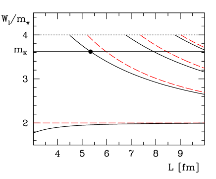
Figure 6: Two-pion energy spectrum in QCD below the inelastic threshold and as a function of the length of the box’s sides. The dashed curves correspond to free pions. The solid curves correspond to interacting pions in the $I=J=0$ channel. Also shown is the kaon mass, $m_{K}$, and the intersection of the first excited state ($\ell=1$) with this mass (dot).

The first thing to note is that the spectrum is far from continuous for any value of $L$ one may hope to reach in numerical simulation. The second point is that the corrections to the spectrum brought about by $\pi\pi$ interactions are not that large. This is due to the fact that they appear suppressed by $1/L^{3}$ and the volumes considered are not that small. A third point is that Eq. (29) can be turned around. Thus, a numerical study of the finite-volume two-pion spectrum can be converted into a determination of the phase shift $\delta_{0}^{I}(k)$ [58].

7.3 $K\to\pi\pi$ decays in finite volume

Having established that the two-pion levels are discrete, one can then imagine isolating $K$ decays to some of these excited two-pion levels, thus determining the matrix element 

$$M^{I}_{\ell}\equiv\langle(\pi\pi)_{I}\ell|\mathcal{H}_{\Delta S=1}|K\rangle\ .$$ (31)

In Eq. (31), all finite volume states are normalized to one: $\langle K|K\rangle=\langle(\pi\pi)_{I}\ell|(\pi\pi)_{I}\ell\rangle=1$.

Furthermore, having obtained $\delta_{0}^{I}(k)$ from a numerical study of the finite-volume two-pion spectrum, one can imagine tuning $L$ in such a way that the $n^{th}$ $\pi\pi$ state has energy $W_{n}=m_{K}$. This is illustrated by a dot in Figure 6, for $n=1$. The corresponding transition matrix element, $M^{I}_{n}$, conserves both energy and momentum and the kaons and pions have their physical masses. It is not, however, a finite-volume matrix element that we are after. What we want is the matrix element which describes the decay of a kaon at rest into a state of two asymptotic pions with energy $m_{K}$, i.e. $T^{I}_{n}\equiv\langle(\pi\pi\,out)_{I};m_{K}|\mathcal{H}_{\Delta S=1}|K\rangle$. The hard work enters in showing that these two matrix elements are related.

In [27], it is shown that the infinite-volume amplitude, $T^{I}_{n}$, is related to the corresponding finite-volume matrix element, $M^{I}_{n}$, through 

$$\left|T^{I}_{n}\right|^{2}=8\pi\,L^{6}\left\{q\,\phi^{\prime}(q)+k\,\delta_{0}^{I\prime}(k)\right\}_{k=k_{n}}$$ (32)

$$\times\left(\frac{m_{K}}{k_{n}}\right)^{3}\left|M^{I}_{n}\right|^{2}\ .$$

This result assumes that $W_{n}<4m_{\pi}$ and that the final two-pion state $|(\pi\pi)_{I}n\rangle$ is not degenerate (i.e. $n<8$). It is accurate up to exponentially small corrections in $L$.

There are various ways to proceed to prove this relation [27]. One approach is to study the normalization of $\pi\pi$ wavefunctions in finite and infinite volume, with the quantum-mechanical formalism of [58, 63]. Then one uses the fact that the transition matrix elements probe the $S$-wave component of the two-pion wavefunction near the origin and that this component differs in finite and infinite volume only in its normalization and possibly phase.

Instead, one can switch on the weak interaction ($\mathcal{H}_{\Delta S=1}$) and compute its influence on $\pi\pi$ energies. This can be done directly, using ordinary quantum-mechanical perturbation theory, or one may start from Eq. (29), taking into account the effect of the weak interaction on the scattering phase. A comparison of the two results yields the relation of Eq. (32).

One can also verify this relation by working out both finite and infinite-volume amplitudes in perturbation theory, in a low-energy effective theory such as $\chi$PT. Because Eq. (32) does not depend on the details of the dynamics of the system, a highly simplified model was chosen in [27], so as not to obscur the relation between the amplitudes, with complicated interactions and unnecessary quantum numbers. Since this calculation does not rely on Eq. (29), it can provide additional confidence in the correctness of Eq. (32) and illustrates how this relation plays out in the context of a relativistic field theory.

Recently, yet another derivation of Eq. (32) was proposed [28, 29]. The relation between this new approach and that of [27] should be clarified soon [28].

7.4 Application to the $\Delta I=1/2$ rule

Let $n=1$ with $W_{n}=m_{K}$. One possible statement of the $\Delta I=1/2$ rule is that $|T^{0}_{n}|/|T^{2}_{n}|\simeq 22$. What does this rule look like in finite volume?

For the purpose of illustration, we suppose that the scattering phases $\delta^{I}_{0}$ are accurately given by their one-loop expression in $\chi$PT [61].  Then, using the two-pion energy formulae of Eq. (29), the size of the box, $L$, required for the first excited state ($n=1$) to have energy $W_{1}$ equal to the kaon mass can be calculated in the two isospin channels. The results are shown in Table 2. Once the size of the boxes is fixed, it is straightforward to obtain the proportionality factor which appears in Eq. (32). The different contributions to this factor are also given in Table 2.

Table 2: Size of the box, $L$, required for the first excited, two-pion state to have energy equal to $m_{K}$ in the isopin 0 and 2 channels. Also given are the contributions to the proportionality factor which appears in Eq. (32).

$I$	$L\,[\mbox{fm}]$	$q$	$q\,\phi^{\prime}(q)$	$k\,\delta_{0}^{I\prime}(k)$
0	5.34	0.89	4.70	1.12
2	6.09	1.02	6.93	$-0.09$

One ends up with

$$|T^{0}_{n}|=44.9\times|M^{0}_{n}|,\qquad|T^{2}_{n}|=48.7\times|M^{2}_{n}|,$$ (33)

and

$$\left|T^{0}_{n}/T^{2}_{n}\right|=0.92\times\left|M^{0}_{n}/M^{2}_{n}\right|\ .$$ (34)

While the factors in Eq. (33) look large, they are mainly due to the relative normalization of free states in finite and infinite volume. Indeed, in the free case (i.e. with the scattering phases set to zero), the relation is $|T^{I}_{n}|=47.7\times|M^{I}_{n}|$. Thus, the effect of interactions is relatively small despite the large difference between the scattering phases in the two isospin channels (approximatively $45^{o}$ for $k=\sqrt{m_{k}^{2}/4-m_{\pi}^{2}}$). This means, in particular, that if QCD is to reproduce the $\Delta I=1/2$ enhancement, the large factor will have to come from the ratio of finite volume matrix elements, $\left|M^{0}_{n}/M^{2}_{n}\right|$. In fact, as Eq. (34) suggests, the effect should even be slightly larger in finite volume.

7.5 Summary

$K\to\pi\pi$ rates can, in principle, be obtained from the lattice without any model assumptions and without analytic continuation [27]. This requires working on lattices whose sides, $L$, are greater than $5\,\mbox{fm}$. On these lattices, the effect of interactions on the proportionality factor relating the transition matrix elements in finite and infinite volume was found to be small. This means that the finite-volume amplitudes must incorporate most of the physics which enters the determination of their infinite volume counterparts. In particular, if QCD is to reproduce the $\Delta I=1/2$ enhancement, this enhancement will be clearly visible in finite volume.

For the approach to be fully self-contained, the strong scattering phases, which are required to relate the finite and infinite volume amplitudes, should also be determined on the lattice. As shown by Lüscher many years ago [58, 63] and as briefly discussed above, this can again be done using finite-volume techniques. Here, the recent high-precision determination of $\pi\pi$, $S$-wave scattering lengths by Colangelo et al. [64] should provide a good test of some of the lattice techniques required to undertake such studies.

The same ideas as those described above can be applied to baryon decays, such as $\Lambda\to N\pi$, $\Sigma\to N\pi$ and $\Xi\to\Lambda\pi$, as well as to any other decay in which the final-state particles scatter only elastically.

There are, however, many potential hurdles in implementing the approach. It may be difficult, for instance, to extract excited $\pi\pi$ states in practice. Furthermore, since the unitarity of the underlying theory played an essential rôle in the argument leading to the relation of Eq. (32), it is not clear to what extent this relation holds in quenched QCD. Quenched $\chi$PT, along the lines of [65, 66], should help shed light on this problem. Finally, the approach taken here only applies to situations where the particles in the final state scatter elastically. It says very little about what should be done when they can scatter inelastically, as for example in $B\to\pi\pi$, $D\to K\pi$, $\ldots$ decays.

8 Conclusions

This has been an exciting year. New ideas for dealing with non-leptonic weak decays and for reducing operator mixing with Wilson fermions have been proposed.

There are new chiral perturbation theory results relevant for extracting $K\to\pi\pi$ amplitudes from $K\to\pi$ and $K\to 0$ matrix elements and from unphysical $K\to\pi\pi$ matrix elements.

There are also new numerical results, many of which are still preliminary, for:

• $\Delta S=2$ matrix elements relevant for $K^{0}$-$\bar{K}^{0}$ mixing in the standard model and beyond, with domain-wall and $\mathcal{O}\left(a\right)$-improved Wilson fermions;

• $K\to(\pi\pi)_{I}$ decays in the CP conserving and violating sectors, obtained from $K\to\pi$ and $K\to 0$ matrix elements, with domain-wall (for $I=0,2$) and $\mathcal{O}\left(a\right)$-improved Wilson (for $I=2$) fermions.

One thus expects, in the near future, lattice determinations of $\mathrm{Re}\;\epsilon^{\prime}/\epsilon$ and studies of the $\Delta I=1/2$-rule, hopefully with an active charm. In interpreting these results, when they come out, it will be important to keep in mind the difficulties of this calculation and the limitations of the $K\to\pi$ and $K\to 0$ approach, as discussed in Section 5.2.

There should also soon be results for $K\to(\pi\pi)_{I=2}$ decays in the CP conserving and violating sectors, from $K\to\pi\pi$ matrix elements, obtained with $\mathcal{O}\left(a\right)$-improved Wilson fermions. Kinematical situations other than the traditional $m_{K}=m_{\pi}$ with the two pions at rest will be investigated. It is further expected that these studies will be extended to $\Delta I=1/2$ transitions.

In any event, the coming year may yet be even more exciting.

Acknowledgements

I would like to thank S. Aoki, T. Blum, N. Christ, M. Golterman, M. Knecht, C.-J. D. Lin, M. Lüscher, G. Martinelli, R. Mawhinney, J.-I. Noaki, C. Sachrajda, A. Soni, Y. Taniguchi and M. Testa for sharing their results with me and/or for interesting discussions. I am grateful to David Lin for his careful reading of the manuscript. Many thanks to the organizers, also, for a delightful conference. Work supported in part by TMR, EC-Contract No. ERBFMRX-CT980169.

References

- [1]
- [2] A. Alavi-Harati et al., Phys. Rev. Lett. 83 (1999) 22.
- [3] V. Fanti et al., Phys. Lett. B465 (1999) 335.
- [4] Y. Taniguchi, these proceedings.
- [5] T. Blum, these proceedings.
- [6] A. Donini et al., Phys. Lett. B470 (1999) 233.
- [7] D. Becirevic et al. [SPQcdR Collaboration], hep-ph/0010349.
- [8] G. Martinelli, these proceedings.
- [9] A. Buras, hep-ph/9806471.
- [10] M. K. Gaillard and B. W. Lee, Phys. Rev. Lett. 33 (1974) 108.
- [11] G. Altarelli and L. Maiani, Phys. Lett. B52 (1974) 351.
- [12] C. Bernard et al., Phys. Rev. D32 (1985) 2343.
- [13] C. Bernard et al., Nucl. Phys. (PS) 4 (1988) 483.
- [14] M. Bochicchio et al., Nucl. Phys. B262 (1985) 331.
- [15] L. Maiani et al., Phys. Lett. B176 (1986) 445; Nucl. Phys. B289 (1987) 505.
- [16] G. Martinelli et al., Nucl. Phys. B445 (1995) 81.
- [17] K. Jansen et al., Phys. Lett. B372 (1996) 275.
- [18] C. Dawson et al., Nucl. Phys. B514 (1998) 313.
- [19] S. Sint, talk given at Workshop on Current Theoretical Problems in Lattice Field Theory, Ringberg, Germany, 2-8 April 2000.
- [20] D. Becirevic et al., Phys. Lett. B487 (2000) 74.
- [21] S. Aoki et al., Phys. Rev. D60 (1999) 114504.
- [22] S. Aoki and Y. Kuramashi, hep-lat/0007024.
- [23] C. Dawson, Nucl. Phys. (PS) 83 (2000) 854; these proceedings.
- [24] C. Alexandrou et al., Nucl. Phys. B580 (2000) 394.
- [25] S. Capitani and L. Giusti, Phys. Rev. D62 (2000) 114506.
- [26] L. Maiani and M. Testa, Phys. Lett. B245 (1990) 585.
- [27] L. Lellouch and M. Lüscher, hep-lat/0003023.
- [28] C.-J. D. Lin et al., in preparation.
- [29] M. Testa, hep-lat/0010020.
- [30] P. Vranas, these proceedings.
- [31] R. Edwards and U. Heller, hep-lat/0005002.
- [32] P. Hernández et al., hep-lat/0007015.
- [33] T. Blum et al., hep-lat/0007038.
- [34] A. Ali Khan et al. [CP-PACS Collaboration], hep-lat/0007014.
- [35] C. Jung et al., hep-lat/0007033.
- [36] R. Mawhinney, these proceedings.
- [37] S. Bertolini et al., hep-ph/0002234; J. Bijnens and J. Prades, hep-ph/0010008; J. Donoghue and E. Golowich, Phys. Lett. B478 (2000) 172; T. Hambye and P. Soldan, hep-ph/0009073; M. Knecht et al., Nucl. Phys. (PS) 86 (2000) 279.
- [38] V. Cirigliano and E. Golowich, Phys. Lett. B475 (2000) 351.
- [39] M. Golterman and E. Pallante, JHEP 0008 (2000) 023.
- [40] R. Frezzotti et al., Nucl. Phys. (PS) 83 (2000) 941.
- [41] T. Blum and A. Soni, Phys. Rev. Lett. 79 (1997) 3595.
- [42] S. Peris and E. de Rafael, Phys. Lett. B490 (2000) 213.
- [43] S. Aoki et al. [JLQCD Collaboration], Phys. Rev. Lett. 80 (1998) 5271.
- [44] G. Kilcup et al., Phys. Rev. D57 (1998) 1654.
- [45] G. Kilcup et al., Nucl. Phys. (PS) 53 (1997) 345.
- [46] G. Kilcup et al., Phys. Rev. Lett. 64 (1990) 25.
- [47] S. Aoki et al. [JLQCD Collaboration], Phys. Rev. D60 (1999) 034511.
- [48] L. Lellouch and C. J. Lin [UKQCD Collaboration], Nucl. Phys. (PS) 73 (1999) 312.
- [49] R. Gupta et al., Phys. Rev. D55 (1997) 4036.
- [50] S. Sharpe, hep-lat/9811006.
- [51] J. Noaki, these proceedings.
- [52] M. Gavela et al., Nucl. Phys. B306 (1988) 677.
- [53] C. Bernard and A. Soni, Nucl. Phys. (PS) 9 (1989) 155; ibid. 17 (1990) 495.
- [54] S. Aoki et al. [JLQCD Collaboration], Phys. Rev. D58 (1998) 054503.
- [55] Y. Kuramashi, Nucl. Phys. (PS) 83 (2000) 24.
- [56] N. G. Deshpande et al., Phys. Lett. B326 (1994) 307.
- [57] M. Ciuchini et al., Phys. Lett. B380 (1996) 353.
- [58] M. Lüscher, Nucl. Phys. B354 (1991) 531.
- [59] J. Gasser and H. Leutwyler, Phys. Lett. B125 (1983) 325; Annals Phys. 158 (1984) 142; Nucl. Phys. B250 (1985) 465.
- [60] J. Gasser and U. Meissner, Phys. Lett. B258 (1991) 219.
- [61] M. Knecht et al., Nucl. Phys. B457 (1995) 513.
- [62] M. Lüscher and U. Wolff, Nucl. Phys. B339 (1990) 222.
- [63] M. Lüscher, Comm. Math. Phys. 104 (1986) 177; Comm. Math. Phys. 105 (1986) 153.
- [64] G. Colangelo et al., Phys. Lett. B488 (2000) 261.
- [65] C. Bernard and M. Golterman, Phys. Rev. D53 (1996) 476.
- [66] M. Golterman and K. Leung, Phys. Rev. D56 (1997) 2950; ibid. D57 (1998) 5703; ibid. D58 (1998) 097503.