Non-equilibrium field theory

Abstract

I discuss various topics in relativistic non-equilibrium field theory related to high energy physics and cosmology. I focus on non-perturbative problems and how they can be treated on the lattice.

1 INTRODUCTION

The subject of non-equilibrium field theory is the evolution of many-particle systems in real (Minkowski) time. It also gives new insights into the much better understood equilibrium properties of quantum fields. Most of its applications in high energy physics are related to the early universe and to heavy ion collisions.

Many interesting problems in non-equilibrium field theory are non-perturbative. One could hope that they can be put on a lattice and then be solved by a computer. However, lattice simulations of quantum field theory (QFT) work in Euclidean time and nobody knows how to perform real time simulations.

A considerable simplification occurs for systems which are in partial (or incomplete) equilibrium (see, e.g., [1]). It means that some slowly relaxing quantities $y_{\alpha}$ differ significantly from their equilibrium values, while all other degrees of freedom are thermalized. The most extreme example are hydrodynamic modes, their relaxation times diverge when their wavelengths go to infinity (other examples will be discussed in Sec. 4). The non-equilibrium problem can then be reduced to evolution equations for the $y_{\alpha}$. These equations contain so called transport coefficients, and the task of non-equilibrium field theory is to determine them from the underlying QFT.

Partial equilibrium is a good approximation for most of the history of the early universe (an important exception is (p)reheating at the end of inflation, that is the transition to a radiation dominated epoch, see Sec. 2.1). Needless to say that the most solid results have been obtained for this case.

Fluctuation dissipation relations allow to express transport coefficients in terms of thermal averages like

$$\langle[O(t),O(0)]\rangle,$$ (1)

where the angular brackets denote the average over a thermal ensemble with temperature $T$,

$$\langle\cdots\rangle\equiv Z^{-1}{\rm tr}(\cdots e^{-H/T});$$ (2)

$H$ is the Hamiltonian. For example, electric conductivity is obtained from (1) with $O$ being the electromagnetic current (color conductivity, on the other hand, has no interpretation in terms of a gauge invariant correlation function of some current. Instead it arises as a “Wilson coefficient” in an effective theory for long distance modes of non-abelian gauge fields, see Sec. 4.2).

I have already mentioned that a serious difficulty of thermal field theory is the fact that one has to deal with real time. Let me illustrate this for the case of the expectation value (1). One could think of expanding Eq. (1) in powers of $t$. Then one can compute every coefficient in the expansion from the usual Euclidean path integral of thermal QFT. But transport coefficients are determined by the small frequency limit of the Fourier transform of (1). This depends on the behaviour for $t\to\infty$ which can not be captured by an expansion around $t=0$.

Fortunately there is a limit of quantum field theory in which a non-perturbative treatment is possible. It is the classical field limit of bosonic fields. It applies when the number of quanta in the field modes of interest is large. This is indeed the case in a variety of interesting problems. I discuss the classical field approximation, together with some recent applications in Sec. 2. A wide class of approximations, many of them related to a large $N$ expansion, which are not restricted to the classical field limit is discussed in Sec. 3. In Sec. 4 I consider systems in incomplete equilibrium. I show how one can use the classical field approximation even when quantum effects are important by constructing effective classical field theories. Sec. 5 is a brief summary of my talk.

2 CLASSICAL FIELD APPROXIMATION

While quantum systems are impossible to simulate in real time, there is no principle obstacle to performing real time simulations in classical field theory. All one has to do is to solve classical field equations of motion with the appropriate initial conditions, and determine the physical quantity of interest from the solution.

A well known special case of the classical field approximation (usually not referred to as such) is the dimensional reduction of a $d+1$ dimensional thermal QFT in the imaginary time formalism to the $d$ dimensional theory for the zero Matsubara frequency modes of the bosonic fields [2]. This is the formal classical limit because for $\hbar\to 0$ the non-zero modes become infinitely heavy and decouple. The thermodynamics of QFT can be studied with 4-dimensional lattice simulations, which is the only reliable way to access the properties of hot QCD near the critical temperature. Dimensional reduction is convenient for very high temperatures when there is a large separation of the scale $2\pi T$ and the screening length(s) of the system. In non-equilibrium field theory the role of the classical field approximation is much more important since there is no tractable analogue of the 4-dimensional Euclidean theory.

The classical field approximation should be reliable when the number of field quanta in each relevant field mode is large. There are indeed interesting applications where this is the case. The remainder of this section is a list of some of them.

2.1 Preheating after inflation

Inflation is the only known solution to the horizon and flatness problem in standard Big Bang cosmology. Furthermore, it generates density fluctuations which can seed the structure formation once electrons and nuclei have combined to form atoms. There has been a lot of interest in the transition from an inflationary to the radiation dominated epoch after it was realized [3] that the initially homogeneous inflaton field $\varphi$ can decay very rapidly into low momentum modes of the inflaton itself or into modes of other scalar fields $\chi$ through parametric resonance. This mechanism is referred to as pre-heating, and it has drastically changed the picture of reheating after inflation.

The large amplitudes of the amplified modes make this problem non-perturbative. At the same time, the occupation numbers of these modes grow very large which opens the possibility to study this problem in the classical field approximation on the lattice [4, 5]. As an illustration, Fig. 1 shows the occupation number of the $\chi$ field (taken from Ref. [6]).

Lattice simulations have shown that non-linear effects play an important role in reheating [5, 6]. Effects like non-thermal phase transitions and defect formation have been investigated [7, 8, 9, 10]. Preheating and the possibility of non-thermal phase transitions in gauge theories were studied in [11].

Figure 1: Occupation numbers of $\chi$-modes vs momentum. The curves correspond to different values of time. There are three visible resonances caused by the oscillating inflaton background (from Ref. [6]).

2.2 Small $x$ gluon distributions

The gluon density in hadrons and nuclei becomes large at small $x$, where $x$ is the fraction of the momentum of the hadron/nucleus which is carried by the gluon. Then the usual perturbative treatment of parton evolution breaks down. In [12] a model was proposed which describes the small $x$ gluon field of large nuclei classically. It was first applied to nuclear collisions in Ref. [13]. If one is interested in the production of gluons with small transverse momenta a non-perturbative treatment of this model is necessary. A lattice version was developed in [14]. It was used to solve the non-linear equations of motion for the gluon fields of two colliding nuclei, and energy densities and gluon multiplicities in the final state were extracted [15].

2.3 Tests of approximation schemes

The approximation schemes to be discussed in Sec. 3 are usually formulated in quantum field theory. It is difficult to asses their reliability. In Ref. [16] it was pointed out that they can equally well be formulated in the classical field limit. It is then possible to perform lattice simulations and compare the “exact” lattice results with the approximate ones. For a scalar model in (1+1) dimensions it was found that early-time behaviour is reproduced qualitatively by the Hartree approximation, and that including scattering improves this to the quantitative level. At late times the lattice system thermalizes, but the improved Hartree approximation fails to reproduce this behaviour [17].

2.4 Droplet nucleation in a thermal first order phase transition

Starting from a high temperature, a first order phase transition proceeds through the nucleation of droplets, which then grow and eventually fill the whole space with the low temperature phase. The droplet nucleation is caused by thermal fluctuations. Most calculations of the nucleation rate use the formalism due to Langer [18] which is based on a saddle point approximation around the the critical droplet. A lot of lattice computations have been performed, most of them have considered a moderately strong first order phase transition (for recent results, see [19]). Ref. [20] has considered a very strongly first order transition in the electroweak theory. The results were compared with various analytic calculations based on Langer’s approach. It was found that the accuracy of the analytic results strongly depend on the approximation used for the critical droplet action. The best agreement was found when the 2-loop effective potential for the Higgs field [21, 22] together with the field dependent wave function renormalization [23, 24] is used.

3 BEYOND THE CLASSICAL FIELD APPROXIMATION

The classical field approximation is clearly restrictive, and it is not capable of treating genuine quantum effects. For example, the thermalization of the universe after preheating (cf. Sec. 4) is not classical. It is sometimes possible to obtain effective classical theories when the non-classical modes are weakly interacting and can be integrated out in perturbation theory (see Sec. 4.2). In general, however, other approximations are necessary.

The Hartree approximation was discussed in the talk by J. Vink [25] and there are several related approaches. Usually the basic idea is to work directly with non-equilibrium Green functions or, alternatively, with the generating functional of 1-PI Green functions [26]. These satisfy certain Schwinger-Dyson-like equations which are an infinite set of equations containing the full set of $n$-point functions. To make this problem tractable, the hierarchy of Schwinger-Dyson equations must be truncated. It is possible to formulate such truncations as a systematic expansion in $1/N$, where $N$ is the number of some fields [27, 28].

Recent lattice studies have focused on the question whether one can obtain thermalization staring from some non-equilibrium initial state (see also Sec. 2.3). Thermalization can be obtained in the Hartree approximation if the mean field is allowed to be inhomogeneous, which was discussed in J. Vink’s talk [25]. Thermalization of fermionic modes, which can never be described by classical fields, was also observed in the inhomogeneous mean field approximation [29].

Ref. [30] considers (1+1) dimensional $\lambda\varphi^{4}$ theory in the loop expansion of the generating functional of 2-particle irreducible non-equilibrium Green functions. At 3-loop order, when scattering is taken into account, thermalization was observed.

4 CLOSE TO THERMAL EQUILIBRIUM

As I mentioned in the introduction, there are interesting non-equilibrium processes in which most of the degrees of freedom are equilibrated and only some slowly relaxing ones are not. The task of non-equilibrium field theory is then to determine the relevant diffusion coefficients.

In weakly coupled theories it is possible to compute some transport coefficients using perturbation theory. This is not an easy task. Typically one has to sum an infinite set of diagrams, which was done for the shear and bulk viscosity in (3+1) dimensional scalar theory with cubic and quartic self interactions [31]. The result of [31] is equivalent to the solution of the classical Boltzmann equation with appropriate coefficients. Other transport coefficients were calculated starting directly from the Boltzmann equation, which is technically much simpler than a diagrammatic analysis [32]. Another application of the Boltzmann equation of current interest is the generation of a lepton asymmetry due to heavy Majorana neutrinos [33].

Unfortunately, it is not clear whether the classical Boltzmann equation is the leading order effective theory in some systematic weak coupling expansion which would allow to go beyond the leading order. There are problems where this is necessary, like for example in electroweak baryogenesis [34].

There are transport coefficients which are not computable in (appropriately resummed) perturbation theory even when the coupling constant is small. A famous example is the rate $\gamma_{B+L}$ for baryon ($B$) plus lepton number ($L$) dissipation in the standard electroweak theory [34]. The Lagrangian of the electroweak theory has a U(1) symmetry which would imply that $B+L$ is conserved. However, this symmetry is anomalous, and $B+L$ violating processes are possible. Suppose there is some non-zero density $N_{B+L}$ in the universe. It then gets washed out according to

$$\frac{d}{dt}N_{B+L}=-\gamma_{B+L}N_{B+L}.$$ (3)

There is a fluctuation dissipation relation stating that $\gamma_{B+L}$ is proportional to the Chern-Simons diffusion rate $\Gamma_{\rm CS}$ of the weak SU(2) gauge fields. $\Gamma_{\rm CS}$ is dominated by soft gauge field modes with typical momenta of order $g^{2}T$. This is the so called magnetic screening scale at which perturbation theory for hot Yang-Mills theory breaks down [35]. Fortunately the smallness of this scale allows the use of the classical field approximation to compute $\Gamma_{\rm CS}$. The occupation number of the bosonic field modes can be estimated from the Bose-Einstein distribution function

$$n({\bf k})=\frac{1}{e^{|{\bf k}|/T}-1}\simeq\frac{T}{|{\bf k}|}\quad(|{\bf k}|\ll T)$$ (4)

which is of order $1/g^{2}$ for the soft ($|{\bf k}|\sim g^{2}T$) modes.

The question how to calculate $\Gamma_{\rm CS}$ has a long history. One reason for this long lasting interest is that the $B+L$ dissipation rate is a fundamental quantity of the Standard Model of electroweak interactions (SM) and extensions thereof. It plays an important role in particle physics scenarios for generating the baryon asymmetry of the universe. The use of classical lattice field theory for calculating $\Gamma_{\rm CS}$ was first suggested in Ref. [36], where a (1+1) dimensional model was studied.

Originally it was assumed that the naive classical field approximation correctly describes the dynamics of the soft modes in (3+1) dimensional Yang-Mills theory. Therefore the lattice version of the classical Yang-Mills equations of motion

$$D_{0}{\bf E}+{\bf D}\times{\bf B} = 0,$$ (5.a)

$${\bf D}\cdot{\bf E} = 0,$$ (5.b)

were solved and used to determine the Chern-Simons diffusion [38, 39, 40] (see also [47]). Here ${\bf E}$ and ${\bf B}$ are the color electric and magnetic fields and $D_{\mu}$ denotes the covariant derivative $\partial_{\mu}+gA_{\mu}$ in the adjoint representation. The above assumption would be correct if high momentum ($|{\bf k}|\gg g^{2}T$) modes decouple from the soft dynamics. It is suggestive because it is true for the thermodynamics of hot Yang-Mills fields: At leading order in $g$ the soft non-perturbative modes are described by the 3-dimensional pure Yang–Mills theory of dimensional reduction, and the only role of high momentum modes is to make the coupling constant equal to its renormalized value.

4.1 Problems of the classical field approximation

Classical thermal field theory as a continuum theory does not exist. This has been known for more than 100 years and it has played a crucial role in the discovery of quantum theory by Planck.

In dimensional reduction the UV divergences are taken care of by adding the appropriate local counterterms to the 3-dimensional action. Then long distance ($l\gg T^{-1}$) correlation functions of the 4-dimensional theory are correctly reproduced by the 3-dimensional one.

However, it was realized in [41] that there are UV divergences in classical thermal Yang-Mills theory which do not occur in equal time correlation functions . These divergences are closely related to what is called “hard thermal loops” in thermal QFT [52]. They are particularly ugly, they are non-local in space and time and on the lattice they are sensitive to the lattice geometry (see also [43]). The occurrence of such divergences in lattice field theory is possible due to the lack of Lorentz invariance which is explicitly broken by the presence of the thermal bath. As a consequence, Green functions with external momenta $p_{\alpha}$ depend not only on the Lorentz invariants $p_{\alpha}\cdot p_{\beta}$ but on frequencies and spatial momenta separately.

       

Figure 2: One-loop polarization tensor in non-abelian gauge theory. Only the first two diagrams contribute to the UV divergence in the classical field limit, while the ghost loop contribution is suppressed.

Since such divergences are probably not familiar to most of the audience, let me describe them in some more detail. They are due to the one-loop polarization tensor (see Fig. 2). First consider the case that the external momentum $k$ is purely spatial, $k_{0}=0$. This is what one encounters in the 3-dimensional reduced theory. The result is of the form

$$\Pi^{\mu\nu}(0,{\bf k})\sim g^{2}T\int^{\Lambda}\frac{d^{3}q}{{\bf q}^{2}}f\left(\frac{{\bf k}\cdot{\bf q}}{{\bf q}^{2}},\frac{{\bf k}^{2}}{{\bf q}^{2}}\right)$$ (6)

where the function $f$ is dimensionless, and $\Lambda$ is the UV cutoff. $f$ can be expanded in powers of its arguments, and only the lowest order term $f(0,0)$ gives rise to a linearly divergent integral,

$$\Pi^{\mu\nu}(0,{\bf k})\sim g^{2}T\Lambda f(0,0)+\mbox{UV finite}.$$ (7)

Gauge invariance ensures that this divergence occurs only in $\Pi^{00}$. This is nothing but the familiar divergence of the mass term for the adjoint Higgs field $A_{0}$ which is taken care of by adding a mass counterterm to the 3-dimensional action.

Now consider the analogous contribution when the external frequency is non-zero. In the classical field limit the result for $\Pi^{\mu\nu}$ is similar to Eq. (6). However, the function $f$ now depends on three dimensionless variables,

$$\Pi^{\mu\nu}(k)\sim g^{2}T\int^{\Lambda}\frac{d^{3}q}{{\bf q}^{2}}f\left(\frac{k^{0}}{\hat{{\bf q}}\cdot{\bf k}},\frac{{\bf k}\cdot{\bf q}}{{\bf q}^{2}},\frac{{\bf k}^{2}}{{\bf q}^{2}}\right).$$ (8)

To extract the divergent contribution one can again expand in powers of ${\bf k}\cdot{\bf q}/{\bf q}^{2}$ and ${\bf k}^{2}/{\bf q}^{2}$, but the dependence on the first argument of $f$ remains. Therefore the linearly divergent part of $\Pi^{\mu\nu}$ has a non-trivial dependence on $k^{0}/\hat{{\bf q}}\cdot{\bf k}$,

$$\Pi^{\mu\nu}(k)\sim g^{2}T\Lambda\int_{\hat{{\bf q}}}f\left(\frac{k^{0}}{\hat{{\bf q}}\cdot{\bf k}},0,0\right)+\mbox{UV finite}.$$ (9)

(I’ve been somewhat sketchy, for the precise form of the divergent contribution on the lattice see [41, 43].) Such a divergence is clearly a disaster because it is non-local in space and time. Effects of these divergences in lattice simulations have first been observed in Refs. [44, 45].

It was argued in [46] that the UV divergent part of $\Pi^{\mu\nu}$ has the same qualitative effect as the hard modes in the quantum theory (see Sec. 4.2), which is that it slows down the dynamics of the soft gauge field modes. In the continuum limit $\Lambda\to\infty$ the characteristic time scale of the soft modes should diverge, so that the Chern-Simons diffusion rate $\Gamma_{\rm CS}$ should go to zero. This behaviour was indeed observed in a recent calculation on a very fine lattice [47].

4.2 Effective classical theories

If the high momentum modes, which do not have large occupation numbers and are thus not classical, are so important for the soft field dynamics, can one still make use of the classical field approximation? This is indeed possible. The modes with momenta larger than $g^{2}T$ are weakly coupled and can be integrated out using perturbation theory. One finds that the correct effective classical theory, at leading order in $g$ and $\log(1/g)$, is described by the equation of motion [48]

$${\bf D}\times{\bf B}=\gamma{\bf E}+\mbox{\boldmath$\zeta$}$$ (10)

instead of Eq. (4). The constant $\gamma$ is proportional to $T/\log(1/g)$. Furthermore, $\zeta$ is a Gaussian white noise. Its expectation value vanishes and it is entirely determined by its 2-point function

$$\langle\zeta_{i}^{a}(x)\zeta_{j}^{b}(x^{\prime})\rangle=2T\gamma\delta^{ab}\delta_{ij}\delta^{(4)}(x-x^{\prime}).$$ (11)

Here $a$, $b$ are indices of the adjoint representation of the gauge group. Recently the leading log effective theory (10) was extended to include the Higgs field [49].

The physics behind Eq. (10) is easily understood. The soft gauge fields evolve in time, which means that the color electric field is non-zero. The hot plasma is a conductor and the electric field induces a current which is carried by charged particles corresponding to the hard (${\bf k}\sim T$) field modes. The particles suffer collisions with a typical mean free path of order $(\log(1/g)g^{2}T)^{-1}$. In the weak coupling limit $\log(1/g)\gg 1$ this is small compared to the wavelengths of the soft non-perturbative modes. Thus the soft modes cannot resolve the trajectories of the particles and the induced current is simply a number times the electric field. The noise term is due to thermal fluctuations of the field modes which have been integrated out.

Eq. (10) is similar to the equation of motion of an ordinary (abelian) magnetic field in a conducting plasma, where the role of $\gamma$ is played by the electric conductivity. (In analogy with electrodynamics one calls the coefficient in Eq. (10) color conductivity). The key difference is that the electrodynamics analogue of Eq. (10) is valid to arbitrary accuracy if one considers fields with longer and longer wavelengths. This is possible because abelian magnetic fields are not screened. On the other hand, non-abelian magnetic fields are screened on a length scale of order $(g^{2}T)^{-1}$. Thus there is nothing like a magneto-hydrodynamic limit in hot non-abelian plasmas. In fact, Eq. (10) is only valid at leading and, as was shown recently in Ref. [51], at next-to-leading order in $\log(1/g)^{-1}$.

From Eq. (10) one can estimate the characteristic frequency $k_{0}$ of the soft modes as follows. The rhs is of order $(g^{2}T)^{2}{\bf A}$, since it contains two covariant derivatives of the vector potential ${\bf A}$. The electric field which contains one time derivative can be estimated as $k_{0}{\bf A}$. Thus the characteristic frequency is

$$k_{0}\sim\log(1/g)g^{4}T.$$ (12)

This is much smaller than the estimate $k_{0}\sim g^{2}T$ which one would obtain assuming that high momentum modes decouple from the soft dynamics. From Eq. (12) one can estimate the Chern-Simons diffusion rate, which is the number of topological transitions per unit time and unit volume, as

$$\Gamma_{\rm CS}\sim k_{0}|{\bf k}|^{3}\sim\log(1/g)\alpha^{5}T^{4},$$ (13)

where $\alpha=g^{2}/(4\pi)$.

Eq. (12) was obtained through a sequence of effective field theories by integrating out more and more high momentum degrees of freedom. The first is the so called

Hard thermal loop effective theory
It is the result of integrating out “hard” physics associated with $k^{2}$ of order $T^{2}$, and it can be described by the classical field equations of motion [53]

$$D_{0}{\bf E}+{\bf D}\times{\bf B} = m^{2}_{\rm D}{\bf W}$$ (14.a)

$${\bf D}\cdot{\bf E} = m^{2}_{\rm D}W^{0}$$ (14.b)

$$v\cdot DW = {\bf v}\cdot{\bf E}.$$ (14.c)

The field $W=W(x,{\bf v})$ represents the fluctuations of adjoint color charge due to the hard degrees of freedom, which act like particles with 3-velocity ${\bf v}$, ${\bf v}^{2}=1$. Furthermore,

$$v^{\mu}=(1,{\bf v}).$$ (15)

The 4-current on the rhs of Eqs. (14.a) and (14.b) is given by

$$W^{\mu}(x)=\int\frac{d^{2}\Omega_{{\bf v}}}{4\pi}v^{\mu}W(x,{\bf v}),$$ (16)

times the square of the leading order Debye mass $m_{\rm D}\propto gT$. Originally hard thermal loops where discovered when trying to develop a consistent perturbative expansion of Greens functions with external momenta of order $gT$ [52]. The effect of hard thermal loops on the soft dynamics was first realized in Ref. [46] where the fields in Eq. (4.2) where interpreted as being soft. Then the main effect of the hard particles is Landau damping [54] of the soft modes, resulting in the estimate $k_{0}\sim g^{4}T$, which is the same as Eq. (12) but without the logarithm. It was then realized that the fields in Eq. (4.2) must be interpreted as modes with both ${\bf k}\sim gT$ and ${\bf k}\sim g^{2}T$ [48].

Non-abelian Boltzmann equation
The ${\bf k}\sim gT$ modes in Eq. (4.2) are weakly coupled and can be integrated out in an expansion in $g$. They are responsible for small angle scattering between the hard particles. They induce a collision term and noise term in Eq. (14.c), and one obtains [48]

$$D_{0}{\bf E}+{\bf D}\times{\bf B} = m^{2}_{\rm D}{\bf W}$$ (17.a)

$${\bf D}\cdot{\bf E} = m^{2}_{\rm D}W^{0}$$ (17.b)

$$(C+v\cdot D)W = {\bf v}\cdot{\bf E}+\xi,$$ (17.c)

where now the gauge and $W$ fields contain only spatial Fourier components of order $g^{2}T$ (modulo logarithms of $1/g$). The linear collision term $CW$ breaks time reflection invariance and describes dissipation caused by the modes which have been integrated out. These modes also perform thermal fluctuations which pump energy back into the $g^{2}T$ modes through the Gaussian white noise $\xi$. (For other approaches, which do not make use of the hard thermal loop effective theory, see Refs. [55, 56, 57, 58].)

Langevin equation(s)
The collision term $C$ in Eq. (17.c) is of order $\log(1/g)g^{2}T$, while derivatives of the non-perturbative modes are of order $g^{2}T$. At leading order in $\log(1/g)^{-1}$ the latter can be neglected. Then the current on the rhs of Eq. (17.a) is a local and linear function of ${\bf E}$ and $\xi$. Due to the strong damping one can neglect the kinetic term $D_{0}{\bf E}$ in Eq. (17.a) which leads to Eq. (10).

Starting from a non-local Langevin equation which is valid to all order in $\log(1/g)^{-1}$ [50] it was shown that the logarithmic approximation can be systematically improved in an expansion in $\log(1/g)^{-1}$ [51]. It was found that Eq. (10) is still valid at next-to-leading order in $\log(1/g)^{-1}$ if one includes a next-to-leading log correction in the color conductivity $\gamma$, which was computed in [51].

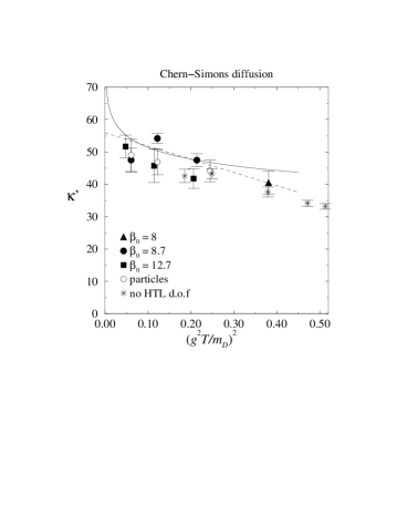
Figure 3: Chern-Simons diffusion rate parametrised by $\kappa^{\prime}$ (see Eq. (18)) vs the magnetic screening scale over Debye mass (for details see text).

4.3 Lattice results

The effective theory (10) is perfectly suited for lattice simulations because it is UV finite [55]. It was used to calculate the Chern-Simons diffusion rate in Ref. [59]. Due to Eq. (13) the result can be parametrized as

$$\Gamma_{\rm CS}=\kappa^{\prime}\frac{g^{2}T^{2}}{m^{2}_{\rm D}}\alpha^{5}T^{4}$$ (18)

with

$$\kappa^{\prime}=\kappa\log\left(\frac{m^{2}_{\rm D}}{g^{2}T}\right).$$ (19)

The dimensionless constant $\kappa$ was determined as

$$\kappa=10.8\pm 0.7.$$ (20)

Near a weakly first order electroweak phase transition one has to take into account the Higgs field which requires an extension of Eq. (10) [49], the resulting effect on $\Gamma_{\rm CS}$ is of order 20%.

The hard thermal loop effective theory (4.2) is a classical field theory which correctly incorporates the effect of the hard modes. Unlike the Langevin equation (10) its validity is not restricted to the logarithmic approximation, but it does not have a continuum limit. It was argued that it should still be useful for lattice simulations as long as the lattice spacing is not too small [60].

Two different lattice implementations of the hard thermal loop effective theory have been developed. In Ref. [61] the hard modes are represented by classical charged particles. This method was further developed and used to compute $\Gamma_{\rm CS}$ in Ref. [60]. Starting point of Ref. [62] were the equations of motion (4.2). The $W$ fields were expanded in spherical harmonics and only components $W_{lm}$ with $l$ smaller or equal to some cutoff $l_{\rm max}$ were kept.

The results are shown in Fig. 3. The rate $\Gamma_{\rm CS}$ is parametrized by $\kappa^{\prime}$ through Eq. (18). The black symbols are the results of Ref. [62] for 3 different values of the lattice spacing $a$, where

$$\beta_{0}\equiv\frac{4}{g^{2}Ta}.$$ (21)

The open circles are the results of Ref. [60]. Also shown are the results of Ref. [47] for the classical Yang-Mills theory (4). The different methods give surprisingly similar results. The dashed line is a linear fit $\kappa^{\prime}=c_{1}+c_{2}\left(\frac{g^{2}T}{m_{\rm D}}\right)^{2}$. The full line is a fit which includes the leading log term, $\kappa^{\prime}=\kappa\log\left(\frac{m^{2}_{\rm D}}{g^{2}T}\right)+c$.

The results shown in Fig. 3 are about a factor 5 larger than the leading log result. However, including the next-to-leading log correction to the color conductivity $\gamma$ increases the value of $\kappa^{\prime}$ in Eq. (19) by about a factor 5 [51], which gives a remarkable agreement with the results in Fig. 3.

5 SUMMARY

At present we see an interesting interplay between analytic and numerical lattice work on non-equilibrium field theory. It is motivated by the physics of the early universe and of heavy ion collisions. Real time simulations of non-equilibrium quantum field theory are not possible. A common tool is the classical field approximation which can be applied if the field modes of interest have large occupation numbers. There are several approaches which go beyond the classical field approximation. They require other approximations, such as Hartree-Fock, large $N$. It is possible to use the classical field approximation even when quantum effects are important by constructing effective classical theories. These can differ substantially from the naive classical limit of the underlying quantum field theory.

References

- [1] L. D. Landau, E. M. Lifshitz, Statistical Mechanics (Pergamon Press, Oxford).
- [2] See O. Philipsen, these proceedings, hep-lat/0011019; for reviews of high temperature dimensional reduction see, e.g., M. E. Shaposhnikov, hep-ph/9610247; A. Nieto, Int. J. Mod. Phys. A12, 1431 (1997) [hep-ph/9612291]; M. Laine, hep-ph/9707415, hep-ph/0010275.
- [3] L. Kofman, A. Linde and A. A. Starobinsky, Phys. Rev. Lett. 73, 3195 (1994) [hep-th/9405187].
- [4] D. T. Son, hep-ph/9601377.
- [5] S. Y. Khlebnikov and I. I. Tkachev, Phys. Rev. Lett. 77, 219 (1996) [hep-ph/9603378].
- [6] T. Prokopec and T. G. Roos, Phys. Rev. D55, 3768 (1997) [hep-ph/9610400].
- [7] S. Kasuya and M. Kawasaki, Phys. Rev. D56, 7597 (1997) [hep-ph/9703354].
- [8] S. Khlebnikov, L. Kofman, A. Linde and I. Tkachev, Phys. Rev. Lett. 81, 2012 (1998) [hep-ph/9804425].
- [9] S. Kasuya and M. Kawasaki, Phys. Rev. D58, 083516 (1998) [hep-ph/9804429].
- [10] G. Felder, L. Kofman, A. Linde and I. Tkachev, JHEP 0008, 010 (2000) [hep-ph/0004024].
- [11] A. Rajantie and E. J. Copeland, Phys. Rev. Lett. 85, 916 (2000) [hep-ph/0003025].
- [12] L. McLerran and R. Venugopalan, Phys. Rev. D49, 2233 (1994) [hep-ph/9309289]; Phys. Rev. D49, 3352 (1994) [hep-ph/9311205].
- [13] A. Kovner, L. McLerran and H. Weigert, Phys. Rev. D52, 3809 (1995) [hep-ph/9505320].
- [14] A. Krasnitz and R. Venugopalan, Nucl. Phys. B557, 237 (1999) [hep-ph/9809433].
- [15] A. Krasnitz and R. Venugopalan, Phys. Rev. Lett. 84, 4309 (2000) [hep-ph/9909203]; hep-ph/0007108.
- [16] G. Aarts, G. F. Bonini and C. Wetterich, Nucl. Phys. B587, 403 (2000) [hep-ph/0003262].
- [17] G. Aarts, G. F. Bonini and C. Wetterich, hep-ph/0007357.
- [18] J. S. Langer, Annals Phys. 41, 108 (1967).
- [19] S. Borsanyi, A. Patkos, J. Polonyi and Z. Szep, Phys. Rev. D62, 085013 (2000) [hep-th/0004059].
- [20] G. D. Moore and K. Rummukainen, hep-ph/0009132.
- [21] P. Arnold and O. Espinosa, Phys. Rev. D47, 3546 (1993) [hep-ph/9212235].
- [22] Z. Fodor and A. Hebecker, Nucl. Phys. B432, 127 (1994) [hep-ph/9403219].
- [23] D. Bödeker, W. Buchmüller, Z. Fodor and T. Helbig, Nucl. Phys. B423, 171 (1994) [hep-ph/9311346].
- [24] J. Kripfganz, A. Laser and M. G. Schmidt, Z. Phys. C73, 353 (1997) [hep-ph/9512340].
- [25] M. Salle, J. Smit and J. C. Vink, these proceedings, hep-lat/0010054.
- [26] C. Wetterich, Phys. Rev. Lett. 78, 3598 (1997) [hep-th/9612206].
- [27] F. Cooper, S. Habib, Y. Kluger, E. Mottola, J. P. Paz and P. R. Anderson, Phys. Rev. D50, 2848 (1994) [hep-ph/9405352].
- [28] D. Boyanovsky and H. J. de Vega, Phys. Rev. D61, 105014 (2000) [hep-ph/9911521].
- [29] G. Aarts and J. Smit, Phys. Rev. D61, 025002 (2000) [hep-ph/9906538].
- [30] J. Berges and J. Cox, hep-ph/0006160.
- [31] S. Jeon Phys. Rev. D 52 (1995) 3591; see also S. Jeon and L. G. Yaffe, Phys. Rev. D53, 5799 (1996) [hep-ph/9512263]; E. Wang and U. Heinz, Phys. Lett. B471, 208 (1999) [hep-ph/9910367].
- [32] For recent results, see P. Arnold, G. D. Moore and L. G. Yaffe, JHEP 0011, 001 (2000) [hep-ph/0010177].
- [33] W. Buchmüller and M. Plümacher, hep-ph/0007176.
- [34] For reviews of electroweak baryon number violation and electroweak baryogenesis, see A.G. Cohen, D.B. Kaplan, A.E. Nelson, Ann.Rev.Nucl.Part.Sci.43 (1993) 27 [hep-ph/9302210]; V.A. Rubakov, M. E. Shaposhnikov, Usp. Fis. Nauk 166 (1996) 493 [hep-ph/9603208]; A. Riotto and M. Trodden, Ann. Rev. Nucl. Part. Sci. 49, 35 (1999) [hep-ph/9901362].
- [35] A. D. Linde, Phys. Lett. B 96 (1980) 289; D. J. Gross, R. D. Pisarski and L. G. Yaffe, Rev. Mod. Phys. 53 (1981) 43.
- [36] D. Y. Grigoriev and V. A. Rubakov, Nucl. Phys. B299, 67 (1988); the (1+1) dimensional Abelian Higgs model was further studied in [37].
- [37] D. Y. Grigoriev, V. A. Rubakov and M. E. Shaposhnikov, Phys. Lett. B216, 172 (1989); A. I. Bochkarev and P. de Forcrand, Phys. Rev. D44, 519 (1991).
- [38] J. Ambjørn, T. Askgaard, H. Porter and M. E. Shaposhnikov, Phys. Lett. B244, 479 (1990); Nucl. Phys. B353, 346 (1991).
- [39] J. Ambjorn and A. Krasnitz, Phys. Lett. B362, 97 (1995) [hep-ph/9508202]; Nucl. Phys. B506, 387 (1997) [hep-ph/9705380].
- [40] W. Tang and J. Smit, Nucl. Phys. B482, 265 (1996) [hep-lat/9605016].
- [41] D. Bödeker, L. McLerran and A. Smilga, Phys. Rev. D52, 4675 (1995) [hep-th/9504123].
- [42] G. Aarts and J. Smit, Phys. Lett. B393, 395 (1997) [hep-ph/9610415].
- [43] P. Arnold, Phys. Rev. D55, 7781 (1997) [hep-ph/9701393].
- [44] D. Bödeker and M. Laine, Phys. Lett. B416, 169 (1998) [hep-ph/9707489].
- [45] W. H. Tang and J. Smit, Nucl. Phys. B510, 401 (1998) [hep-lat/9702017].
- [46] P. Arnold, D. Son and L. G. Yaffe, Phys. Rev. D55, 6264 (1997) [hep-ph/9609481]; P. Huet and D. T. Son, Phys. Lett. B393, 94 (1997) [hep-ph/9610259].
- [47] G. D. Moore and K. Rummukainen, Phys. Rev. D61, 105008 (2000) [hep-ph/9906259].
- [48] D. Bödeker, Phys. Lett. B426, 351 (1998) [hep-ph/9801430]; Nucl. Phys. B559, 502 (1999) [hep-ph/9905239]; Nucl. Phys. B566, 402 (2000) [hep-ph/9903478].
- [49] G. D. Moore, Phys. Rev. D62, 085011 (2000) [hep-ph/0001216].
- [50] P. Arnold, Phys. Rev. D62, 036003 (2000) [hep-ph/9912307].
- [51] P. Arnold and L. G. Yaffe, UW/PT 99-24, hep-ph/9912306; UW-PT-99-25, hep-ph/9912305.
- [52] E. Braaten and R. Pisarski, Nucl. Phys. B 337 (1990) 569; Phys. Rev. D 45 (1992) 1827; J. Frenkel and J.C. Taylor, Nucl. Phys. B 334 (1990) 199; J.C. Taylor and S.M.H. Wong, Nucl. Phys. B 346 (1990) 115.
- [53] J. P. Blaizot, E. Iancu, Nucl.Phys. B 417 (1994) 608. “Soft collective excitations in hot gauge theories,” Nucl. Phys. B417, 608 (1994) [hep-ph/9306294]; V.P. Nair, Phys. Rev. D48, 3432 (1993) [hep-ph/9307326].
- [54] E.M. Lifshitz, L.P. Pitaevskii, Physical Kinetics (Pergamon Press, Oxford 1981).
- [55] P. Arnold, D. T. Son and L. G. Yaffe, Phys. Rev. D59, 105020 (1999) [hep-ph/9810216].
- [56] M. A. Valle Basagoiti, hep-ph/9903462.
- [57] D. F. Litim and C. Manuel, Phys. Rev. Lett. 82, 4981 (1999) [hep-ph/9902430].
- [58] J. Blaizot and E. Iancu, Nucl. Phys. B557, 183 (1999) [hep-ph/9903389].
- [59] G. D. Moore, Nucl. Phys. B568, 367 (2000) [hep-ph/9810313].
- [60] G.D. Moore, C. Hu and B. Müller, Phys. Rev. D58, 045001 (1998) [hep-ph/9710436].
- [61] C. R. Hu and B. Müller, Phys. Lett. B409, 377 (1997) [hep-ph/9611292].
- [62] D. Bödeker, G.D. Moore, K. Rummukainen, Phys. Rev. D61, 056003 (2000) [hep-ph/9907545].