Heavy quark physics on the lattice

Abstract

I review the current status of lattice calculations of the properties of bound states containing one or more heavy quarks. Many of my remarks focus on the heavy-light leptonic decay constants, such as $f_{B}$, for which the systematic errors have by now been quite well studied. I also discuss $B$-parameters, semileptonic form factors, and the heavy-light and heavy-heavy spectra. Some of my “world averages” are: $f_{B}=200(30)\;{\rm Me\!V}$, $f_{B}\sqrt{\hat{B}_{B_{d}}}=230(40)\;{\rm Me\!V}$, $f_{B_{s}}/f_{B}=1.16(4)$ and $f_{B_{s}}\sqrt{\hat{B}_{B_{s}}}/f_{B}\sqrt{\hat{B}_{B_{d}}}=1.16(5)$.

1 INTRODUCTION

Many of the parameters of the Standard Model can be constrained by measurements of the properties of hadrons containing heavy quarks. To take advantage of such experiments, however, one needs theoretical determinations of the corresponding strong-interaction matrix elements. Lattice gauge theory provides, at least in principle, a means of computing hadronic matrix elements with control over all sources of systematic error. Here, I review the current status of these computations.

A review like this is necessarily somewhat idiosyncratic in the topics it covers and the time spent on each. I devote a large fraction of my time to $f_{B}$. Because lattice data for leptonic decay constants is more extensive than for any other heavy quark quantity, I am able to discuss in detail several vexing issues: renormalon effects, systematic errors due to large lattice quark masses, extrapolation to the continuum, and quenching errors. I then turn to the “$B$-parameters,” particularly $B_{B_{d}}$ and $B_{B_{s}}$, and to semileptonic form factors for $B\to\pi$. Finally, I discuss spectra of heavy-light and heavy-heavy hadrons. I conclude with a few remarks on the unitarity triangle.

Heavy quark masses, which are included in Lubicz’s talk at this conference [1], are examined here only for the light they shed on renormalon effects. The heavy quark potential is discussed in detail by Bali [2], and I omit it here. Recent reviews of heavy quark physics on the lattice by Hashimoto [3] and Draper [4] complement the current treatment.

2 LEPTONIC DECAY CONSTANTS

Table 1 and Fig. 1 show recent results for $f_{B}$; while Fig. 2 plots the quenched $f_{B}$ data as a function of lattice spacing $a$. One notices immediately that the UKQCD [13, 14] and CP-PACS results [17, 18] (with heavy clover quarks and with NRQCD) are somewhat high compared to those of the other groups. Furthermore, the errors given by CP-PACS are rather small. Does this mean one should increase the central value and lower the error significantly from the “world averages” for quenched $f_{B}$ quoted recently by and Hashimoto [3] ($f_{B}=170(20)\;{\rm Me\!V}$) or Draper [4] ($f_{B}=165(20)\;{\rm Me\!V}$)?

Figure 1: Results for $f_{B}$ from various groups in the quenched approximation (circles) and with $N_{f}=2$ (crosses). Solid lines show statistical errors; dashed lines show systematic and statistical errors, added in quadrature. A * denotes a preliminary result. Calculations using NRQCD are marked (NR); all other computations using relativistic formalisms. For references see Table 1.

Figure 2: Recent world data for $f_{B}$ in the quenched approximation vs. lattice spacing. Only statistical errors are shown. For references see Table 1.

Quenched	$f_{B}$ (MeV)	$f_{B_{s}}/f_{B}$
FNAL97 [5]	$164(^{+14}_{-11})(8)$	$1.13(^{+5}_{-4})$
APE97 [6]	$180(32)$	$1.14(8)$
JLQCD98 [7]	$173(4)(12)$	$\simeq 1.15$
MILC98 [8]	$157(11)(^{+25}_{-9})(^{+23}_{-0})$	$1.11(2)(^{+4}_{-3})(3)$
Ali Khan98 [9]	$147(11)(^{+8}_{-12})(9)(6)$	$1.20(4)(^{+4}_{-0})$
JLQCD99 [10]	$167(7)(15)$	$1.15(3)(1)(^{+3}_{-0})$
APE99 [11]	$179(18)(^{+34}_{-9})$	$1.14(2)(1)$
APE00 [12]	$174(22)(^{+7}_{-0})(^{+4}_{-0})$	$1.17(4)(^{+0}_{-1})$
UKQCD00 [13, 14]	$218(5)(^{+5}_{-41})$	$1.11(1)(^{+5}_{-3})$
MILC00∗ [16]	$173(6)(16)$	$1.16(1)(2)$
CP-PACS00 [17, 18]	$188(3)(9)$	$1.148(8)(46)(^{+39}_{-0})$
CP-PACS00(NR)∗ [17]	$191(5)(11)$	$1.150(9)(6)$
Lellouch&Lin00 [19]	$177(17)(^{+22}_{-26})$	$1.15(2)(^{+3}_{-2})$
$N_{f}=2$	$f_{B}$ (MeV)	$f_{B_{s}}/f_{B}$
Collins99(NR) [20]	$186(5)(19)(9)(13)(^{+50}_{-0})$	$1.14(2)(^{+0}_{-2})$
MILC00∗ [16]	$191(6)(^{+24}_{-18})(^{+11}_{-0})$	$1.16(1)(2)(2)$
CP-PACS00 [17, 18]	$208(10)(11)$	$1.203(29)(43)(^{+38}_{-0})$
CP-PACS00(NR)∗ [17]	$204(8)(15)(^{+44}_{-0})$	$1.179(18)(7)$

Table 1: $f_{B}$ and $f_{B_{s}}/f_{B}$ from various groups. Computations using NRQCD are explicitly noted with (NR); all others use relativistic formalisms. A * denotes a preliminary result.

In the case of UKQCD, a major cause of the quite high result is the choice of the $r_{0}$ parameter [15] from the static potential to set the scale. Since $ar_{0}$ can be extracted easily and precisely from lattice data, it provides an excellent way to check the scaling of physical quantities as $a$ is changed. However, I would argue that because $r_{0}$ is not directly determined by experiment, but only through phenomenology, $ar_{0}$ should not be used to set the absolute scale of $a$. Indeed, Sommer [15] remarks that an error of roughly 10% should be associated with his value $r_{0}=0.5$ fm.

Of course, in the quenched approximation, the scale set by different quantities will differ. But the experimental uncertainty in $r_{0}$ introduces an unnecessary additional error. Indeed, while scales set by various directly measurable quantities, i.e., $f_{\pi}$ [14], $m_{\rho}$ [13], $f_{K}$ and $m_{K}$ [19], or $m_{K^{*}}$ and $m_{K}$ [12], differ by at most 7% at $\beta=6.2$, the $r_{0}$ scale differs from these by as much as 15%. The UKQCD result $f_{B}=218(5)^{+\phantom{4}5}_{-41}\;{\rm Me\!V}$ [13] becomes $195(8)^{+\phantom{4}0}_{-13}\;{\rm Me\!V}$ [14] when $f_{\pi}$ is used to set the scale. Other systematic errors (some of which are discussed below) then easily account for any remaining difference between this result and those of other groups.

Turning now to the CP-PACS results [17, 18], we see from Fig. 2 that these are from rather coarse lattices ($a\!>\!0.57({\rm Ge\!V})^{-1}$) and that the lattice spacing dependence is quite large. Although the Iwasaki gauge action [22] used here generally gives quite small scaling violations, decay constants are an exception [23]. In particular, $f_{\pi}$ has an $a$-dependence that is qualitatively very similar to that of $f_{B}$. Indeed, in the heavy-clover case, $f_{B}/f_{\pi}$ scales considerably better than $f_{B}/m_{\rho}$ and gives $f_{B}=174(4)(3)\;{\rm Me\!V}$ instead of the quoted $188(3)(9)\;{\rm Me\!V}$. Similarly, with NRQCD, $f_{B}/f_{\pi}$ gives $f_{B}=169(7)\;{\rm Me\!V}$ instead of the quoted $191(5)(11)\;{\rm Me\!V}$. In the absence of data at smaller $a$, I believe the $f_{B}/f_{\pi}$ results are more reliable. Furthermore, the discrepancy suggests that the systematic error estimates should be increased. The CP-PACS results are then completely compatible with the average from other groups and do not imply a significant increase in central value or decrease in error for quenched $f_{B}$.

Before determining a world average for $f_{B}$, I now examine several other sources of systematic error that affect calculations by various groups.

2.1 Renormalon Shadows

In lattice HQET [24], NRQCD [25], and the Fermilab [26] formalisms, corrections to the static limit require the addition of higher dimensional operators, with coefficients that depend on the heavy quark mass. Such power corrections are most easily discussed in HQET. The framework I will use is that of Martinelli and Sachrajda [27]; for additional relevant discussion see Ref. [28].

In lattice HQET a physical quantity ${\cal P}$, which depends on the heavy quark mass $m_{Q}$, can be expressed through order $1/m_{Q}$ as

$${\cal P}(m_{Q})=C_{1}\langle|O_{1}|\rangle_{a}+\frac{C_{2}}{2m_{Q}}\langle|O_{2}|\rangle_{a}\ \,$$ (1)

where the short distance coefficients $C_{1}$ and $C_{2}$ are perturbatively calculable functions of $am_{Q}$ and the coupling $g$. The higher dimension operator $O_{2}$ mixes with $O_{1}$ with a power divergent (like $1/a$) coefficient. In particular, we have

$$C_{1}(am_{Q},g) = c_{1}(am_{Q},g)+\frac{\tilde{c}_{1}(am_{Q},g)}{2am_{Q}}$$ (2)

$$c_{1}(am_{Q},g) = 1+\#g^{2}+\#g^{4}+\dots$$ (3)

$$\tilde{c}_{1}(am_{Q},g) = \#g^{2}+\#g^{4}+\dots$$ (4)

$$C_{2}(am_{Q},g) = 1+\#g^{2}+\#g^{4}+\dots\ ,$$ (5)

where “$\#$” stands for logs of $am_{Q}$ or constants. For future reference, I denote $C_{2}O_{2}/(2m_{Q})$ as the “bare” $1/m_{Q}$ operator. Terms in $C_{1}O_{1}$ generated by loop corrections to the bare $1/m_{Q}$ operator I call the “subtraction.” (The subtraction is just $[\tilde{c}_{1}/(2am_{Q})]O_{1}$ in the HQET case.) Finally, the sum of the bare $1/m_{Q}$ operator and the subtraction gives the “renormalized” $1/m_{Q}$ operator.

It is widely believed, but not rigorously proven, that the series $c_{1}$ and $\tilde{c}_{1}$ have renormalon ambiguities at ${\cal O}(\Lambda_{\rm QCD}/m_{Q})$. In the sum $C_{1}$, these ambiguities should cancel. However, since the cancellation only occurs at high order, one might anticipate [27] that the low order series for $C_{1}$ “converges” rather slowly. I call this effect the “renormalon shadow:” although the renormalons are formally gone, their influence lingers. We expect renormalon shadows in any lattice calculation where power law divergences are subtracted perturbatively.

As an example, consider the lattice HQET computation of the $b$ quark mass. In the static limit, $m_{b}$ is just the meson mass $M_{B}$. A non-trivial calculation must therefore include the $1/m_{Q}$ correction, i.e., the term of ${\cal O}(\Lambda_{\rm QCD})$. The relevant coefficients were calculated to two loops and combined with lattice data in [29]. The “bad news” from this calculation is that the perturbative error on $m_{b}$ that would result from stopping at one loop is $\sim\!300\;{\rm Me\!V}$, namely the size of the effect one is trying to compute. The rather large error can be taken as evidence that the renormalon shadow is real in this case. However, I also find “good news” in Ref. [29]: The $\sim\!300\;{\rm Me\!V}$ one-loop error could have been correctly estimated by a standard one-loop analysis. Such analysis involves computing the scale $q^{*}$ [30] (here $q^{*}=1.446/a$), and seeing how the one-loop result changes under reasonable variations in $q^{*}$ (say $1\leq aq^{*}\leq\pi$) and in coupling schemes (say $\alpha_{\overline{MS}}(q^{*})$ or $\alpha_{V}(q^{*})$).

Now let us apply what we have learned to the calculation of $f_{B}$ in NRQCD. Paralleling Eq. (1), the NRQCD expression for $f_{B}$  takes roughly the form

$$f_{B}\propto C_{1}\langle 0|O_{1}|B\rangle_{a,m_{Q}}+\frac{C_{2}}{2m_{Q}}\langle 0|O_{2}|B\rangle_{a,m_{Q}}\ ,$$ (6)

where

$$O_{1}=\bar{q}\gamma_{0}\gamma_{5}Q\ ;\qquad O_{2}=\bar{q}\gamma_{0}\gamma_{5}{D\!\!\!\!/}_{\perp}Q\ ,$$ (7)

with $Q$ the heavy quark field, $q$ the light quark field and ${D\!\!\!\!/}_{\perp}\equiv\sum_{i=1}^{3}\gamma_{i}D_{i}$ the spatial Dirac operator. Note that, unlike in Eq. (1), the matrix elements in Eq. (6) depend explicitly on $m_{Q}$. This is because $m_{Q}$ already appears in the lowest order NRQCD Lagrangian.

As in the HQET case, $O_{2}$ has a $1/a$ divergence proportional to $O_{1}$. Therefore one expects that a renormalon shadow will appear, producing large errors in the renormalized $1/m_{Q}$ matrix element unless the perturbative calculation is taken to high order. However, because the matrix element of $O_{1}$ also depends on $m_{Q}$, the renormalized $O_{2}$ matrix element in NRQCD is not the entire ${\cal O}(1/m_{Q})$ effect. This is a crucial difference from the HQET case. The importance of the renormalon shadow here is thus a numerical question.

The discussion of $f_{B}$  in the Fermilab formalism is similar. In Eq. (6), one just replaces $1/(2m_{Q})$ by $ad_{1}$, where $d_{1}$ is the coefficient of the “rotation” defined in [26] and is a function of $am_{Q}$. As $am_{Q}\to\infty$, $d_{1}\to 1/(2am_{Q})$, thereby reproducing NRQCD. Other the other hand, $d_{1}\to 0$ as $a\to 0$. This means that the subtraction here does not diverge (and in fact vanishes) as $a\to 0$. Note however that the relative perturbative uncertainty in the renormalized $1/m_{Q}$ operator is unaffected by the presence of $ad_{1}$, which is just an overall factor. $O_{2}$ itself is still power divergent and a renormalon shadow should still appear. Still, the factor $ad_{1}$ may reduce the numerical importance of the shadow.

To discuss the renormalon shadow in $f_{B}$  quantitatively, I start with the Fermilab formalism, using MILC data [16] at $\beta=6.15$ with the non-perturbative [31] value of the clover coefficient $C_{SW}$. The perturbative corrections have been calculated [32] at one loop. I define the subtraction here as $O_{1}$ times the difference between its complete perturbative coefficient and the coefficient when $O_{2}$ is omitted from the calculation [33]. Since $q^{*}$ has not been computed for this quantity, I choose the value that comes from the static-light $Z_{A}$ [34] ($q^{*}=2.85/a$) and use $\alpha_{V}(q^{*})$ [30]. To get the uncertainty in the subtraction, I then replace $q^{*}\to 1/a$. (The change is smaller when $q^{*}$ is increased, even to $10/a$, or when the scheme is changed to $\overline{\rm MS}$ or “boosted perturbation theory” [35].) The ratio of the uncertainty to the renormalized $1/m_{Q}$ matrix element is then quite large: $60\%$. I take this as evidence that a renormalon shadow is indeed present.

However, since the renormalized $1/m_{Q}$ operator contributes only a small amount to $f_{B}$, the ultimate effect of the the renormalon shadow is small. Figure 3 shows the separate effects of the bare $1/m_{Q}$ operator and the subtraction, as well their combined effects (the renormalized $1/m_{Q}$ operator). Clearly, most of $f_{B}$, as well as its $m_{Q}$ dependence, comes from the matrix element of $O_{1}$. The matrix element of the bare $1/m_{Q}$ operator adds $4.6\%$ to $f_{B}$; while the subtraction is $-2.6\%$. The renormalized $1/m_{Q}$ operator thus contributes only $(2.0\pm 1.2)\%$, where I’ve included the uncertainty from the renormalon shadow. The uncertainty ($\sim\!2\;{\rm Me\!V}$) is smaller than many other systematic effects in current computations. Note that the error which would be made from including the bare $1/m_{Q}$ operator without the one-loop subtraction is probably larger than leaving out the operator completely.

Figure 3:

Effect of bare and renormalized $1/m_{Q}$ operator on heavy-light decay constants in the Fermilab formalism. $M_{HL}$ is the mass of a heavy-light pseudoscalar meson, and $f_{HL}$ is its decay constant. MILC data ($\beta=6.15$, $C_{SW}=1.644$) [16] is used.

In the NRQCD case, most of the numerics (for $f_{B_{s}}$  at $\beta=6.0$) can be found in Ref. [36]. Here the bare $1/m_{Q}$ contributes $\sim\!11\%$; the one-loop subtraction, $\sim\!-7\%$. The inclusion of the renormalized $1/m_{Q}$ operator is thus a $(4\pm 4)\%$ effect, where the error again comes from my varying $q^{*}$ in the subtraction. It is no surprise that the effect and error here are larger than in the Fermilab case: $1/(2am_{Q})$ is considerably larger than $d_{1}$ for relevant values of $am_{Q}$. However, the $4\%$ uncertainty ($\sim 7\;{\rm Me\!V}$) is still smaller than several other systematic effects.

My conclusion is that the calculation of leptonic decay constants of B mesons is under control for both the Fermilab formalism and NRQCD, despite the presence of renormalon shadows. The issue however needs to be considered on a case-by-case basis. There is no guarantee that renormalon shadows are negligible for other physical quantities, systems, or orders in perturbation theory. Indeed, in many computations the perturbation theory is only put in at (tadpole-improved) tree level. The subtractions are therefore left out entirely. From the above discussion it seems likely that the inclusion of higher dimension operators in such a situation is worse them omitting them entirely, and may lead to large renormalon shadow uncertainties (see Sec. 5).

Two further comments: (1) My numerical estimates of renormalon shadow uncertainties are completely standard and do not involve the details of the renormalons at all. Therefore it is possible to take the term “renormalon shadow” as merely a convenient shorthand for the phrase “large perturbative uncertainties in power divergent subtractions.” (2) The error I estimate for renormalon shadows is of course not the only perturbative uncertainty: many of the terms in $C_{1}$ would be present even if $O_{2}$ were omitted. Once it is ascertained that renormalon shadows are under control, it is probably preferable to quote simply an overall perturbative uncertainty, obtained by varying $q^{*}$ everywhere. At the current state of the art (one loop) the overall perturbative uncertainty is generally larger than what I estimated above for the renormalon shadow. At high enough order, my method would probably overestimate the perturbative uncertainty because I have not taken into account the expected cancellation of renormalons between $c_{1}$- and $\tilde{c}_{1}$-type terms.

2.2 Discretization Errors in MILC Data

In MILC calculations of quenched $f_{B}$ [8] using Wilson and static heavy quarks, the most important source of systematic error was the continuum extrapolation. This error was manifest in the difference between an linear extrapolation of $f_{B}$  from all data sets ($0.2\;{\rm Ge\!V}^{-1}\raise 1.29167pt\hbox{$<$\kern-7.5pt\lower 4.30554pt\hbox{$\sim$}}a\raise 1.29167pt\hbox{$<$\kern-7.5pt\lower 4.30554pt\hbox{$\sim$}}0.8\;{\rm Ge\!V}^{-1}$) and a constant extrapolation from only the finer lattices ($a\raise 1.29167pt\hbox{$<$\kern-7.5pt\lower 4.30554pt\hbox{$\sim$}}0.5\;{\rm Ge\!V}^{-1}$; $\beta\geq 6.0$). As of June, 1999 (with additional running from what appeared in [8]), the former extrapolation gave $f_{B}=154(11)\;{\rm Me\!V}$; while that latter, $180(10)\;{\rm Me\!V}$. On the basis of the behavior of $f_{B_{s}}/f_{B}$, we chose the linear extrapolation for the central value and took the large $26\;{\rm Me\!V}$ difference as the discretization error.

Since that time, two developments have significantly reduced the discretization error we quote. First of all, Tom DeGrand and I have recalculated [34] the one-loop scale $q^{*}$ appropriate to the static-light axial current renormalization constant $Z^{SL}_{A}$. Instead of Hernandez and Hill’s result $q^{*}=2.18/a$ [37] for tadpole-improved light Wilson fermions, we find a $q^{*}$ that is mildly dependent on $am_{Q}$ (as $Z^{SL}_{A}$ is) and is $\approx\!1.4/a$ for typical values of $am_{Q}$. We differ from Ref. [37] because: (a) we define $q^{*}$ using the complete integrand for $Z^{SL}_{A}$ (including the continuum part, which gives the $m_{Q}$ dependence), and (b) we do not discard pieces of the $Z^{SL}_{A}$ integrand which vanish by contour integration — such pieces do not vanish for $q^{*}$ because of the additional $\ln(q^{2})$ factor. Difference (b) is responsible for most of the discrepancy.

In the MILC calculation, the static-light $q^{*}$ described above is employed as the central value of $q^{*}$ not only in the static-light renormalization but also in the (propagating) heavy-light renormalization, for which $Z_{A}$, but not $q^{*}$, has been computed [38]. The new value $q^{*}\approx 1.4/a$ considerably reduces the $a$-dependence of $f_{B}$ with Wilson quarks [16]. The difference between the two extrapolations of this data is now $15\;{\rm Me\!V}$ instead of $26\;{\rm Me\!V}$ (see Fig. 4).

Updated MILC data [16] for quenched $f_{B}$ vs. lattice spacing. Wilson and nonperturbative clover (“NP”) fermions with the Fermilab formalism are used. “NP-tad” and “NP-IOY” represent two different ways of renormalizing the heavy-light axial current — see text.

Figure 4:

In addition to reanalyzing the Wilson data, we recently completed running at $\beta=6.0$ and $6.15$ with nonperturbative [31] clover fermions and the full Fermilab formalism through order $1/m_{Q}$. The $1/m_{Q}$ operator is always renormalized at one loop [32, 33], as in Sec. 2.1. For the rest of the renormalization of the heavy-light axial current, we use either the one-loop calculation [32], or a “tadpole renormalization” Ansatz designed to reproduce the nonperturbative renormalization of Ref. [31] at small mass and have a sensible limit as $m_{Q}\to\infty$. These two approaches are shown as “NP-IOY” and “NP-tad,” respectively, in Fig. 4. NP-tad is described in more detail in Sec. 2.3. Both NP-IOY and NP-tad are correct to ${\cal O}(a)$. Higher order effects (e.g., ${\cal O}(a^{2})$, ${\cal O}(g^{4})$) are complicated but, hopefully, rather small. Each approach is fitted to a constant; the difference in extrapolated value from the two NP approaches gives an estimate of these higher order effects.

From Fig. 4 it now seems clear that it was a mistake to choose only the linear extrapolation to find the central value of the Wilson data in the continuum: the linear fit gives the lowest extrapolated value of all four approaches. (In the case of $f_{B_{s}}/f_{B}$, the linear extrapolation differs even more from the other three fits.) MILC currently averages all four approaches for the central value and defines the discretization error as the standard deviation of the four. The result appears as the quenched “MILC00” point in Fig. 1 and Table 1.

2.3 “Nonperturbative” Heavy-Lights

APE [12, 21], UKQCD [13, 14], and MILC [16] have simulated heavy-light physics using nonperturbative clover fermions. The starting point is the expression for the improved, renormalized axial current $A_{0}^{R}$:

$$A_{0}^{R}\!\!\! = \!\!\!\!\!Z_{A}\sqrt{4\kappa_{q}\kappa_{Q}}(1\!+\!\frac{b_{A}am_{Q,0}}{2})[A_{0}\!\!+\!\!c_{A}a\partial_{0}P_{5}]\ ,$$ (8)

$$A_{0}\!\!\! = \!\!\!\bar{q}\gamma_{0}\gamma_{5}Q\ ;\qquad P_{5}=\bar{q}\gamma_{5}Q\ ,$$ (9)

where $\kappa_{q},\ \kappa_{Q}$ are the light and heavy quark hopping parameters, respectively, and $m_{Q,0}$ is the bare heavy quark mass ($am_{Q,0}\equiv 1/(2\kappa)-1/(2\kappa_{c})$). For simplicity, the light quark mass has been set to zero.

All three groups use the nonperturbative values of $Z_{A}$ and $c_{A}$ in Eq. (9) (as well as the clover coefficient $C_{SW}$) computed by the Alpha collaboration [31]. The groups differ, however, on the choice of the coefficient $b_{A}$, which was not computed nonperturbatively in Ref. [31]. At $\beta=6.2$, for example, APE uses $b_{A}=1.24$ from the one-loop calculation [40] and boosted perturbation theory [35]; while UKQCD uses $b_{A}=1.47$ from a preliminary nonperturbative calculation of Bhattacharya et al. [39]. This difference accounts for any disagreement between APE and UKQCD results that remains once the scales are set in the same way. MILC’s $b_{A}$ is taken from perturbation theory [40], but with coupling $\alpha_{V}(q^{*})$, with $q^{*}$ chosen as the value ($\approx\!1/a$) which produces the nonperturbative result [31] for the similar quantity $b_{V}$. This gives values of $b_{A}$ ($1.47$ at $\beta=6.15$ and $1.42$ at $\beta=6.0$) that are quite close to those of UKQCD.

APE and UKQCD apply Eq. (9) directly for moderate values of $am_{Q,0}$ (up to $\sim\!0.5$ at $\beta=6.2$ and $\sim\!0.75$ at $\beta=6.0$). This allows them to reach a maximum meson (pole) mass of $\approx\!2\;{\rm Ge\!V}$ at $\beta=6.2$, where I’ve set the scale by $m_{\rho}$. Using HQET, which implies that $f_{HL}\sqrt{M_{HL}}$ should be a polynomial in $1/M_{HL}$ (up to logs), they then attempt to extrapolate the results up to the $B$ mass. ($M_{HL}$ and $f_{HL}$ are the mass and decay constant of a generic heavy-light pseudoscalar meson.)

There are of course systematic errors associated with this approach. First of all, one does not know a priori what order polynomial to use; there is a large difference ($\sim\!\!10\%$) between the results of linear and quadratic extrapolations. A second systematic effect is more subtle. Although discretization errors in Eq. (9) are very small for $am_{Q,0}\ll 1$ and appear to remain quite small even for the maximum $am_{Q,0}$ used by ULQCD and APE, those errors grow rapidly with $am_{Q,0}$. Indeed, for $am_{Q,0}\to\infty$, $A_{R}$ in Eq. (9) does not approach a static limit as it should, but goes to $-\infty$ because $c_{A}<0$ and $\partial_{0}P_{5}\sim\sinh(M_{HL,1})\sim am_{Q,0}$. (Here $M_{HL,1}$ is the meson pole mass.) Even if $c_{A}$ were zero, $A_{R}$ would still blow up because of the term $b_{A}am_{Q,0}$. Thus, small discretization errors may be magnified significantly by the extrapolation to the $B$.

To estimate the latter error, one may compare to the MILC “NP-tad” approach [42]. The MILC goal is to replace Eq. (9) by an expression that is equivalent through ${\cal O}(a)$ but which gives a sensible limit for $f_{HL}\sqrt{M_{HL}}$ as $am_{Q,0}\to\infty$. The result is then used at arbitrary $am_{Q,0}$, à la Fermilab. To do so, we first define

$$R(M_{HL})\equiv\frac{\langle 0|\partial_{0}P_{5}|HL\rangle}{m_{Q,0}\langle 0|A_{0}|HL\rangle}\ ,$$ (10)

where $HL$ is a generic heavy-light pseudoscalar meson. Due to a cancellation of $\sinh(M_{HL,1})$ (from $\partial_{0}$) and the explicit $m_{Q,0}$ in the denominator, one expects $R$ has a finite limit as $am_{Q,0}\to\infty$. This is confirmed by simulations. Then

$$A_{0}^{R}=Z_{A}\sqrt{4\kappa_{q}\kappa_{Q}}\sqrt{1+(b_{A}+2c_{A}R)am_{Q,0}}A_{0}$$ (11)

gives results for $\langle 0|A_{0}^{R}|HL\rangle$ that are identical to Eq. (9) through ${\cal O}(a)$. However, because $\kappa_{Q}am_{Q,0}\to 1/2$ as $\kappa_{Q}\to 0$, Eq. (11) has a static limit, unlike (9). Indeed, (11) is just a version of the Fermilab formalism at tadpole-improved tree level (the $1/m_{Q}$ operator is omitted for simplicity), but with a special (mass-dependent) value for the tadpole factor: $u_{0}=(b_{A}+2c_{A}R)^{-1}$. The similarity to tadpole improvement (within the context of nonperturbative renormalization) is the reason for the name “NP-tad.”

Figure 5 shows the effect of reanalyzing the UKQCD results with the NP-tad normalization. This ${\cal O}(a^{2})$ effect is $2\%$ to $5.5\%$ on their data points, but $8.5\%$ after extrapolation to the $B$.

Figure 5: Effects, at $\beta=6.0$, of various treatments of heavy-lights using nonperturbative clover fermions. UKQCD results (crosses) have been adjusted to same scale (from $f_{\pi}$) as MILC results (diamonds). Squares show the effect of adjusting the crosses using the NP-tad normalization. Octagons include the tadpole-improved mass shift (described in text) on the squares.

An additional difference between MILC and UKQCD or APE is that MILC, following the Fermilab formalism, defines the meson mass as the kinetic mass $M_{2}$, rather than the pole mass $M_{1}$. Since the difference in masses is ${\cal O}(a^{2})$ this does not affect the ${\cal O}(a)$ improvement. $M_{2}$ is determined by adjusting the measured meson pole mass upward by $\Delta M\equiv m_{2}-m_{1}$, where $m_{2}$ and $m_{1}$ are the heavy quark kinetic and pole masses, respectively, as calculated in tadpole-improved tree approximation [26], with the mean link fixed by $\kappa_{c}$. Figure 5 shows the effect of this shift on the UKQCD data (after first changing to NP-tad normalization). One can check the MILC determination of $M_{2}$ by using instead the $M_{2}$ values directly computed by UKQCD from the meson dispersion relation. The resulting curve is not shown in Fig. 5 because it is indistinguishable from the fit to the diamonds.

Note that the effects of the NP-tad norm and the shift by $\Delta M$ almost cancel, so that the final results of UKQCD and MILC are actually quite consistent as long as the scale is set in the same way. Since the two effects are logically independent, however, the $17\;{\rm Me\!V}$ difference for $f_{B}$ among the curves in Fig. 5 is a measure of the discretization error. This error is still $15\;{\rm Me\!V}$ at $\beta=6.2$. I would not, however, argue that this error should be added to those quoted by UKQCD. They already include a discretization error error obtained by comparing the results at $\beta=6.2$ and $6.0$. Indeed, the discretization error computed that way is $16\;{\rm Me\!V}$ (using an $m_{\rho}$ scale), identical to the estimate above.

The goal of the approaches discussed in this subsection is to treat the heavy-lights in a way that takes advantage of the known nonperturbative renormalizations for light-lights. But since one either works in or extrapolates to a region where $am_{Q}$ is not small, the systematic errors are not necessarily small. Furthermore, because the methods agree at ${\cal O}(a)$, there is no way a priori to distiguish among them at the level of Eq. (9). If one insists on using the nonperturbative information for the heavy-lights, then I prefer the NP-tad approach (and equating the physical mass with $M_{2}$) because (a) having a static limit seems desirable if we want to use (or extrapolate to) large $am_{Q}$, and (b) it appears to scale somewhat better: the difference between $f_{B}$ at $\beta=6.0$ and $6.15$ is only $2\;{\rm Me\!V}$ (see Fig. 4). However, this is far from definitive: point (a) is subjective, and point (b) is not very convincing with only two lattice spacings.

The situation will improve soon. Although a true nonperturbative treatment of heavy-lights seems difficult, a nonperturbative computation of the ${\cal O}(a)$ renormalization/improvement coefficients for the static-light axial current is close to completion [43]. This will be an important advance, since it will allow one to compute $f_{B}$ with an interpolation between two nonperturbative calculations. The extrapolation error of the UKQCD or APE approach will therefore be much reduced. One will also be able to see how well NP-tad is really doing in the intermediate region.

A alternative computation with nonperturbative clover fermions that can be done today is the “NP-IOY” approach mentioned in the previous section. However, since it is just a marriage of standard techniques, it is perhaps misleading to give it a special name: One simply confines the use of the nonperturbative information to the light-light sector, where it is completely justified. In this case that means setting the scale with, for example, $f_{\pi}$ or $m_{\rho}$. The straightforward Fermilab approach, with one loop perturbation theory [32], is then used for the heavy-lights.

It is also worth mentioning here the calculation of Ref. [19]. This is similar to Refs. [12, 13] in that the B meson is reached by extrapolation from relatively small values of $am_{Q}$. However the improvement is done perturbatively, and the EKM normalization [26] (but not the shift $M_{1}\to M_{2}$) is used for the central values. I believe that the errors quoted in Ref. [19] adequately account for all systematic effects (within the quenched approximation) of that calculation.

2.4 Unquenching $f_{B}$

Figure 6 shows the current status of $f_{B}$ calculations with two flavors ($N_{f}=2$) of dynamical (sea) fermions. One improvement over last year is that the very low value from the MILC “fat-link” clover computation [44] has now been understood. From measurements of the quenched static quark potential, we have shown that fattening smooths out the potential well at short distances relative to the corresponding “thin-link” (standard) case. Indeed, for the fattening MILC used (10 iterations of APE smearing [45] with staple coefficient $\alpha=0.45$), the potential at distance 1 (for $\beta=5.85$) is increased by $45\%$. At distance $\sqrt{3}$, the increase is only to $8\%$. And by distance 3, it is under $1\%$. Such an effect is not surprising; the expected range for this amount of fattening is $\sim\!\sqrt{10\times 4.5}\approx 2.1$ lattice spacings [46]. One expects that when the potential well at short distance becomes shallower, $f_{B}$ decreases, since it is basically the wave function at the origin.

World data for $f_{B}$ with $N_{f}=2$ vs. lattice spacing. Only statistical errors are shown. “MILC99” is Ref. [44]; see Table 1 for other references.

Figure 6:

On quenched configurations at $\beta=6.0$, $f_{B}^{\rm fat}/f_{B}^{\rm thin}=0.76$ when “thin” is the NP-tad approach, and $0.73$ when “thin” is NP-IOY. The extent of the effect was somewhat surprising to us, since the light hadron spectrum behaves quite well with fat-link clover fermions [47] and since the potential is only changed by an amount $>\!10\%$ for distances $<\!0.16$ fm. The difference between fat and thin may be exaggerated by the fact that in the fat case the one-loop renormalization of heavy-light $Z_{A}$ has not been computed and the static-light $Z_{A}$ [46, 34] was used instead. Despite this, the ratio $f_{B}^{\rm fat}/f_{B}^{\rm thin}$ should be roughly the same at $N_{f}=2,am=0.01,\beta=5.6$ (the parameters MILC used in the unquenched case) as at quenched $\beta=6.0$ because the lattice spacings and couplings are quite close. Under this assumption, I plot $f_{B,N_{f}=2}^{\rm fat,corrected}=f_{B,N_{f}=2}^{\rm fat}\times f_{B,quench}^{\rm thin}/f_{B,quench}^{\rm fat}$ in Fig. 6, with thin=NP-tad.

The MILC result for $f_{B,N_{f}=2}$ in the continuum is obtained by extrapolating the Wilson data under two different assumptions that seem likely to bracket the real behavior: (1) constant behavior as $a\to 0$, and (2) a linear decrease from smallest current $a$ values ($\approx\!0.45\;{\rm Ge\!V}^{-1}$) with a slope equal to that of the linear fit to the quenched data (see Fig. 4). The average of the two procedures is taken as the central value; the standard deviation, as the extrapolation error. The (preliminary) result shown in Fig. 1 and Table 1 then is: $f_{B}=191(6)({}^{+24}_{-18})({}^{+11}_{-0})\;{\rm Me\!V}$, where the errors are respectively statistical, systematic within the $N_{f}=2$ approximation, and an estimate of the error of neglecting the strange sea quark. Although the consistency of the corrected fat-link results with the Wilson data is comforting, the former is not included in MILC final results because there is no guarantee that the correction factor is the same in the quenched and full cases.

As in the quenched case, the preliminary CP-PACS results for $f_{B}$ with $N_{f}=2$ use the Iwasaki gauge action [22]. They find [17, 18]: $f_{B,N_{f}=2}=208(10)(11)\;{\rm Me\!V}$ with the Fermilab formalism (heavy clover) and $204(8)(15)(+44)\;{\rm Me\!V}$ with NRQCD; these results are shown in Fig. 1. The smallest-$a$ points in Fig. 6 are taken as the “continuum” values, and the discretization error comes theoretical estimates: ${\cal O}(a^{2}\Lambda^{2})$ and ${\cal O}(\alpha a\Lambda)$ in the heavy-clover case. However, my comment about discretization errors in the quenched CP-PACS data applies here too. Indeed, comparing Fig. 6 with Fig. 2, one sees that the lattice spacing dependence of the $N_{f}=2$ data is if anything greater than in the quenched case. The theoretical error estimates do not account for the full amount of the variation with $a$. I therefore think the procedure for finding central values and errors is overly optimistic.

My own rough estimate from a $const\!+\!a^{2}$ fit to the CP-PACS heavy-clover data would be $f_{B,N_{f}=2}=190(12)(26)\;{\rm Me\!V}$. The systematic error in my estimate is dominated by the discretization error, taken from the difference of the extrapolation and the smallest-$a$ point. Although one can certainly argue with my extrapolation (there are for example $\alpha a\Lambda$ errors in addition to $a^{2}$ errors) I believe the systematic error of $\sim\!26\;{\rm Me\!V}$ is reasonable.

One difference between CP-PACS and MILC data shown in Fig. 6 is that the MILC data is “partially quenched” — the sea quark mass is held fixed while the valence mass is extrapolated to the physical $u$,$d$ mass. The CP-PACS points are fully unquenched, with the valence and sea masses extrapolated together. However, MILC has repeated the analysis in a fully unquenched manner; the points are then still roughly constant in $a$, and the final result is changed only slightly. The difference is included in the MILC systematic error.

In the NRQCD $N_{f}=2$ points in Fig. 1 [20, 17], the systematic errors are quite large. The dominant source of these errors is the $\sim\!25\%$ difference in the lattice scale from that set by light quark physics ($m_{\rho}$, say) and the 1P-1S $\Upsilon$ splitting. In previous, quenched simulations, it was generally assumed that the scale difference was due to quenching and would go away with dynamical quarks. Although the difference is in fact somewhat smaller for $N_{f}=2$ than in the quenched approximation, it is still large; there is no indication that it would vanish in the physical case, i.e., 3 light dynamical quarks. Perhaps the errors for heavy-heavy spectra in NRQCD are underestimated (see Sec. 5). I do not, however, have the data and calculations to subject this suspicion to a quantitative test.

Looking at Fig. 1 and recalling my remarks on discretization effects, one sees that the systematic errors on $f_{B}$ in both the quenched and the 2-dynamical-flavor cases are still rather large overall. However, comparing quenched and $N_{f}=2$ results by the same groups, for which many of the systematic effects cancel, one can say with some confidence that $f_{B,N_{f}=2}$ is about $10$–$15\%$ larger than $f_{B,quench}$. The effect of unquenching is roughly the same for $f_{B_{s}}$; while the increase for $f_{D}$ and $f_{D_{s}}$ appears somewhat smaller, about $3$–$8\%$ [44, 16, 17, 18].

Taking into account all above remarks, I arrive at the following world averages:

$$f_{B,quench}=175(20)\;{\rm Me\!V}, f_{B}=200(30)\;{\rm Me\!V},$$ (12)

$$\left(\frac{f_{B_{s}}}{f_{B}}\right)_{\!quench}=1.15(4), \frac{f_{B_{s}}}{f_{B}}=1.16(4),$$ (13)

$$f_{D_{s}}=255(30)\;{\rm Me\!V},\phantom{junk}$$ (14)

where quantities without the “$quench$” subscript are supposed to be full QCD quantities, including an estimate of the effect (and error) that would result from including the strange sea quark. Starting with the quenched results and adjusting them by the expected increase in the full theory would result in similar unquenched values and errors.

3 B PARAMETERS

Figure 7 presents most of the recent world data on the $B$-$\bar{B}$ mixing parameter $\hat{B}_{B_{d}}$, where the “hat” indicates the renormalization group invariant quantity at NLO. Three types of calculations are shown: heavy-light with relativistic heavy quarks (here, clover quarks) extrapolated to the $B$ meson mass [12, 21, 19], static-light [48, 49], and NRQCD-light [50, 51].

Selection of recent data for quenched $\hat{B}_{P_{d}}$ vs. $1/M_{HL}$, where $P$ is a general heavy-light pseudoscalar and $M_{HL}$ is its mass. Only statistical errors are shown for heavy-light data and extrapolations [19, 12, 21]. Static-light points [48, 49] include perturbative systematic errors. JLQCD [50, 51] uses NRQCD-light; the 4 points at each mass represent different ways of treating the ${\cal O}(\alpha_{s}^{2})$ and ${\cal O}(\alpha_{s}p/m_{Q})$ corrections.

Figure 7:

In the relativistic heavy-light case, the extrapolation to the $B$ is motivated by the heavy quark effective theory. HQET implies that $B_{P_{d}}$ is a power series (up to logs) in $1/M_{HL}$, where $B_{P_{d}}$ is the (left-left) B parameter of a heavy-light meson $P$ (mass $M_{HL}$) with a physical $d$ quark and an arbitrary heavy quark. Both APE [12] and Lellouch and Lin [19] make linear fits in $1/M_{HL}$, resulting in the extrapolated points shown in Fig. 7. Although it must be admitted that the data of Ref. [19] fit the linear form quite well, I have concerns about trusting the HQET down to $M_{HL}\approx 1.2GeV$ ($1/M_{HL}\approx 0.85\;{\rm Ge\!V}^{-1}$), which is the lightest mass shown in Fig. 7. Indeed, since the relativistic points in Refs. [12, 19] suffer from some of the same systematic effects discussed in Sec. 2.3 (e.g., the choice of $M_{1}$ or $M_{2}$), the extremely linear behavior may well be an accident. I therefore will omit the $0.85\;{\rm Ge\!V}^{-1}$ point from my analysis.

References [12, 19] do not take into account the static-light results (e.g., Refs. [48, 49]) in their extrapolations. APE justifies this by noting that the perturbative error on the static-light B parameter is large, while the heavy-light points in [12] use nonperturbative normalization. In my view, however, the $am_{Q}\!\sim\!1$ systematic errors in the heavy-light case (sec. 2.3) are comparable to the perturbative errors of the static-light method. Therefore, I choose to make a quadratic fit (in $1/M_{HL}$) to the APE points as well as the Gimenez and Reyes/UKQCD static-light point. (The latter probably has the smallest systematic errors of the available static-light data, since it uses improved light quarks at the weakest coupling, $\beta=6.2$.) My fit is shown in Fig. 7. At the B mass, it gives $\hat{B}_{B_{d}}=1.30(6)$ (statistical error only). Note that the extension of the fit comes reasonably close to the $0.85\;{\rm Ge\!V}^{-1}$ point; alternatively, including this point in the fit would produce only a $1\%$ change in $\hat{B}_{B_{d}}$.

An important advance in the past year is the calculation [51] of the one-loop renormalization of the $\Delta B\!=\!2$ 4-quark operators in the NRQCD-light case. Previously [52], the static-light renormalization constants had to be used instead, and the result for $\hat{B}_{B_{d}}$ was $\sim\!\!20\%$ low compared to the extrapolated values of Refs. [12, 19] and still $\sim\!15\%$ below my interpolated value. (Note, however, that the perturbative error in Ref. [52] was estimated rather realistically as $\sim\!10\%$.) The current perturbative calculation includes terms of ${\cal O}(\alpha_{s}/(am_{Q}))$, but not those of ${\cal O}(\alpha_{s}p/m_{Q})$, where $p$ is the typical quark 3-momentum in the B meson. The various squares at the same values of $1/M_{HL}$ in Fig. 7 represent an attempt to estimate the systematic errors of ${\cal O}(\alpha_{s}p/m_{Q})$ as well as ${\cal O}(\alpha_{s}^{2})$. The results are consistent with those of my interpolation. Unfortunately, I do not have the data to perform a renormalon shadow analysis on the NRQCD-light results, but my guess is that the effect is no larger than in the $f_{B}$ case.

Taking into account my interpolation and the results of Refs. [50, 51], as well as my estimate of the systematic errors in both, I quote $\hat{B}_{B_{d},quench}=1.30(12)$. It is not clear what quenching error should be assigned here. From quenched chiral perturbation theory (QChPT), Sharpe [53] estimates a $10\%$ error. There are not many simulations that address this question. Gimenez and Reyes [54] find a $\sim\!11\%$ difference between quenched and unquenched results in the static-light case. However, the systematic effects in the two results are rather different, so it is difficult to draw a strong conclusion. MILC also has some quite preliminary results [55] in the static-light case, suggesting a smaller quenching error, but again the systematics in the comparison are not under good control. At this point therefore I quote the QChPT $10\%$ as the quenching error on the “world average” $\hat{B}_{B_{d}}$:

$$\hat{B}_{B_{d}}\!=\!1.30(12)(13);\ f_{B}\sqrt{\hat{B}_{B_{d}}}=\!230(40)\;{\rm Me\!V},$$ (15)

where the uncertainty on $f_{B}\sqrt{\hat{B}_{B_{d}}}$ is supposed to include all sources of error. Since QChPT for $f_{B}$ [56] seems to overestimate somewhat the quenching errors, I regard the assumed $10\%$ quenching effect on $\hat{B}_{B_{d}}$ as quite conservative.

For the ratio $\hat{B}_{B_{s}}/\hat{B}_{B_{d}}$, all groups get a number very close to 1. Furthermore, the experience with $f_{B_{s}}/f_{B}$, as well as a preliminary simulation [55], suggest that the quenching errors on the ratio are considerably smaller than the $\sim\!5\%$ inferred from QChPT [53]. My world averages are then:

$${\hat{B}_{B_{s}}\over\hat{B}_{B_{d}}}=1.00(4);\ \;\xi\equiv{f_{B_{s}}\sqrt{\hat{B}_{B_{s}}}\over f_{B_{d}}\sqrt{\hat{B}_{B_{d}}}}=1.16(5),$$ (16)

where I have used Eq. (14). All sources of error, including quenching, are supposed to be represented in Eq. (16).

Before concluding this section, I wish to mention results for $B_{S}$, the B parameter for the scalar-pseudoscalar $\Delta B=2$ operator, which is relevant for the Standard Model prediction of the width difference $\Delta\Gamma/\Gamma$ for $B_{s}$ mesons. $B_{S}$ has been computed with heavy quarks that are relativistic [57, 58, 12, 21], nonrelativistic [50, 51] and static [54]. The last reference includes a first look at unquenching effects. The results from all the groups appear consistent with $B^{\overline{MS}}_{S}(m_{b})=0.82(8)$, where I have defined $B^{\overline{MS}}_{S}$ as in [58], and have tried to include all sources of error. There are however large $1/m_{Q}$ corrections as well as disagreements in how to go from $B_{S}$ to the width difference, so more work is required before we have a Standard Model prediction for $\Delta\Gamma_{B_{s}}/\Gamma_{B_{s}}$.

4 SEMILEPTONIC FORM FACTORS

New work this year on semileptonic decays has dealt almost exclusively with $B\to\pi\ell\nu$, so I will focus on that process only. The hadronic matrix element can be parameterized with form factors $f_{+}$ and $f_{0}$ defined by

$$\quad\!\!\!\langle\pi(\vec{k})|V_{\mu}|B(\vec{p})\rangle = f_{+}(q^{2})\Big{[}p_{\mu}+k_{\mu}-$$ (17)

$$\quad{(M_{B}^{2}-M_{\pi}^{2})q_{\mu}\over q^{2}}\Big{]}\!\!\!\!\! + \!\!\!\!f_{0}(q^{2}){(M_{B}^{2}-M_{\pi}^{2})q_{\mu}\over q^{2}},$$ (18)

where $V_{\mu}$ is the vector current and $q\equiv p-k$ is the 4-momentum transfer to the leptons.

Figure 8 shows recent results for the form factors. Various approaches have been tried: UKQCD [59, 14] and APE [21] use relativistic quarks and extrapolate to the the B; JLQCD [60] treats the heavy quark with NRQCD; and the Fermilab group [61] uses their formalism to simulate with the heavy quark at the $b$ mass.

Recent data for $B\to\pi\ell\nu$ formfactors $f_{+}$ and $f_{0}$. Only statistical errors are shown.

Figure 8:

In all the approaches, the first step in analysis of the raw lattice data for the form factors (or for $\langle\pi(\vec{k})|V_{\mu}|B(\vec{p})\rangle$ in the Fermilab case) is an interpolation or fit. For APE or UKQCD, this is a fit of $f_{+}$ and $f_{0}$ to expected phenomenological forms. APE uses the nice “B-K” form [63], which automatically incorporates the known scaling behavior in $1/M_{HL}$ at $q^{2}=q^{2}_{max}$ (the end point) and at $q^{2}=0$, and enforces the kinematic constraint $f_{+}(0)=f_{0}(0)$. UKQCD employs more conventional forms such as pole/dipole, although fits to the B-K expressions do appear later in their analysis. In practice, what is important at this stage is that the fit smooths out data which is inherently rather noisy. For example, I refer the reader to Figure 2 in Ref. [14], which I believe is typical of the kind of data seen by all the groups. One must thus keep in mind, when looking at plots like Fig. 8, that the apparent smoothness of the data is a result of a procedure that starts with an “averaging” process over a range in $q^{2}$ and therefore produces highly correlated points.

The next step is a chiral extrapolation. In the heavy meson rest frame, $q^{2}=M_{HL}^{2}+M_{\pi}^{2}-2M_{HL}\sqrt{M_{\pi}^{2}+\vec{k}^{2}}$. This means that an extrapolation of form factors at fixed, small $\vec{k}$ should contain a term linear in $M_{\pi}$, through the implicit $q^{2}$ dependence, in addition to the usual powers of $M_{\pi}^{2}$ [64]. Alternatively, one can perform the extrapolation at fixed $q^{2}$ [59] or fixed $v\cdot k$ [21, 60] ($v$ is the heavy meson 4-velocity), or simply extrapolate the B-K parameters (or similar ones) rather than the form factors themselves [21]. Yet another choice is to avoid the small $\vec{k}$ region altogether (the decay rate is after all small there) and make a standard chiral extrapolation at fixed $\vec{k}$ [61].

UKQCD and APE then need to extrapolate in $1/M_{HL}$ to the B mesons. UKQCD extrapolates $f_{+}$ and $f_{0}$ at fixed $v\cdot k$, assuming that $q^{2}$ is close enough to $q^{2}_{max}$ that the HQET forms valid near the end point may be used. APE extrapolates the B-K parameters themselves (and also repeats the UKQCD-type analysis as a check). The two extrapolations are consistent within errors (see Fig. 8), suggesting that the HQET end-point forms are indeed appropriate. Of course, just as for $f_{B}$ and $B_{B}$, either extrapolation introduces two sources of systematic error: (1) uncertainty in what order polynomial (in $1/M_{HL}$) one should use, and (2) magnification of small ${\cal O}(a^{2}M_{HL}^{2})$ errors. Both groups do an adequate job of estimating (1). However, I think that error (2) could use more study along the lines of Sec. 2.3.

JLQCD and the Fermilab group work in the region of the B mesons, so extrapolation in the heavy mass is not required. Although their results in Fig. 8 are similar, there may be some quantitative disagreement, especially in the normalization of $f_{0}$ and in the $q^{2}$ dependences of both form factors. I have some concern that the Fermilab data for $f_{+}$ does not appear to show the expected pole-like rise toward the end point seen by the other groups. (Remember that each group’s points are highly correlated, so that the shape of the $q^{2}$ dependence is probably highly significant.) Of course, for APE and UKQCD, this behavior is put in ab initio by the fit to the phenomenological form. JLQCD, on the other hand, does not appear to be forcing this behavior by their analysis procedure, so the fact that it does come out seems encouraging.

Since the Fermilab and JLQCD (NRQCD) approaches are fundamentally quite similar in the B meson region, it is not easy to guess the source of the differences. One possibility is discretization error. The Fermilab group (alone among the four) extrapolates to the continuum from a range of $a$ ($\beta=5.7$, $5.9$, $6.1$), while JLQCD works only at $\beta=5.9$. However, the $a$-dependence seen by the Fermilab group is mild, and it seems unlikely to me that this is the explanation.

Perhaps a more likely culprit is the current renormalization. JLQCD is working to one-loop order in perturbation theory. The Fermilab group does much of the renormalization nonperturbatively (by comparing to the known normalization of the diagonal vector current), but the remainder is still put in at tadpole-improved tree level for the data in Fig. 8. They will be including the complete one-loop calculation shortly, and they assure me that it makes little numerical difference. It will, however, be interesting to investigate the size of the renormalon shadows for both the JLQCD and the Fermilab computations.

Another issue that has bedeviled lattice $B\to\pi\ell\nu$ calculations for several years is the soft-pion relation (SPR) at the end point, $f_{0}(q^{2}_{max})=f_{B}/f_{\pi}$ [65, 66]. Some early calculations found violations by as much as a factor of 2 [67], and although the situation has improved somewhat, the problem has not gone away.

At first sight, it seems surprising that the end-point region should give trouble. After all, lattice calculations are easiest at the end point where no 3-momentum insertion is required ($\vec{k}=0$ in the B rest frame). However, the SPR is only guaranteed to be valid in the limit $M_{\pi}\to 0$. As discussed above, the extrapolation in $M_{\pi}$ when $\vec{k}$ is fixed and small is tricky because $q^{2}$ changes and has a term linear in $M_{\pi}\propto\sqrt{m_{quark}}$. APE and UKQCD get consistency with the SPR using chiral extrapolations that avoid sitting at the end point (instead fixing $q^{2}$ or $v\cdot k$). The end point is then reapproached after extrapolation to the physical $q^{2}_{max}$ and the B meson mass. But, after all the extrapolations, the systematic errors are rather large, so the agreement with the SPR is not very convincing. Indeed, in the case of APE, the SPR is used as a criterion to choose whether one should do linear or quadratic fits in $1/M_{HL}$, so the agreement cannot then be seen as a success of the computation.

JLQCD, on the other hand, studies the SPR in detail by sitting at the end point with high statistics (2150 configurations). Figure 9 shows the chiral extrapolation of $f_{0}(q^{2}_{max})$. Note that the fit (solid line) which takes into account the implicit linear dependence on $M_{\pi}$ comes closer to $f_{B}/f_{\pi}$ than the purely quadratic fit in $M_{\pi}$ but still misses by a wide margin. This illustrates how hard it will be to verify the soft-pion relation directly: the linear dependence on $M_{\pi}$ causes a sharp rise, but only at very small mass where there is no data. This behavior is expected from the effects of $q^{2}$ poles in the form factor in the unphysical region just beyond the end point. A global fit to the functional dependence on $v\cdot k$ and $M_{\pi}$ expected from the HQET-suggested form factors of Burdman et al. [66], does somewhat better, but still does not give convincing agreement with $f_{B}/f_{\pi}$. The Fermilab group has independently decided to use the form factors of Ref. [66] to study the end-point behavior, and it will be very interesting to see how their results compare to those of JLQCD.

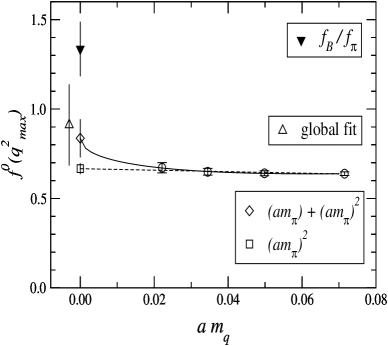
Figure 9:

Extrapolation of $f_{0}$ at the end point to the chiral limit by JLQCD [60]. The open triangle comes from a global fit to the form in Ref. [66].

Of course, one can always take the attitude that the SPR is irrelevant to phenomenology because there is no rate near the end point and, besides, it is $f_{+}$, not $f_{0}$, that determines the rate into $\pi\mu\nu$ or $\pi e\nu$. However, a credible demonstration of the SPR would be very helpful in convincing the non-lattice community that we have the form factor computation under control.

5 SPECTRA

Although I do not have space for a detailed review of recent spectral calculations for hadrons with one or more heavy quarks (Refs. [68, 69, 70, 71, 72, 73, 74, 75, 76, 77, 78, 79, 80]), I will make some remarks about a few features I find interesting and/or confusing:

(1) It seems clear that the computed quenched hyperfine splittings for heavy-light mesons are considerably smaller than the experimental values. For example, $M_{B_{s}^{*}}-M_{B_{s}}$ in the quenched approximation appears to be about half its physical value [68, 71, 72], although some older calculations e.g., Ref [81], found smaller ($\sim\!20\%$) discrepancies. For the $D_{s}$ system, the effect is also present at about the $20\%$ level in most [71, 82, 81] calculations (with one recent exception[70]). The sign and, very roughly, the magnitude of the observed discrepancy is expected from arguments about the effects of quark loops on the short distance potential. However, I know of no direct evidence from simulations that quenching is the culprit.

(2) There is a disagreement between Refs. [72] and [68] in the computed P-wave splittings for B mesons ($M_{B^{*}_{2}}-M_{B^{*}_{0}}$ or $M_{B^{*}_{0}}-M_{B}$, or the corresponding quantities for $B_{s}$). The disagreement is considerably larger than the systematic errors quoted by both groups and deserves further study. My guess is that the problem lies in excited state contamination: These mass differences are quite noisy, and it is seems very difficult to identify a “true plateau” in the effective mass plots.

(3) For NRQCD computations of splittings in charmonium, Stewart and Koniuk [75] confirm previous evidence [83] that the results are very sensitive to the order (in the velocity $v$) to which the Hamiltonian is corrected and how the tadpole improvement is done (plaquette or Landau link). Indeed, including the ${\cal O}(v^{6})$ terms, with the renormalization done at tadpole-improved tree level, moves the computed hyperfine splitting significantly further from experiment. I believe this is a “smoking gun” for renormalon shadow effects: At tadpole-improved tree level the presence of higher dimensional operators has no effect on the coefficients of lower dimensional operators — there is no subtraction of power law divergences. Just as for $f_{B}$, putting in the higher dimensional operators without the subtraction is then worse than leaving out those operators entirely. Unlike the $f_{B}$ case, however, the effect here appears to be numerically dramatic.

(4) In the $b\bar{b}$ system, NRQCD is clearly better behaved than in $c\bar{c}$, since the relativistic corrections are smaller. It is therefore possible to find convincing evidence for quenching effects [77, 73] if one is careful to keep other systematic effects (lattice spacing, order in $v$, type of tadpole improvement) fixed when comparing quenched and unquenched simulations. However, even for $b\bar{b}$, I believe it is important to reduce renormalon shadows by doing at least one-loop renormalization of the Hamiltonian before one can make reliable comparisons with experiment for most quantities.

(5) Following pioneering work by Klassen [84], there have been several recent simulations of charmonium on quenched “anisotropic relativistic” lattices [76, 77, 78]. The anisotropy $\xi$ is defined by $\xi\equiv a_{s}/a_{t}$, where $a_{s}$ and $a_{t}$ are the spatial and temporal lattice spacings, respectively. Choosing $\xi>1$ (typically $2\leq\xi\leq 5$) allows one to keep $a_{t}m_{Q}\ll 1$ and avoid large mass dependence in the improvement coefficients. Effectively, the heavy quark is relativistic. Although the improvement coefficients through ${\cal O}(a)$ can in principle be evaluated nonperturbatively, in practice the spatial and temporal clover coefficients are determined at tadpole-improved tree level, either by the Landau link or the plaquette.

Figure 10 shows the continuum extrapolation for the charmonium hyperfine splitting for various choices of anisotropy, tadpole factor, and scale determination. The good news is that the results from this method seem quite precise compared to previous relativistic calculations on isotropic lattices [86] and do not have the sensitive dependence on the tadpole factor seen [75, 83] in NRQCD. The bad news is that there appears to be some remaining dependence on the tadpole factor in the continuum limit (compare the open triangles and filled circles). The reason for the discrepancy is not yet clear. Additional data at larger $a_{s}$ with the plaquette tadpole may be useful in sorting out what is happening.

Figure 10:

Hyperfine splitting in charmonium vs. $a_{s}^{2}$ for relativistic anisotropic lattices. Data is from Refs. [84, 76, 77]; figure is taken from [77].

(6) The anisotropic relativistic approach has also been quite helpful in getting good signals for quarkonium hybrids [78]. As in glueball calculations [87], anisotropy gives more usable time slices before the signal is lost in noise. Another recent hybrid calculation [69] also employs anisotropic lattices, but in the NRQCD context.

(7) Kronfeld [79] has recently argued that a heavy quark on the lattice can be represented by a continuum HQET where the dependence on $am_{Q}$ is completely absorbed into the short-distance coefficients of the heavy quark operators. The operator matrix elements then only have mild lattice spacing dependence though the light degrees of freedom. This nice insight is then applied [80] to the heavy-light meson spectrum on the lattice in an attempt to compute the HQET parameters $\bar{\Lambda}$ and $\lambda_{1}$. ($\bar{\Lambda}$ is the meson binding energy in the static limit; $-\lambda_{1}/2m_{Q}$, the heavy quark kinetic energy.)

I have some concerns about Ref. [80]. One could find the continuum HQET by a two-step process: (a) for fixed $a$ in the lattice theory, take $m_{Q}$ large and arrive at a lattice HQET, and (b) order by order in perturbation theory, replace the lattice regularized HQET operators by their continuum counterparts. Although this not the procedure employed in [80], I believe the approaches should be equivalent. If I am right, then there are effective power law divergences and renormalon shadow effects in the coefficients of the continuum operators (resulting from step (b)). Therefore, a one-loop calculation may not be sufficiently accurate to extract $\bar{\Lambda}$ and $\lambda_{1}$. Indeed, parameterizing the discretization errors on $\bar{\Lambda}$ as $\bar{\Lambda}(a)=\bar{\Lambda}(0)(1-a{\cal M})$, the slope ${\cal M}$ has a value of $\approx\!0.65\;{\rm Ge\!V}$. Yet, if the lattice spacing dependence is coming only from the light degrees of freedom, which are at least tree-level improved through ${\cal O}(a)$, one expects ${\cal M}={\cal O}(\alpha_{s}\Lambda_{QCD})$, an order of magnitude smaller than what is found. This may be a renormalon shadow effect.

6 CONCLUDING REMARK

I have not made a unitarity triangle analysis with my world average lattice results. However, Fig. 11 shows the result of an analysis [88] that employs lattice values similar to those quoted here. Clearly, our knowledge of the triangle is getting quite precise. Over the last dozen years, the allowed region for the vertex has shrunk in area by almost a factor of 20, as is shown dramatically in Fig. 4 of Ref. [89]. We can be proud of the fact that lattice computations have played an important role in this accomplishment.

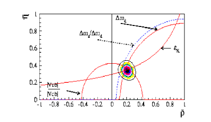
Figure 11:

Allowed region for the vertex of the unitary triangle (CKM parameters $\bar{\rho}$ and $\bar{\eta}$) from Ref. [88].

7 ACKNOWLEDGEMENTS

I thank A. Ali Khan G. Bali, D. Becirevic, R. Burkhalter, S. Gottlieb, R. Gupta, J. Hein, K.-I. Ishikawa, A. Kronfeld, L. Lellouch, R. Lewis, P. Mackenzie, T. Manke, G. Martinelli, C. Maynard, C. McNeile, M. Okamoto, T. Onogi, S. Ryan, H. Shanahan, S. Sint, R. Sommer and N. Yamada for discussion and private communication. This work was supported in part by the US Department of Energy under grant DE-FG02-91ER40628.

References

- [1] V. Lubicz, these proceedings.
- [2] G. Bali, hep-ph/0001312.
- [3] S. Hashimoto, Nucl. Phys. B (Proc. Suppl.) 83-84 (2000) 3.
- [4] T. Draper, Nucl. Phys. B (Proc. Suppl.) 73 (1999) 43.
- [5] A. El-Khadra et al., Phys. Rev. D58 (1998) 014506.
- [6] C. Allton et al., Phys. Lett. 405B (1997) 133.
- [7] S. Aoki et al., Phys. Rev. Lett. 80 (1998) 5711.
- [8] C. Bernard et al., Phys. Rev. Lett. 81 (1998) 4812.
- [9] A. Ali Khan et al., Phys. Lett. 427B (1998) 132.
- [10] K-I. Ishikawa et al., Phys. Rev. D61 (2000) 074501.
- [11] D. Becirevic et al., Phys. Rev. D60 (1999) 074501.
- [12] D. Becirevic et al., hep-lat/0002025.
- [13] K.C. Bowler, et al., hep-lat/0007020.
- [14] C. Maynard for UKQCD, these proceedings (hep-lat/0010016) and private communication.
- [15] R. Sommer, Nucl. Phys. B411 (1994) 839.
- [16] S. Datta for the MILC collaboration, these proceedings (hep-lat/0011029).
- [17] A. Ali Khan for CP-PACS, these proceedings; A. Ali Khan and H. Shanahan, private communications.
- [18] A. Ali Khan et al., hep-lat/0010009.
- [19] L. Lellouch and C.-J. Lin, private communication and hep-ph/0011086; contribution to Heavy Flavors 8, Southampton, England, 25-29 Jul 1999, hep-ph/9912322.
- [20] S. Collins et al., Phys. Rev. D60 (1999) 074504.
- [21] D. Becirevic for APE, these proceedings and private communication; Nucl. Phys. B (Proc. Suppl.) 83-84 (2000) 268.
- [22] Y. Iwasaki, Nucl. Phys. B258 (1985) 141.
- [23] R. Burkhalter for CP-PACS, these proceedings (hep-lat/0010078) and private communication.
- [24] E. Eichten, Nucl. Phys. B (Proc. Suppl.) 4 (1988) 170.
- [25] G.P. Lepage and B.A. Thacker, Nucl. Phys. B (Proc. Suppl.) 4 (1988) 199.
- [26] A. El-Khadra, A. Kronfeld and P. Mackenzie, Phys. Rev. D55 (1997) 3933.
- [27] G. Martinelli and C. Sachrajda, Nucl. Phys. B478 (1996) 660.
- [28] M. Beneke, Phys. Rept. 317 (1999) 1; G. Bodwin and Y.-Q. Chen, Phys. Rev. D60 (1999) 054008.
- [29] G. Martinelli and C. Sachrajda, Nucl. Phys. B559 (1999) 429.
- [30] G.P. Lepage and P. Mackenzie, Phys. Rev. D48 (1993) 2250.
- [31] M. Lüscher, et al., Nucl. Phys. B491 (1997) 323; ibid, 344.
- [32] K.-I. Ishikawa, T. Onogi, and N. Yamada, Nucl. Phys. B (Proc. Suppl.) 83-84 (2000) 301.
- [33] I thank K.-I. Ishikawa for providing me with their results for this subtraction coefficient.
- [34] C. Bernard and T. DeGrand, in preparation.
- [35] G. Parisi, in High Energy Physics — 1980, L. Durand and L.G. Pondrum, eds., (AIP, New York, 1981).
- [36] S. Collins et al., hep-lat/0007016.
- [37] O. Hernandez and B. Hill, Phys. Rev. D50 (1994) 495.
- [38] Y. Kuramashi, Phys. Rev. D58 (1998) 034507.
- [39] T. Bhattacharya et al., Nucl. Phys. B (Proc. Suppl.) 83-84 (2000) 851.
- [40] S. Sint and P. Weisz, Nucl. Phys. B502 (1997) 251.
- [41] T. Bhattacharya et al., hep-lat/0009038; talks by T. Bhattacharya and R. Gupta, these proceedings.
- [42] I thank S. Sint for pointing out an incorrect use of the equations of motion in an earlier version of NP-tad.
- [43] M. Kurth and R. Sommer, hep-lat/0007002; J. Heitger, M. Kurth and R. Sommer, in preparation and private communication.
- [44] C. Bernard et al., Nucl. Phys. B (Proc. Suppl.) 83-84 (2000) 289.
- [45] M. Albanese et al., Phys. Lett. 192B (1987) 163.
- [46] C. Bernard and T. DeGrand, Nucl. Phys. B (Proc. Suppl.) 83-84 (2000) 845.
- [47] M. Stephenson et al., hep-lat/9910023.
- [48] V. Gimenez and J. Reyes, Nucl. Phys. B545 (1999) 576 [raw data is taken from UKQCD (A.K. Ewing et al.), Phys. Rev. D54 (1996) 3526 and APE (V. Gimenez and G. Martinelli) Phys. Lett. 398B (1997) 135].
- [49] J. Christensen, T. Draper, and C. McNeile, Phys. Rev. D56 (1997) 6993.
- [50] N. Yamada for JLQCD, these proceedings (hep-lat/0010089) and private communication.
- [51] K.-I. Ishikawa et al., hep-lat/0004022 and these proceedings (hep-lat/0010056).
- [52] S. Hashimoto et al., Phys. Rev. D60 (1999) 094503; Phys. Rev. D62 (2000) 034504.
- [53] S. Sharpe, talk at ICHEP 98, Vancouver, Canada, July, 1998, hep-lat/9811006.
- [54] V. Gimenez and J. Reyes, these proceedings (hep-lat/0010048); hep-lat/0009007.
- [55] MILC collaboration, work in progress.
- [56] M. Booth, Phys. Rev. D51 (1995) 2338; S. Sharpe and Y. Zhang, Phys. Rev. D53 (1996) 5125.
- [57] R. Gupta et al., Phys. Rev. D55 (1997) 4036.
- [58] D. Becirevic et al., hep-ph/0006135.
- [59] K.C. Bowler et al., Phys. Lett. 486B (2000) 111; C. Maynard for UKQCD, Nucl. Phys. B (Proc. Suppl.) 83-84 (2000) 322.
- [60] T. Onogi for JLQCD, these proceedings (hep-lat/0011008) and private communication.
- [61] S. Ryan, A. Kronfeld and P. Mackenzie, private communications; S. Ryan et al., Nucl. Phys. B (Proc. Suppl.) 83-84 (2000) 328.
- [62] J. Shigemitsu et al., these proceedings (hep-lat/0010029).
- [63] D. Becirevic and A. Kaidalov, Phys. Lett. 478B (2000) 417.
- [64] K.C. Bowler et al., Phys. Rev. D51 (1995) 4905.
- [65] G. Burdman and J.F. Donoghue, Phys. Lett. 280B (1992) 287; M.B. Wise, Phys. Rev. D45 (1995) 2188; N. Kitazawa and T. Kurimoto Phys. Lett. 323B (1994) 65.
- [66] G. Burdman et al., Phys. Rev. D49 (1994) 2331.
- [67] H. Matsufuru et al., Nucl. Phys. B (Proc. Suppl.) 63 (1998) 368; S. Aoki, ibid, 380.
- [68] A. Ali Khan et al., Phys. Rev. D62 (2000) 054505.
- [69] I.T. Drummond et al., Phys. Lett. 478B (2000) 151.
- [70] R.M. Woloshyn, Phys. Lett. 476B (2000) 309.
- [71] J. Hein et al., Phys. Rev. D62 (2000) 074503 and private communication.
- [72] R. Lewis and R.M. Woloshyn, hep-lat/0003011; these proceedings (hep-lat/0010001) and private communication.
- [73] C. Davies, these proceedings (L. Marcantonio et al., hep-lat/0011053).
- [74] T. Manke et al., hep-lat/0005022.
- [75] C. Stewart and R. Koniuk, hep-lat/0005024 and these proceedings (hep-lat/0010015).
- [76] P. Chen, hep-lat/0006019.
- [77] M. Okamoto for CP-PACS, these proceedings (hep-lat/0011005) and private communication.
- [78] P. Chen, X. Liao and T. Manke, these proceedings (hep-lat/0010069); T. Manke, private communication.
- [79] A. Kronfeld, Phys. Rev. D62 (2000) 014505 and private communication.
- [80] A. Kronfeld and J. Simone, Phys. Lett. 490B (2000) 228.
- [81] R. Lewis and R.M. Woloshyn, Phys. Rev. D58 (1998) 074506.
- [82] P. Mackenzie, Nucl. Phys. B (Proc. Suppl.) 63 (1998) 305; P. Boyle (UKQCD), ibid, 314.
- [83] H.D. Trottier, Phys. Rev. D55 (1997) 6844; N.H. Shakespeare and H.D. Trottier, Phys. Rev. D58 (1998) 034502.
- [84] T. Klassen, Nucl. Phys. B533 (1998) 557; Nucl. Phys. B (Proc. Suppl.) 73 (1999) 918; and unpublished.
- [85] I thank A. Kronfeld for this remark.
- [86] Reference [76] compares, for example, to unpublished work from the Fermilab group.
- [87] C. Morningstar and M. Peardon, Phys. Rev. D56 (1997) 4043.
- [88] M. Ciuchini et al., paper submitted to ICHEP 2000, Osaka, 27 July – 2 August, 2000.
- [89] F. Caravaglios et al., hep-ph/0002171.