Finite size scaling analysis of compact QED

Abstract

We describe results of a high-statistics finite size scaling analysis of 4d compact U(1) lattice gauge theory with Wilson action at the phase transition point. Using a multicanonical hybrid Monte Carlo algorithm we generate data samples with more than 150 tunneling events between the metastable states of the system, on lattice sizes up to $18^{4}$. We performed a first analysis within the Borgs-Kotecky finite size scaling scheme. As a result, we report evidence for a first-order phase transition with a plaquette energy gap, $G=0.02667(20)$, at a transition coupling, $\beta_{T}=1.011128(11)$.

1 INTRODUCTION

The determination of the order of phase transitions is of high importance for lattice field theories. For it requires higher than first-order phase transitions to make contact between lattice and continuum physics.

In compact quantum electrodynamics (QED) with Wilson action the order of the transition between the confined and Coulomb phases has been under debate for many years[1]. On the scale of accessible lattice sizes the correlation length is large, but the system exhibits a definite two-peak structure.

In a recent high statistics investigation[1] the latent heat appeared to decrease with the lattice size $L$, with a critical exponent $\nu$ being neither 0.25 (first order) nor $0.5$ (trivially second order), with significant subasymptotic contributions at the studied values of $L\leq 12$. These findings allow for two scenarios:

1. The observed double peak structure is a finite size effect and vanishes in the thermodynamic limit. The signature of a second-order phase transition would eventually emerge at some $L_{0}\gg 12$.

2. The phase transition is weakly first-order, i. e., the correlation length $\xi$ remains finite, yet large in terms of lattice extensions accessible today; this would fake, on small lattices, the signature of a second-order transition, since the true value of the latent heat would be revealed only in the regime $L>\xi$ .

For a class of spin models with strong first-order phase transitions finite size scaling theory has become amenable to quantitive studies through the work of Borgs and Kotecky[2, 3, 4]. There the finite volume partition function at temperature $\beta$ in finite volumes with periodic boundary conditions (neglecting interfacial contributions) has the remarkably simple form

$$Z=[e^{-Vf_{1}(\beta)}+e^{-Vf_{2}(\beta)+\ln(X)}]\;.$$ (1)

The functions $f_{1}(\beta)$ and $f_{2}(\beta)$ denote bulk free energy densities in the two coexisting phases 1 and 2. $X$ denotes the asymmetry parameter which is nothing but the relative phase weight in the probability distribution $P(E)$.

In Ref.[5] the Borgs-Kotecky ansatz has been extended in a heuristic manner to the 3d 3-state Potts model undergoing a weakly first-order phase transition; in this instance detailed consistency checks have been carried out in order to verify the viability of the Borgs-Kotecky approach. Motivated by this success we shall apply in the following this ansatz to compact QED lattice gauge theory.

2 SIMULATION DETAILS

We consider 4d pure U(1) gauge theory with standard Wilson action

$$S=-\beta\sum_{n,\nu>\mu}\cos(\theta_{\mu\nu}(n)),$$ (2)

where $\beta$ denotes the Wilson coupling and $\theta_{\mu\nu}(n)$ the plaquette angle. We use a cubic lattice of volume $V=L^{4}$ with periodic boundary conditions.

We have implemented three different algorithms for generating the U(1) gauge field configurations: (a) a local Metropolis (MRS), updating each link separately, (b) a global hybrid Monte Carlo algorithm (HMC) and (c) a combination of the multicanonical and the hybrid Monte Carlo algorithm (MHMC). For details we refer to Refs. [6, 7]. Each update of the complete lattice is followed by 3 reflection steps[8] to reduce correlation of successive configurations. The number of generated configurations at each lattice size $L$ is $\geq 2.5\times 10^{6}$. We additionally measure the number of tunneling events (flips) as control parameter for the mobility of the algorithms.

Our simulation parameters and the statistics achieved are listed in Table 1. As the runs differing by algorithm, HMC parameters or by weight function are independent we do not recombine them into one multihistogram. Rather we treat them separately.

Table 1: Number of configurations generated on different lattice sizes. In case of HMC generated data the time step $\Delta t$ and trajectory length $N_{md}$ is specified. The MHMC runs with equal parameter settings differ by the choice of weight parameters.

L	$\beta$	algorithm	$\Delta t$	$N_{md}$	iterations	flips
6	1.001600	HMC	.120	10	2500000	3581
8	1.007370	HMC	.093	2	1250000	276
	1.007370	HMC	.093	4	1250000	557
	1.007370	HMC	.093	6	1250000	707
	1.007370	HMC	.093	8	1250000	856
	1.007370	HMC	.093	9	1250000	913
	1.007370	HMC	.093	10	1250000	932
	1.007370	HMC	.093	11	1250000	935
	1.007370	HMC	.093	12	1250000	921
	1.007370	HMC	.093	13	1250000	935
	1.007370	HMC	.093	14	1250000	859
	1.007370	HMC	.093	16	1250000	862
	1.007370	HMC	.093	13	1440000	1265
10	1.009300	HMC	.071	9	1000000	294
	1.009300	HMC	.071	11	1000000	350
	1.009300	HMC	.071	15	1000000	351
	1.009300	HMC	.071	17	1000000	344
	1.009300	HMC	.071	19	1000000	340
12	1.010143	MRS			3617000	571
		MHMC	.060	20	1303500	407
14	1.010598	MRS			3900000	215
	1.010568	MHMC	.050	24	825200	186
16	1.010753	MRS			3460000	45
	1.010753	MHMC	.045	26	595000	73
	1.010753	MHMC	.045	26	626000	83
	1.010753	MHMC	.045	20	1044000	189
18	1.010900	MHMC	.042	28	632000	23
	1.010900	MHMC	.042	28	905700	68
	1.010900	MHMC	.042	28	980000	61
	1.010900	MHMC	.042	28	380000	15

3 MEASUREMENTS

Based on the plaquette operator

$$E=\frac{1}{6V}\sum_{n,\nu>\mu}\cos(\theta_{\mu\nu}(n)).$$ (3)

we consider the following cumulants:

$$C_{v}(\beta,L) = 6\beta^{2}\,V\left(\left<E^{2}\right>-\left<E\right>^{2}\right),$$ (4)

$$U_{2}(\beta,L) = 1-\frac{\left<E^{2}\right>}{\left<E\right>^{2}},$$ (5)

$$U_{4}(\beta,L) = \frac{1}{3}\left(1-\frac{\left<E^{4}\right>}{\left<E^{2}\right>^{2}}\right).$$ (6)

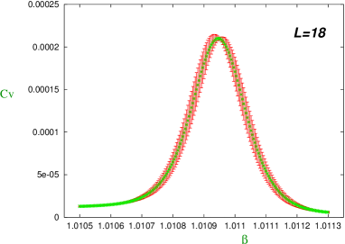
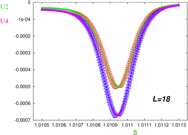
Figure 1: The measured cumulants of our data at $L=18$ taken from the third run in table 1 reweighted to different couplings $\beta$ in order to determine their extrema.

The locations $(\beta_{c},C_{v,max})$ and $(\beta_{c},U_{i,min})$ of their extrema are determined by reweighting the measured probability distribution $P(E)$ to different couplings $\beta$ (see Fig 1). To calculate the estimates of our cumulants at each lattice size $L$ we proceed in two steps: i) determine the error of each individual run performing a jackknife error analysis by subdivision of the run into ten blocks; ii) calculate the final result by $\chi^{2}$-fitting these individual run results to a constant. The $L$-dependence of the latter is quoted in Table 2 and 3.

Table 2: Locations of the specific heat maxima as a function of lattice size.

L	$\beta_{c}$	$C_{v,max}/6V\times 10^{-4}$
6	1.001794(64)	9.7728(497)
8	1.007413(14)	5.5428(105)
10	1.009383(16)	3.8535(130)
12	1.010229(14)	2.9813(118)
14	1.010626(11)	2.5470(139)
16	1.010840(9)	2.2620(161)
18	1.010943(8)	2.1154(152)

Table 3: Locations of the $U_{i}$ minima.

L	$\beta_{U_{2}}$	$U_{2,min}\times 10^{-3}$
6	1.001383(63)	-2.5815(136)
8	1.007306(14)	-1.3954(27)
10	1.009344(16)	-0.9481(33)
12	1.010212(14)	-0.7241(29)
14	1.010617(11)	-0.6142(35)
16	1.010836(9)	-0.5428(40)
18	1.010940(8)	-0.5063(37)

L	$\beta_{U_{4}}$	$U_{4,min}\times 10^{-3}$
6	1.001174(63)	-3.4489(182)
8	1.007241(14)	-1.8627(36)
10	1.009319(16)	-1.2651(44)
12	1.010200(14)	-0.9661(39)
14	1.010610(11)	-0.8194(46)
16	1.010832(9)	-0.7241(53)
18	1.010938(8)	-0.6753(50)

4 FINITE SIZE SCALING ANALYSIS

Under the assumption that the phase transition is discontinuous, the Borgs-Kotecky representation of the partition function suggests, that both, the maxima of the specific heat $C_{v,max}$ and the pseudocritical $\beta$-values can be expanded in terms of th in the inverse volume,

$$\frac{C_{v,max}(V)}{6V}=\frac{1}{4}G^{2}+\sum_{k=1}^{\infty}A_{k}V^{-k}$$ (7)

and

$$\beta_{c}(V)=\beta_{T}+\sum_{k=1}^{\infty}B_{k}V^{-k}.$$ (8)

The quantity $G$ stands for the infinite volume gap in the plaquette energy and $\beta_{T}$ denotes the infinite volume transition point of the system. We fit our data for $C_{v,max}$ and $\beta_{c}$ (given in Table 2) to the parameterizations, Eq. 7 and 8.

In order to expose systematic effects in the fit parameter $G$, we vary the fit range with various ranges $L_{min}\leq L\leq 18$ as well as the truncation parameter $k_{max}$. The results in $G$ are given in Table 4. It is possible to apply the parameterization of Eq. 7 down to $L_{min}=6$ if one increases $k_{max}$ such that one degree of freedom remains. It is nice to see that results with $\chi^{2}_{dof}<1$ are completely consistent.

To illustrate the fit stability we additionally included the lowest expansion coefficients $A_{1}$ into Table 4. Note that here again $\chi^{2}_{dof}<1$ results exhibit complete stability.

The observed stability pattern supports the validity of the $V^{-1}$-expansion. This corroborates the previous analysis [1] on lattices up to $L=12$.

Table 4: Fit values of the infinite volume gap $G$ according to Eq. 7. Fit results in bold face correspond to good quality fits ($\chi^{2}_{dof}<1$).

$Range$	$k_{max}$	$\chi^{2}_{dof}$	$G$	$A_{1}$
14-18	1	1.03	0.02731(17)	2.62(12)
12-18	1	6.65	0.02779(27)	2.20(11)
	2	0.50	0.02698(18)	3.22(20)
10-18	1	25.9	0.02837(37)	1.88(9)
	2	7.76	0.02746(22)	2.61(15)
	3	0.72	0.02686(26)	3.47(34)
8-18	1	202	0.02965(73)	1.40(8)
	2	7.93	0.02788(24)	2.26(9)
	3	2.21	0.02737(22)	2.72(16)
	4	0.80	0.02682(29)	3.57(41)
6-18	1	681	0.03066(12)	1.22(12)
	2	113	0.02913(60)	1.64(10)
	3	5.54	0.02777(21)	2.36(9)
	4	2.17	0.02735(22)	2.75(17)
	5	0.83	0.02681(31)	3.60(44)

Table 5: Infinite volume transition coupling $\beta_{T}$ obtained by fitting Eq. 8. Fit results in bold face correspond to good quality fits.

$Range$	$k_{max}$	$\chi^{2}_{dof}$	$\beta_{T}$	$B_{1}$
14-18	1	0.47	1.0111220(95)	-18.81(56)
12-18	1	0.36	1.0111169(56)	-18.46(24)
	2	0.59	1.0111238(166)	-19.14(151)
10-18	1	3.62	1.0110978(124)	-17.39(33)
	2	0.83	1.0111288(123)	-19.65(44)
	3	0.67	1.0111207(196)	-18.71(210)
8-18	1	45.5	1.0110437(370)	-15.13(43)
	2	0.44	1.0111212(80)	-19.08(20)
	3	0.36	1.0111299(82)	-19.79(57)
6-18	1	224	1.0109952(785)	-13.99(78)
	2	17.8	1.0110760(244)	-16.72(42)
	3	0.29	1.0111257(45)	-19.44(18)
	4	0.36	1.0111264(85)	-19.81(62)

As our final result for the infinite volume gap we obtain

$$G=0.02698(18)(17).$$ (9)

We proceed similarly in fitting the pseudocritical coupling $\beta_{T}$, Eq. 8, with results given in Table 5. From our analysis of $C_{v}$ we obtain the critical Wilson coupling $\beta_{T}=1.011122(10)(8)$.

As a further consistency check we analyze in addition the cumulants $U_{2}$ and $U_{4}$ with parameterizations analogous to Eq. 8.

Table 6: Results for the transition coupling $\beta_{T}$ obtained by analysis of three different cumulants.

cumulant	$\beta_{T}$
$C_{v}$	1.011122(10)(8)
$U_{2}$	1.011129(14)(8)
$U_{4}$	1.011132(6)(10)

All three estimates (see Table 6) are in complete agreement within their statistical errors. We view this as a confirmation of the validity of Borgs-Kotecky FSS as applied to compact QED. As final we quote the average of the values given in Table 6.

$$\beta_{T}=1.011128(11).$$ (10)

It remains to be seen whether our data exclude the possibility of a continuous singular behaviour with a vanishing infinite volume gap. Under this alternative assumption one expects the asymptotic scaling laws

$$C_{v,max}(L)=C_{1}L^{\frac{2}{\nu}-8}$$ (11)

and

$$\beta_{c}(L)=\beta_{T}+aL^{-\frac{1}{\nu}}.$$ (12)

Here $\nu$ denotes the critical exponent of the correlation length as hyperscaling is assumed.

Our data clearly disfavour the validity of Eq. 11 for any range of $L$-values. For Eq. 12 however we find the fit parameters as quoted in Table 7.

Table 7: Fit results obtained from second-order scaling in Eq. 12.

$L_{min}$	$\chi^{2}_{dof}$	$\beta_{T}$	$\nu^{-1}$
6	5.12	1.011247(26)	3.20(5)
8	2.17	1.011204(22)	3.34(7)
10	0.69	1.011158(20)	3.61(11)
12	0.64	1.011127(32)	3.90(29)

Note that fit stability cannot be reached under variation of the fit intervals $L_{min}\leq L\leq 18$, neither in $\beta_{T}$ nor in $\nu$. However it cannot be excluded, that corrections to scaling could lead to stable fits also in this scenario.

5 DIRECT APPROACH TO LATENT HEAT

Having determined $\beta_{T}$ very accurately within Borgs-Kotecky FSS theory we are now in the position to make a ’direct’ measurement of the latent heat based on our determination of $\beta_{T}$ . Using the conventional canonical algorithm we generate $O(10^{5})$ configurations of each metastable phase simulating systems of size $L=6,8,\ldots,24,28,32$ at $\beta_{T}$ as given in Eq. 10 and locate the positions of the energy peaks in the confined and Coulomb phase denoted by $E_{1}$ and $E_{2}$. As shown in Fig. 2 we fit our data for each phase separately to a Gaussian of the form $a\exp(-b(E-E_{i})^{2})$. Note that one cannot extract the relative phase weight from Fig. 2, because it depicts the probability distributions $P_{i}(E)$ of two independent runs $i=1,2$ without any flip.

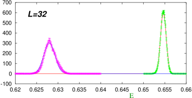
Figure 2: Separate fit of each measured phase peak of the $L=32$ system at $\beta_{T}$ to a Gaussian.

Fig. 3 shows these peak positions $E_{i}(L)$ as a function of lattice size $L$. It is a prediction of the Borgs-Kotecky scheme that they deviate from their infinite volume value $E_{i}(\infty)$ by exponentially small terms only. Accordingly we fit both branches to

$$E_{i}(L)=E_{i}(\infty)+a_{i}e^{-b_{i}L},$$ (13)

achieving high fit quality with $\chi^{2}_{dof,1}=0.40$ and $\chi^{2}_{dof,2}=0.58$. Fig. 4 illustrates the data and the fitted branches on an expanded energy scale. Due to the wider distributed peak of the confinement phase the errors of the lower branch $E_{1}(L)$ are larger than in case of $E_{2}(L)$.

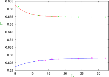
Figure 3: Peak positions $E_{i}$ as a function of lattice size $L$.

Figure 4: Data fitted to Eq. 13 on an expanded energy scale.

With the fit results $E_{i}(\infty)$ we are in the position to present a high precision measurement of the infinite volume energy gap,

$$\hat{G}=E_{2}(\infty)-E_{1}(\infty)=0.02667(20).$$ (14)

The estimate obtained from first-order scaling of the specific heat as given in Eq. 9 is in agreement with this result. This presents a further support to the applicability of Borgs-Kotecky FSS to U(1) gauge theory.

6 SUMMARY AND CONCLUSIONS

All cumulants investigated in our high statistics analysis at $L=6,8,10,12,14,16,18$ are in accord with Borgs Kotecky first-order FSS. Our data does not favour second-order FSS as indicated by large $\chi^{2}$ and lacking convergence of the critical exponent $\nu$. Within the framework of Borgs-Kotecky we determined the infinite volume transition coupling with a relative error of the order of $10^{-5}$. A direct investigation of the latent heat at $\beta_{T}$ for system sizes up to $L=32$ yields a non-vanishing infinite volume energy gap $\hat{G}$ with an error of 1%. The systematic error of the energy gap due to the error of $\beta_{T}$ is of the same order as its statistical error. The gap $G=0.02698(18)(17)$ extracted from first-order FSS of the specific heat is in agreement with the direct measurement of $\hat{G}$.

The material presented here is a progress report. In a forthcoming paper we shall elaborate further on systematic effects.

References

- [1] B. Klaus and C. Roiesnel: Phys. Rev. D58 (1997) 114509.
- [2] C. Borgs and R. Kotecky: J. Stat. Phys. 61 (1990) 79.
- [3] C. Borgs and R. Kotecky: Phys. Rev. Lett. 68 (1992) 1734.
- [4] C. Borgs, R. Kotecky and S. Miracle–Sole: J. Stat. Phys. 62 (1991) 529.
- [5] W. Janke and R. Villanova: Nucl.Phys. B489 (1997) 679-696.
- [6] G. Arnold, Th. Lippert and K. Schilling: Phys.Rev. D59 (1999) 054509.
- [7] G. Arnold, Th. Lippert and K. Schilling: Nucl.Phys.Proc.Suppl. 83 (2000) 768-770.
- [8] B. Bunk: proposal for U(1) update, unpublished, private communication.