Computer Simulations of 3d Lorentzian Quantum Gravity

Abstract

We investigate the phase diagram of non-perturbative three-dimensional Lorentzian quantum gravity with the help of Monte Carlo simulations. The system has a first-order phase transition at a critical value $k_{0}^{c}$ of the bare inverse gravitational coupling constant $k_{0}$. For $k_{0}>k_{0}^{c}$ the system reduces to a product of uncorrelated Euclidean 2d gravity models and has no intrinsic interest as a model of 3d gravity. For $k_{0}<k_{0}^{c}$, extended three-dimensional geometries dominate the functional integral despite the fact that we perform a sum over geometries and no particular background is distinguished at the outset. Furthermore, all systems with $k_{0}<k_{0}^{c}$ have the same continuum limit. A different choice of $k_{0}$ corresponds merely to a redefinition of the overall length scale.

1 INTRODUCTION

We still need to find the theory of quantum gravity. In [1, 2] we have proposed a dynamically triangulated model of two, three and four dimensional quantum gravity with the following properties:
(a) Lorentzian space-time geometries (histories) are obtained by causally gluing sets of Lorentzian building blocks, i.e. $d$-dimensional simplices with simple length assignments;
(b) all histories have a preferred discrete notion of proper time $t$; $t$ counts the number of evolution steps of a transfer matrix between adjacent spatial slices, the latter given by $(d\!-\!1)$-dimensional triangulations of equilateral Euclidean simplices;
(c) each Lorentzian discrete geometry can be “Wick-rotated” to a Euclidean one, defined on the same (topological) triangulation;
(d) at the level of the discretized action, the “Wick rotation” is achieved by an analytic continuation in the dimensionless ratio $\alpha\!=\!-l^{2}_{\rm t}/l^{2}_{\rm s}$ of the squared time- and space-like link length; for $\alpha\!=\!-1$ one obtains the usual Euclidean action of dynamically triangulated gravity;
(e) the extreme phases of degenerate geometries found in the Euclidean models cannot be realized in the Lorentzian case.

A metric space-time is constructed by “filling in” for all $t$ the $d$-dimensional sandwich between the pair of spatial slices at integer times $t$ and $t\!+\!1$. We only consider regular gluings which lead to simplicial manifolds. In the case of three-dimensional quantum gravity the basic building blocks are three types of Lorentzian tetrahedra, (1): (3,1)-tetrahedra (three vertices contained in slice $t$ and one vertex in slice $t+1$): they have three space- and three time-like edges; their number in the sandwich $[t,t\!+\!1]$ will be denoted by $N_{31}(t)$; (2): (1,3)-tetrahedra: the same as above, but upside-down; the tip of the tetrahedron is at $t$ and its base lies in the slice $t+1$; notation $N_{13}(t)$; (3): (2,2)-tetrahedra: one edge (and therefore two vertices) at each $t$ and $t+1$; they have two space- and four time-like edges; notation $N_{22}(t)$.

Each of these triangulated space-times carries a causal structure defined by the piecewise flat Lorentzian metric. Each time-like link is given a future-orientation in the positive $t$-direction, so that two lattice vertices connected by a sequence of positively oriented links are causally related.

As mentioned in (d) above, after rotating to Euclidean signature and choosing $\alpha=\!-\!1$, the Einstein action becomes identical to the action

$$S_{\rm E}(N_{0},N_{3},T)=-k_{0}N_{0}+k_{3}N_{3}$$ (1)

used in Euclidean dynamical triangulations [3], where $N_{0}$ and $N_{3}$ denote the total numbers of vertices and tetrahedra in the triangulation. The dimensionless couplings $k_{0}$ and $k_{3}$ have been introduced to conform with the conventions used in 3d Euclidean simplicial quantum gravity. Here $k_{0}$ is proportional to the bare inverse gravitational coupling constant, while $k_{3}$ is a linear combination of the bare cosmological and inverse gravitational constants. In a slight abuse of language, we will still refer to $k_{3}$ as the (bare) cosmological constant. We fix the space-time topology to $S^{1}\times S^{2}$, where the periodic identification in the $t$-direction has been chosen entirely for practical convenience. The total length of the space-time in the compactified $S^{1}$-direction (i.e. the number of proper-time steps) is denoted by $T$. The partition function is thus

$$Z(k_{0},k_{3},T)=\sum_{{\cal T}_{T}(S^{1}\times S^{2})}\mbox{e}^{-S_{\rm E}(N_{0},N_{3},T)},$$ (2)

where the sum is taken over the class ${\cal T}_{T}(S^{1}\times S^{2})$ of triangulations of $S^{1}\times S^{2}$ specified earlier, for fixed $T$. While (2) is similar in structure to the standard partition function of dynamically triangulated Euclidean gravity, one should bear in mind that the set of triangulations contributing in (2) is quite different.

2 THE MONTE CARLO SIMULATION

We explore the phase diagram of the theory defined by the state sum (2) using Monte Carlo simulations. A 3d triangulation in the sum (2) consists of $t$ successive 2d triangulations. These spatial slices are glued together by filling the space-time gaps between them with the three types of building blocks described in the introduction.

A local updating algorithm consisting of five basic moves changes one such triangulation into another one, while preserving the constant-time slice structure. A successive application of these moves will take us around in the class of triangulation with fixed $T$. The moves are (see [4] for more details):
(1): consider two neighbouring triangles in the spatial $t$-plane such that the two associated pairs of tetrahedra above and below the $t$-plane each share one triangle. We can perform a standard “flip” move of the link common to the two triangles in the $t$-plane and make a corresponding reassignment of tetrahedra. (2&3): Consider a triangle in the spatial $t$-plane and insert a vertex at its centre. In this way the two neighbouring tetrahedra sharing the triangle are replaced by six tetrahedra, three above and three below. There is an obvious inverse move. (4&5): The fourth move is the standard Alexander move performed on a (2,2)-tetrahedron and a (3,1)-tetrahedron sharing a triangle, replacing it by two (2,2)- and one (3,1)-tetrahedra, and the fifth move is its inverse. Obviously the (3,1)-tetrahedron could have been replaced by a (1,3)-tetrahedron in (4&5).

The strategy for the simulations is the usual one from dynamical triangulations: fine-tune the cosmological constant to its critical value $k^{c}_{3}(k_{0})$ (which depends on the bare inverse gravitational coupling constant $k_{0}$) and keep the fluctuations of space-time volume bounded within a certain range. Then measure expectation values of suitable observables for these quantum universes.

3 RESULTS

In order to explore the phase diagram of our regularized model we have to identify an order parameter, and explore how it changes with the coupling constant, in this case $k_{0}$. We have found that the ratio $\tau$ between the total number $N_{22}$ of (2,2)-tetrahedra and the total space-time volume

$$N_{3}\equiv N_{tot}=N_{22}+N_{31}+N_{13}$$

serves as an efficient order parameter. In Fig. 1 we show $\tau$ as a function of $k_{0}$. One observes a rapid drop to zero of $\tau(k_{0})$ around $k_{0}\approx 6.64$. Increasing $N_{3}$, the drop becomes a jump, typical for a first-order phase transition. A detailed study of the neighbourhood of $k_{0}\!=\!6.64$ reveals a hysteresis as one performs a cycle, moving above and below the critical value $k_{0}^{c}$, again as expected from a first-order transition.

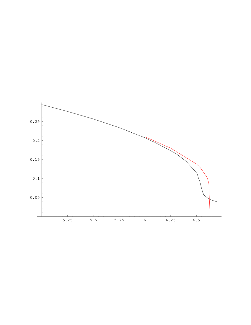
Figure 1: The order parameter $\tau=N_{22}/N_{tot}$ for configurations with $T\!=\!64$, and $N_{3}\!=\!16,000$ (black curve) and 64,000 (red curve), plotted as a function of $k_{0}$.

The phase above $k_{0}^{c}$ is of no interest for continuum 3d quantum gravity since one can show that it is equivalent to an uncorrelated product of 2d Euclidean gravity models [4].

We now turn to the interesting phase of $k_{0}<k_{0}^{c}$. Remarkably, we observe here the emergence of well-defined three-dimensional configurations. In Fig. 2 we present a snapshot of a configuration of 16,000 tetrahedra for $k_{0}\!=\!5.0$ and of total proper-time extent $T\!=\!32$. It shows the 2d spatial volume as a function of the time $t$. Following the computer-time history of this extended object, it is clear that although it does indeed fluctuate, the fluctuations take place around a three-dimensional object of a well-defined linear extension. The emergence of a ground state of extended geometry is a very non-trivial property of the model, since we never put in any preferred background geometry by hand. No structures of this kind have ever been observed in dynamically triangulated models of Euclidean quantum gravity. It underscores the fact that the Lorentzian models are genuinely different and affirms our conjecture that in $d\geq 3$ they are less pathological than their Euclidean counterparts.

Figure 2: Snapshot of the distribution of 2d volumes $N_{31}(t)$ of spatial slices at times $t\in[0,T]$, with $T\!=\!32$ and $k_{0}\!=\!5.0$ ($k_{0}^{c}\!=\!6.64$).

Let us denote the typical time-extent of our extended “universe” by $T_{u}$. We will always choose the total proper time $T$ sufficiently large, such that $T_{u}<T$ for the range of $N_{3}$ under consideration. Since both the shape of the universe and its location along the $t$-direction fluctuate, we have found it convenient to measure the correlation function

$$C(\Delta)=\frac{1}{{T}^{2}}\sum_{t=1}^{T}\langle N_{2s}(t)N_{2s}(t+\Delta)\rangle,$$ (3)

where $N_{2s}(t)\!=\!N_{13}(t)+N_{31}(t)+N_{22}(t)$, as a function of the displacement $\Delta$ to determine the scaling of $T_{u}$ with the space-time volume $N_{3}$. This correlator has the advantage of being translation-invariant in $t$ and allows for a precise measurement by averaging over many independent configurations. From the typical shape of the space-time configurations we expect $C(\Delta)$ to be of the order of the spatial cut-off if $\Delta\gg 2T_{b}$. Fig. 3 illustrates the result of our measurements of $C(\Delta)$, with the dots representing the measured values.

Figure 3: The correlator $C(\Delta)$ with $T\!=\!64$ and $N_{3}\!=\!32,000$. Dots are the measured values (error bars less than dots), and the curve is fitted from the sphere solution described in the text.

The theoretical curve to which we are fitting corresponds to a sphere $S^{3}$ with the radius as a free parameter. (By $S^{3}$ we mean the 3d geometry of constant positive curvature which is a classical solution of Euclidean gravity with a positive cosmological constant.) In order to “adapt” the $S^{3}$-solution to the topology $S^{1}\times S^{2}$, we assume that the standard $S^{3}$-solution is valid until the radius $r$ of the $S^{2}$-slice reaches the spatial cut-off scale. Beyond this point, the value of $r$ is frozen to the cut-off value, which we also take as a free parameter. For this “spherical” geometry we then perform the integral (the sum) in (3), without the average $\langle\cdot\rangle$. As is evident from Fig. 3, the volume distribution associated with this fixed geometry gives a rather good fit to our data. This provides some evidence that we can ignore the quantum average implied by $\langle\cdot\rangle$, and that our universes behave semi-classically, at least as far as their macroscopic geometric properties are concerned. We should mention that our “$S^{3}$-solution” is not singled out uniquely, since the choice of a Gaussian shape in the $t$-direction gives a fit of comparable quality.

For various space-time volumes $N_{3}$ (typically 8, 16, 32 and 64k) we have determined the radius $R_{S^{3}}$ of $S^{3}$ from the fits to the measured $C(\Delta)$. From this, we have finally found $\alpha=0.34\pm 0.02$ as the best exponent in the scaling relation

$$R_{S^{3}}(N_{3})=N_{3}^{\alpha}.$$ (4)

The same value is obtained using other ways to extract $T_{u}$, lending additional support to the genuinely three-dimensional nature of our universes.

Another important result concerns the relation between the geometries of different $k_{0}$, in the phase where $k_{0}<k_{0}^{c}$. In the numerical simulations we have observed the following: (i) the distributions as functions of $t$ can be made to coincide for different $k_{0}$ by rescaling the time, $t\to f_{ti}(k_{0})t$ or $a_{t}\to f_{ti}(k_{0})a_{t}$, where $a_{t}$ is the link length in time direction. (ii) The distributions measured in the spatial slices from inside the universe can be made to coincide for different $k_{0}$ by rescaling the spatial link distance $a_{s}\to f_{sp}(k_{0})a_{s}$, where $a_{s}$ is the length of the spatial links. This is illustrated in Fig. 4 for the distributions of 2d volumes $V(l)$ of spatial spherical shells of (link) radius $l$, measured for various values of $k_{0}$.

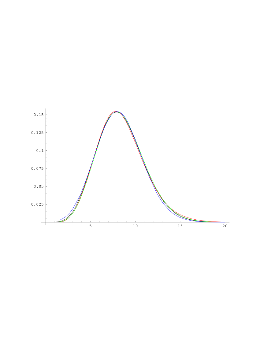
Figure 4: The 2d volume $V(l)$ of spatial spherical shells, measured only on slices inside the spherical universe, for various $k_{0}$ and rescaled, using the seemingly unrelated scaling obtained by applying the same philosophy to the correlator $C(\Delta)$.

(iii) Within the numerical accuracy we find that $f_{ti}(k_{0})=f_{sp}(k_{0})$.

We conclude that apart from the overall length scale of the universe, set by the bare inverse gravitational coupling $k_{0}$, the physics is the same for all values $k_{0}$ below $k_{0}^{c}$.

References

- [1] J. Ambjørn and R. Loll, Nucl. Phys. B536 (1998) 407.
- [2] J. Ambjørn, J. Jurkiewicz and R. Loll, Phys. Rev. Lett. 85 (2000) 924.
- [3] J. Ambjørn and J. Jurkiewicz, Phys. Lett. B278 (1992) 42.
- [4] J. Ambjørn, J. Jurkiewicz and R. Loll, Non-perturbative 3d Lorentzian quantum gravity, to appear.