MAXIMUM ENTROPY ANALYSIS
OF THE SPECTRAL FUNCTIONS IN LATTICE QCD
M. Asakawa⁽¹⁾, T. Hatsuda⁽²⁾ and Y. Nakahara⁽¹⁾

⁽¹⁾ Department of Physics, Nagoya University, Nagoya 464-8602, Japan

⁽²⁾ Department of Physics, University of Tokyo, Tokyo 113-0033, Japan

Abstract

First principle calculation of the QCD spectral functions (SPFs) based on the lattice QCD simulations is reviewed. Special emphasis is placed on the Bayesian inference theory and the Maximum Entropy Method (MEM), which is a useful tool to extract SPFs from the imaginary-time correlation functions numerically obtained by the Monte Carlo method. Three important aspects of MEM are (i) it does not require a priori assumptions or parametrizations of SPFs, (ii) for given data, a unique solution is obtained if it exists, and (iii) the statistical significance of the solution can be quantitatively analyzed.

The ability of MEM is explicitly demonstrated by using mock data as well as lattice QCD data. When applied to lattice data, MEM correctly reproduces the low-energy resonances and shows the existence of high-energy continuum in hadronic correlation functions. This opens up various possibilities for studying hadronic properties in QCD beyond the conventional way of analyzing the lattice data. Future problems to be studied by MEM in lattice QCD are also summarized.

1 Introduction

The hadronic spectral functions (SPFs) in quantum chromodynamics (QCD) play an essential role in understanding properties of hadrons as well as in probing the QCD vacuum structure. For example, the total cross section of the $e^{+}+e^{-}$ annihilation into hadrons can be expressed by the spectral function corresponding to the correlation function of the QCD electromagnetic current. Experimental data on the cross section actually support the following picture: asymptotically free quarks are relevant at high energies, while the quarks are confined inside hadronic resonances (such as $\rho,\omega,\phi$) at low energies. Another example of the application of SPF is the QCD spectral sum rules, where the moments of SPF are related to the vacuum condensates of quarks and gluons through the operator product expansion [1, 2].

The spectral functions at finite temperature ($T$) and/or baryon chemical potential ($\mu$) in QCD, which were originally studied in ref.[3], are also recognized as a key concept to understand the medium modification of hadrons (see, e.g., [4, 5, 6, 7]). The physics motivation here is quite similar to the problems in condensed matter physics or in nuclear physics: how elementary modes of excitations change their characters as $T$ and/or $\mu$ is raised. The enhanced low-mass $e^{+}e^{-}$ pairs below the $\rho$-resonance and the suppressed high-mass $\mu^{+}\mu^{-}$ pairs at $J/\psi$ and $\psi^{\prime}$-resonance observed in relativistic heavy ion collisions at CERN SPS [8, 9] are typical examples which may indicate spectral changes of the $q\bar{q}$ system due to the effect of the surrounding environment (see recent reviews, [10, 11]).

Since the numerical simulation of QCD on a lattice is a first-principle method having remarkable successes in the study of “static” hadronic properties (masses, decay constants, $\cdots$, etc.) [12, 13], it is desirable to extend its power also to extracting hadronic SPFs. However, Monte Carlo simulations on the lattice have difficulties in accessing the “dynamical” quantities such as spectral functions and the real-time correlation functions. This is because measurements on the lattice can only be carried out at a finite set of discrete points in imaginary time. The analytic continuation from imaginary time to real time using limited and noisy lattice data is not well-defined and is classified as an ill-posed problem. This is the reason why studies to extract SPFs so far had to rely on specific ansätze for the spectral shape [14, 15].

In this article, we review a new way of extracting the spectral functions from the lattice QCD data and explore its potentiality in detail. The method we shall discuss is the maximum entropy method (MEM), which was recently applied to the lattice QCD data by the present authors [16].

In the maximum entropy method, Shannon’s information entropy [17] and its generalization (which we call Shannon-Jaynes entropy throughout this article) play a key role. After the pioneering works on the applications of the information entropy to statistical mechanics by Jaynes [18] (see also [19]) and to optical image reconstruction by Frieden [20], MEM has been widely used in many branches of science [21]. Applications include data analysis of quantum Monte Carlo simulations in condensed matter physics [22, 23] and in nuclear physics [24], image reconstruction in crystallography and astrophysics [21], and so forth. In the context of QCD, MEM is a method to make statistical inference on the most probable SPF for given Monte Carlo data on the basis of the Bayesian probability theory [25].

In the maximum entropy method, a priori assumptions or parametrizations of the spectral functions need not to be made. Nevertheless, for given lattice data, a unique solution is obtained if it exists. Furthermore, one can carry out error analysis of the obtained SPF and evaluate the statistical significance of its structure. Our basic conclusion is that MEM works well for the current lattice QCD data and can reproduce low-lying resonances as well as high-energy continuum structure. This opens up various possibilities for studying hadronic properties in QCD beyond the conventional way of analyzing the data.

This article is organized as follows.
In Section 2, we shall give a general introduction to the structure of the SPFs in QCD.
In Section 3, the MEM procedure will be discussed in detail. This section is written in a self-contained way so that the readers can easily start MEM analysis without referring to enormous articles that have been published in other areas. The uniqueness of the solution of MEM is proved explicitly in this Section. A subtle point related to the covariance matrix of the lattice data is also discussed.
In Section 4, we present the results of the MEM analysis using the mock data. It is also discussed how the resultant SPF and its error are affected by the quality of the mock data.
In Section 5, SPFs at $T=0$ in the mesonic channels are extracted by MEM using quenched Monte Carlo data obtained on $20^{3}\times 24$ lattice with $\beta_{lat}=6.0$. Detailed analyses of the spectral structure in the vector and pseudo-scalar channels are given. Part of the results presented in Section 4 and Section 5 have been previously reported in [16].
In Section 6, future problems of MEM both from technical and physical point of view are summarized.
In Appendix A (B), the statistical (axiomatic) derivation of the Shannon-Jaynes entropy is shown. In Appendix C, the singular value decomposition of matrices, which is crucial for numerical MEM procedure, is proved.

2 Sum rules for the spectral function

2.1 Real and imaginary time correlations

For simplicity, we shall focus on SPFs at vanishing baryon chemical potential. We start by defining the following two-point correlation functions at finite $T$:

$$\tilde{D}^{R}_{\eta\eta^{\prime}}(t,{\bf x}) = i\ {\rm Tr}\left({\rm R}\left[J_{\eta}(t,{\bf x})\ J^{\dagger}_{\eta^{\prime}}(0,{\bf 0})\right]e^{-H/T}\right)/Z$$

$$\equiv \int{d^{4}k\over(2\pi)^{4}}\ D^{R}_{\eta\eta^{\prime}}(k^{0},{\bf k})\ e^{-ikx}\ \ ,$$

$$\tilde{D}_{\eta\eta^{\prime}}(\tau,{\bf x}) = {\rm Tr}\left({\rm T}_{\tau}\left[J_{\eta}(\tau,{\bf x})\ J^{\dagger}_{\eta^{\prime}}(0,{\bf 0})\right]e^{-H/T}\right)/Z$$

$$\equiv T\sum_{n}\int{d^{3}k\over(2\pi)^{3}}\ D_{\eta\eta^{\prime}}(i\omega_{n},{\bf k})\ e^{-i(\omega_{n}\tau-{\bf k}\cdot{\bf x})}\ \ .$$

Here $J_{\eta}$ and $J_{\eta^{\prime}}^{\dagger}$ are composite operators in the Heisenberg representation in real (imaginary) time for $\tilde{D}^{R}$ ($\tilde{D}$). $\eta$ and $\eta^{\prime}$ denote possible Lorentz and internal indices of the operators. $Z$ is the partition function of the system defined as $Z={\rm Tr}e^{-H/T}$. $\omega_{n}$ is the Matsubara frequency defined by $\omega_{n}=2n\pi T$ when $J_{\eta}$ and $J_{\eta^{\prime}}^{\dagger}$ are the Grassmann even ( = bosonic) operators and $\omega_{n}=(2n+1)\pi T$ when they are Grassmann odd ( = fermionic) operators. The retarded product R and the imaginary-time ordered product T_τ are defined, respectively, as

$${\rm R}[A(t)B(0)] \equiv \theta(t)(A(t)B(0)\mp B(0)A(t)),$$ (2.3)

$${\rm T}_{\tau}[A(\tau)B(0)] \equiv \theta(\tau)A(\tau)B(0)\pm\theta(-\tau)B(0)A(\tau).$$ (2.4)

The upper sign is for bosonic operators and the lower sign is for fermionic operators, which is used throughout this article. Eq.(2.1) and eq.(2.1) are called the retarded correlation and the Matsubara correlation, respectively.

One can of course define two-point correlations for more general composite operators, but $J_{\eta}$ and $J_{\eta^{\prime}}^{\dagger}$ are sufficient for the later discussions in this article.

2.2 Definition of the spectral function

The spectral function (SPF) is defined as the imaginary part of the Fourier transform of the retarded correlation (see, e.g., [27]),

$$\!\!\!\!\!\!\!\!\!\!\!\!\!\!\!\!\!\!\!\!\!\!\!\!\!\!\!\!\!\!\!\!A_{\eta\eta^{\prime}}(k_{0},{\bf k})\equiv{1\over\pi}\ {\rm Im}\ D^{R}_{\eta\eta^{\prime}}(k_{0},{\bf k})$$ (2.5)

$$\ \ \ \ = (2\pi)^{3}\sum_{n,m}{e^{-E_{n}/T}\over Z}\langle n|J_{\eta}(0)|m\rangle\langle m|J^{\dagger}_{\eta^{\prime}}(0)|n\rangle(1\mp e^{-P^{0}_{mn}/T})\delta^{4}(k^{\mu}-P^{\mu}_{mn})$$ (2.6)

$$\ \ \ \ \stackrel{{\scriptstyle T\rightarrow 0}}{{\rightarrow}} (2\pi)^{3}\sum_{m}\langle 0|J_{\eta}(0)|m\rangle\langle m|J^{\dagger}_{\eta^{\prime}}(0)|0\rangle\delta^{4}(k^{\mu}-P^{\mu}_{m}),$$ (2.7)

where $|n\rangle$ is a hadronic state with 4-momentum $P^{\mu}_{n}$ and the normalization $\langle m|n\rangle=\delta_{nm}$. $P_{mn}^{\mu}$ is defined by $P^{\mu}_{m}-P^{\mu}_{n}$. $D^{R}(k_{0},{\bf k})$ is a Fourier transform of $\tilde{D}^{R}(t,{\bf x})$ with respect to both time and space coordinates. In eq.(2.7), the energy of the vacuum is renormalized to zero.

When $\eta=\eta^{\prime}$, the SPF has special properties. First of all, it is positive semi-definite for positive frequency:

$$A_{\eta\eta}(k_{0}\geq 0,{\bf k})\geq 0.$$ (2.8)

Also, it has a symmetry under the change of variables:

$$A_{\eta\eta}(-k_{0},-{\bf k})=\mp A_{\eta\eta}(k_{0},{\bf k})=\mp A_{\eta\eta}(k_{0},-{\bf k}),$$ (2.9)

where we have assumed parity invariance of the system.

As already mentioned in Section 1, $A_{\eta\eta^{\prime}}$ is in some cases directly related to the experimental observables. For example, consider $J_{\eta}=j^{em}_{\mu}$ and $J_{\eta^{\prime}}^{\dagger}=j^{em}_{\nu}$ with

$$j^{em}_{\mu}={2\over 3}\bar{u}\gamma_{\mu}u-{1\over 3}\bar{d}\gamma_{\mu}d-{1\over 3}\bar{s}\gamma_{\mu}s\cdots,$$ (2.10)

which is the electromagnetic current in QCD. Then, the standard $R$-ratio in the $e^{+}+e^{-}$ annihilation is related to the SPF at $T=0$ (eq.(2.7)) as follows (see, e.g., [2]):

$$R(s)=-{4\pi^{2}\over s}\sum_{\mu=0}^{3}A_{\mu}^{\mu}(s),$$ (2.11)

with $s\equiv k_{0}^{2}-{\bf k}^{2}$. The dilepton production rate from hot matter at finite $T$, which is an observable in relativistic heavy-ion collisions, is written through eq.(2.6) as follows (see, e.g., [10]):

$${dN_{{}_{l^{+}l^{-}}}\over d^{4}xd^{4}k}=-{\alpha^{2}\over 3\pi^{2}k^{2}}{\sum_{\mu=0}^{3}A_{\mu}^{\mu}(k_{0},{\bf k})\over e^{k_{0}/T}-1},$$ (2.12)

where $\alpha$ is the electromagnetic fine structure constant. The mass of leptons is neglected in this formula for simplicity. Note that this equation is valid irrespective of the state of the system, i.e., whether it is in the hadronic phase or in the quark-gluon plasma.

2.3 Dispersion relations

Using the definition of the two point correlations eqs.(2.1,2.1) together with the general form of the spectral function eq.(2.5), one can derive the dispersion relation in the momentum space [27];

$$D^{R}_{\eta\eta^{\prime}}(k_{0},{\bf k})=\int_{-\infty}^{+\infty}d\omega\ {A_{\eta\eta^{\prime}}(\omega,{\bf k})\over\omega-k_{0}-i\epsilon}-({\rm subtraction}),$$ (2.13)

$$D_{\eta\eta^{\prime}}(i\omega_{n},{\bf k})=\int_{-\infty}^{+\infty}d\omega\ {A_{\eta\eta^{\prime}}(\omega,{\bf k})\over\omega-i\omega_{n}}-({\rm subtraction}).$$ (2.14)

The integrals on the right hand side (r.h.s.) of eqs.(2.13,2.14) do not always converge and need appropriate subtractions. This is because, in QCD,

$$A_{\eta\eta^{\prime}}(\omega\rightarrow\infty,{\bf k})\propto\omega^{n},$$ (2.15)

where $n={\rm dim}[J_{\eta}]+{\rm dim}[J_{\eta^{\prime}}]-4$, with ${\rm dim}[J]$ being the canonical dimension of the operator $J$. For example, $n=2$ for the mesonic correlation with $J\sim\bar{q}q$ and $n=5$ for baryonic correlation with $J\sim qqq$.

2.4 Sum rules

From the dispersion relations eqs.(2.13,2.14), one can derive several sum rules for the spectral functions.

For example, for bosonic operators with $\eta^{\prime}=\eta$, eq.(2.13) is rewritten as

$$D^{R}_{\eta\eta}(k^{0},{\bf k})=\int_{0}^{\infty}d\omega^{2}\ {A_{\eta\eta}(\omega,{\bf k})\over\omega^{2}-k_{0}^{2}-i\epsilon}-({\rm subtraction}).$$ (2.16)

In the deep-Euclidean region $k_{0}^{2}\rightarrow-\infty$ with finite ${\bf k}$, we make the operator product expansion of the left hand side (l.h.s.) of (2.16) and subsequently apply the following Borel transformation on both sides of eq.(2.16):

$$B_{M}\equiv\lim_{\scriptsize\begin{array}[]{l}-k_{0}^{2},n\rightarrow\infty\\ -k_{0}^{2}/n=M^{2}\end{array}}\left(-k_{0}^{2}\right)^{n}\left(\frac{d~{}}{dk_{0}^{2}}\right)^{n}\ \ \ .$$ (2.17)

Then one arrives at the Borel sum rule in the medium

$$\!\!\!\!\!\!\!\!\!\!\!\!\!\!\int_{0}^{\infty}A_{\eta\eta}(\omega,{\bf k})e^{-\omega^{2}/M^{2}}d\omega^{2}=M^{2{\rm dim}{J}-2}\sum_{n,m=0}^{N}C_{nm}(\alpha_{s}(M^{2})){\langle\!\langle{\cal O}_{2n}(M^{2})\rangle\!\rangle\over M^{2n}}\left({{\bf k}^{2}\over M^{2}}\right)^{m}.$$ (2.18)

Here the r.h.s. of (2.18) is an asymptotic expansion in terms of $\Lambda_{QCD}^{2}/M^{2}$, $T^{2}/M^{2}$ and ${\bf k}^{2}/M^{2}$ with $M^{2}$ being the Borel mass. Therefore, $M^{2}$ should be large enough for the expansion to make sense. $C_{nm}$ are the dimensionless coefficients calculated perturbatively with the QCD running coupling constant $\alpha_{s}(M^{2})$ defined at the scale $M^{2}$. $\langle\!\langle{\cal O}_{2n}(M^{2})\rangle\!\rangle$ is the thermal average of all possible local operators with canonical dimension $2n$ renormalized at the scale $M^{2}$. Note that $T$ enters only through the matrix elements $\langle\!\langle{\cal O}_{2n}(M^{2})\rangle\!\rangle$. ${\cal O}_{2n}$ contains not only the Lorentz scalar operators but also Lorentz tensor operators because of the existence of a preferred frame at finite $T$. In an appropriate Borel window ($M_{min}<M<M_{max}$), (2.18) gives constraints on the integrated spectral function. The in-medium sum rule in the form, eq.(2.18), was first derived in [28]. It is a natural generalization of the original QCD sum rule in the vacuum [1, 2]. Recent applications of the in-medium QCD sum rules can be found in [29].

Another form of sum rule, which is closely related to the main topic of this article, is derived from eq.(2.14). Let us define the mixed representation of the Matsubara correlator,

$$D_{\eta\eta^{\prime}}(\tau,{\bf k}) = T\sum_{n}e^{-i\omega_{n}\tau}D_{\eta\eta^{\prime}}(i\omega_{n},{\bf k})$$

$$= \int_{-\infty}^{+\infty}d\omega\ A_{\eta\eta^{\prime}}(\omega,{\bf k})\left[T\sum_{n}{e^{-i\omega_{n}\tau}\over\omega-i\omega_{n}}\right].$$

Then, by using the identity,

$$T\sum_{n}{e^{-i\omega_{n}\tau}\over x-i\omega_{n}}={e^{-x\tau}\over 1\mp e^{-\beta x}}\ \ \ (0\leq\tau<\beta),$$ (2.20)

one arrives at the sum rule

$$D_{\eta\eta^{\prime}}(\tau,{\bf k})=\int_{-\infty}^{+\infty}{e^{-\tau\omega}\over 1\mp e^{-\beta\omega}}\ A_{\eta\eta^{\prime}}(\omega,{\bf k})\ d\omega\ \ \ \ \ \ \ \ \ (0\leq\tau<\beta).$$ (2.21)

Eq.(2.21) is always convergent and does not require subtraction as long as $\tau\neq 0$. This is because $A(\omega,{\bf k})$ in QCD has at most power-like behavior at large $\omega$ (see eq.(2.15)). Owing to this, we always exclude the point $\tau=0$ in the following analysis.

When ${\eta}={\eta^{\prime}}$ and $J_{\eta}$ is a quark bilinear operator such as $\bar{q}q$, $\bar{q}\gamma_{\mu}q$, $\cdots$ etc., one can further reduce the sum rule into a form similar to the Laplace transform:

$$D(\tau,{\bf k}) = \int\tilde{D}(\tau,{\bf x})\ e^{-i{\bf k}\cdot{\bf x}}\ d^{3}x$$ (2.22)

$$= \int_{0}^{+\infty}{e^{-\tau\omega}+e^{-(\beta-\tau)\omega}\over 1-e^{-\beta\omega}}\ A(\omega,{\bf k})\ d\omega$$

$$\equiv \int_{0}^{+\infty}\ K(\tau,\omega)\ A(\omega,{\bf k})\ d\omega\ \ \ (0\leq\tau<\beta),$$

where we have suppressed the index $\eta$ for simplicity. $K$ is the kernel of the integral transform. Eq.(2.22) is the basic formula, which we shall utilize later. From now on, we focus on SPFs “at rest” (${\bf k}=0$) for simplicity and omit the label ${\bf k}$.

To get a rough idea about the structure of $D(\tau)$, let us consider a parametrized form of SPF, $A_{{}_{V}}(\omega)$, for the correlation of isospin 1 vector currents. It consists of a pole (such as the $\rho$-meson) + continuum:

$$A_{{}_{V}}(\omega) = \omega^{2}\rho_{{}_{V}}(\omega),$$

$$\rho_{{}_{V}}(\omega) = 2F_{{}_{V}}^{2}\ \delta(\omega^{2}-m_{{}_{V}}^{2})+{1\over 4\pi^{2}}\left(1+{\alpha_{s}\over\pi}\right)\theta(\omega-\omega_{0}).$$ (2.23)

Here $m_{{}_{V}}$ and $\omega_{0}$ are the mass of the vector meson and the continuum threshold, respectively. $F_{{}_{V}}^{2}$ is the residue at the vector meson pole. This simple parametrization of SPF has been commonly used in the QCD sum rules [1, 2]. (For a more realistic parametrization, see eq.(4.5) in Section 4.2.) $D(\tau)$ at $T=0$ corresponding to (2.4) reads

$$D(\tau)=F_{{}_{V}}^{2}m_{{}_{V}}e^{-m_{{}_{V}}\tau}+\left(1+{\alpha_{s}\over\pi}\right)\left({2\over\tau^{3}}+{2\omega_{0}\over\tau^{2}}+{\omega_{0}^{2}\over\tau}\right)e^{-\omega_{0}\tau}.$$ (2.24)

At long distances (large $\tau$), the exponential decrease of (2.24) is dominated by the pole contribution. On the other hand, at short distance (small $\tau$), the power behavior $1/\tau^{3}$ from the continuum dominates eq.(2.24). Although (2.24) captures some essential parts, $D(\tau)$ in the real world or on the lattice has richer structure. Studying this without any ansätze like (2.4) is a whole aim of this article.

2.5 An ill-posed problem

Monte Carlo simulation provides $D(\tau)$ in (2.22) for a discrete set of points, $\tau=\tau_{i}$, with

$$1\leq\tau_{i}/a\leq N_{\tau},$$ (2.25)

where $N_{\tau}$ is the number of the temporal lattice sites and $a$ is the lattice spacing. In the actual analysis, we use data points in a limited domain $\tau\in[{\tau}_{min},{\tau}_{max}]$. Since we can generate only finite number of gauge configurations numerically, the lattice data $D(\tau_{i})$ has a statistical error. From such finite number of data with noise, we need to reconstruct the continuous function $A(\omega)$ on the r.h.s. of eq.(2.22), or equivalently to perform the inverse Laplace transform.

This is a typical ill-posed problem, where the number of data points is much smaller than the number of degrees of freedom to be reconstructed. The standard likelihood analysis ($\chi^{2}$-fitting) is obviously inapplicable here, since many degenerate solutions appear in the process of minimizing $\chi^{2}$. This is the reason why the previous analyses of the spectral functions have been done only under strong assumptions on the spectral shape [14, 15]. Drawbacks of the previous approaches are twofold: (i) a priori assumptions on SPF prevent us from studying the fine structures of SPF, and (ii) the result does not have good stability against the change of the number of parameters used to characterize SPF. Both disadvantages become even more serious at finite $T$, where we have almost no prior knowledge on the spectral shape.

The maximum entropy method, which we shall discuss in the next section, is a method to circumvent these difficulties by making a statistical inference of the most probable SPF (or sometimes called the image in the following) as well as its reliability on the basis of a limited number of noisy data.

3 Maximum entropy method (MEM)

In this section, we shall discuss the MEM procedure in some detail to show its basic principle as well as to show crucial points in its application to lattice QCD data.

The theoretical basis of the maximum entropy method is Bayes’ theorem in probability theory [25]:

$$P[X|Y]={P[Y|X]P[X]\over P[Y]}\ \ ,$$ (3.1)

where $P[X|Y]$ is the conditional probability of $X$ given $Y$. The theorem is easily proved by using the product formula $P[XY]=P[X|Y]P[Y]=P[Y|X]P[X]$. Let $D$ stand for Monte Carlo data with errors for a specific channel on the lattice and $H$ summarize all the definitions and prior knowledge such as $A(\omega\geq 0)\geq 0$. From Bayes’ theorem, the conditional probability of having $A(\omega)$ given the data reads

$$P[A|DH]={P[D|AH]P[A|H]\over P[D|H]}.$$ (3.2)

Here $P[D|AH]$ and $P[A|H]$ are called the likelihood function and the prior probability, respectively. $P[D|H]$ is simply a normalization constant independent of $A(\omega)$. (Note here that it may be more appropriate to call $P$ “plausibility” instead of “probability”, since $P$ does not necessarily have the frequency interpretation [19, 30].)

Now, the most probable image is $A(\omega)$ that satisfies the condition,

$${\delta P[A|DH]\over\delta A}=0.$$ (3.3)

Furthermore, the reliability of the image satisfying (3.3) can be estimated by the second variation, or schematically, ${\delta^{2}P[A|DH]/\delta A\delta A}$.

When more data become available, $P[A|DH]$ can be updated. This is seen from the following chain rule, which is a consequence of Bayes’ theorem and the product formula for conditional probabilities:

$$P[A|D_{1}D_{2}H]=P[D_{2}|D_{1}AH]P[D_{1}|AH]P[A|H]/P[D_{1}D_{2}|H].$$ (3.4)

For further discussions on the general use of Bayesian analysis, see ref. [25].

To go further, we need to specify the explicit forms of the likelihood function and the prior probability. This will be discussed below.

3.1 Likelihood function

For large number of Monte Carlo measurements of a correlation function, the data is expected to obey the Gaussian distribution according to the central limit theorem:

$$P[D|AH] = {1\over Z_{L}}\ e^{-L}\ \ ,$$ (3.5)

$$L = {1\over 2}\sum_{i,j}(D(\tau_{i})-D_{A}(\tau_{i}))C^{-1}_{ij}(D(\tau_{j})-D_{A}(\tau_{j})),$$ (3.6)

where $i$ and $j$ run over the actual data points which we utilize in the analysis, ${\tau}_{min}/a\leq i,j\leq{\tau}_{max}/a$. For later purposes, we define the number of data points to be used in MEM,

$$N={\tau}_{max}/a-{\tau}_{min}/a+1.$$ (3.7)

$D(\tau_{i})$ is the lattice data averaged over gauge configurations,

$$D(\tau_{i})={1\over N_{conf}}\sum_{m=1}^{N_{conf}}D^{m}(\tau_{i}),$$ (3.8)

where $N_{conf}$ is the total number of gauge configurations and $D^{m}(\tau_{i})$ is the data for the $m$-th gauge configuration. $D_{A}(\tau_{i})$ in (3.6) is the correlation function defined by the r.h.s. of eq.(2.22).

$C$ in (3.6) is an $N\times N$ covariance matrix defined by

$$C_{ij}={1\over N_{conf}(N_{conf}-1)}\sum_{m=1}^{N_{conf}}(D^{m}(\tau_{i})-D(\tau_{i}))(D^{m}(\tau_{j})-D(\tau_{j})).$$ (3.9)

Lattice data have generally strong correlations among different $\tau$’s, and it is essential to take into account the off-diagonal components of $C$.

The integration of $P[D|AH]$ over $D$ with the measure $[dD]$ defined below is normalized to be unity. $Z_{L}$ denotes the corresponding normalization constant:

$$[dD]\equiv\prod_{i=\tau_{min}/a}^{\tau_{max}/a}dD(\tau_{i}),\ \ \ Z_{L}=(2\pi)^{N/2}\sqrt{\det C}.$$ (3.10)

In the case where $P[A|H]=$ constant in eq.(3.2), maximizing $P[A|DH]$ is equivalent to maximizing eq.(3.5) with respect to $A$, which is nothing but the standard $\chi^{2}$-fitting. On the lattice, as we shall see later, the number of lattice data is ${\cal O}(10)$, which is much smaller than the number of points of the spectral function to be reproduced (${\cal O}(10^{3})$). Therefore, the $\chi^{2}$-fitting does not work. This difficulty is overcome in the maximum entropy method, where the existence of a non-constant $P[A|H]$ plays an essential role.

3.2 Prior probability

In MEM, the prior probability is written with auxiliary parameters $\alpha$ and $m$ as

$$P[A|H\alpha m]={1\over Z_{S}}e^{\alpha S},$$ (3.11)

where $S$ is the Shannon-Jaynes entropy,

$$S = \int_{0}^{\infty}\left[A(\omega)-m(\omega)-A(\omega)\log\left(\frac{A(\omega)}{m(\omega)}\right)\right]d\omega$$ (3.13)

$$\ \ \longrightarrow\ \ \ \sum_{l=1}^{N_{\omega}}\left[A_{l}-m_{l}-A_{l}\log\left(\frac{A_{l}}{m_{l}}\right)\right].$$

$\alpha$ is a real and positive parameter, while $m(\omega)$ is a real and positive function called the default model or the prior estimate. Although $\alpha$ and $m$ are a part of the hypothesis $H$ in (3.2), we write them explicitly on the l.h.s. of (3.11) to separate them from the other hypotheses. (To be consistent with this notation, we replace $P[D|AH]$ in (3.5) by $P[D|AH\alpha m]$ in the following, although $P[D|AH\alpha m]$ does not depend on $\alpha$ or $m$.) $\alpha$ will be integrated out later and is eliminated in the final results. $m$ remains in the final results, but one can study the sensitivity of the results against the change of $m$.

In the numerical analysis, the frequency is discretized into $N_{\omega}$ pixels of an equal size $\Delta\omega$ as shown in (3.13); namely, $A_{l}\equiv A(\omega_{l})\Delta\omega$ and $m_{l}\equiv m(\omega_{l})\Delta\omega$ with $\omega_{l}\equiv l\cdot\Delta\omega$ ($1\leq l\leq N_{\omega}$).

The integration of $P[A|H\alpha m]$ over $A$ with the measure $[dA]$ defined below is normalized to be unity. $Z_{S}$ is the corresponding normalization factor:

$$[dA]\equiv\prod_{l=1}^{N_{\omega}}{dA_{l}\over\sqrt{A_{l}}},\ \ \ Z_{S}\simeq\left({2\pi\over\alpha}\right)^{N_{\omega}/2}.$$ (3.14)

In Appendix A, we give a derivation of the Shannon-Jaynes entropy $S$, the measure $[dA]$ and the normalization $Z_{S}$, on the basis of the so-called “monkey argument” [31, 32, 33]. The prior probability with eq.(3.13) is shown to be the most unbiased one for positive images. The structure of $S$ in (3.13) can be alternatively derived on an axiomatic basis (see [34] and references therein): For completeness, we present, in Appendix B, the axioms somewhat simplified from those given in [34].

3.3 Outline of the MEM procedure

The procedure of the maximum entropy method may be classified into three classes: historic, classical [31] and Bryan’s method [35]. They are different in the treatment of $\alpha$ as well as the way to search the maximum of $P[A|DH\alpha m]$. In this article, we shall follow Bryan’s method, which is the state-of-art MEM with the most efficient algorithm and the least conceptual difficulty. The method consists of the steps given below.

Step 1: Searching for the most probable image for a given $\alpha$.

Combining (3.2), (3.5) and (3.11), one obtains

$$P[A|DH\alpha m]\propto{1\over Z_{S}Z_{L}}e^{Q(A)}\ \ ,\ \ \ \ \ Q(A)\equiv\alpha S-L.$$ (3.15)

Therefore, the most probable image for a given $\alpha$ (and $m$), which we call $A_{\alpha}$, satisfies

$$\left.{\delta Q\over\delta A(\omega)}\right|_{A=A_{\alpha}}=0.$$ (3.16)

At this stage, $\alpha$ plays a role of a parameter which controls the relative weight of the entropy $S$ (which tends to fit $A$ to the default model $m$) and the likelihood function $L$ (which tends to fit $A$ to the lattice data).

As will be proved in Section 3.5, the solution of eq.(3.16) is unique if it exists. This makes the MEM analysis robust and essentially different from the $\chi^{2}$-fitting. The latter can have many degenerate solutions in ill-posed problems. Further details on the algorithm for solving (3.16) are given in Section 3.4.

Step 2: Averaging over $\alpha$.

The final output image $A_{out}$ is defined by a weighted average over $A$ and $\alpha$:

$$A_{out}(\omega) = \int[dA]\ \int d\alpha\ \ A(\omega)\ P[A|DH\alpha m]P[\alpha|DHm]$$ (3.17)

$$\simeq \int d\alpha\ A_{\alpha}(\omega)\ P[\alpha|DHm]\ .$$

Here, we have assumed that $P[A|DH\alpha m]$ is sharply peaked around $A_{\alpha}(\omega)$, which should be satisfied for good data, i.e., data with small errors. Under this assumption $P[\alpha|DHm]$ can be evaluated using Bayes’ theorem as

$$P[\alpha|DHm] = \int[dA]P[D|AH\alpha m]P[A|H\alpha m]P[\alpha|Hm]/P[D|Hm]$$ (3.18)

$$\propto P[\alpha|Hm]\int[dA]\ {1\over Z_{S}Z_{L}}e^{Q(A)}$$

$$\propto P[\alpha|Hm]\ \exp\left[{1\over 2}\sum_{k}\log{\alpha\over\alpha+\lambda_{k}}+\alpha S(A_{\alpha})-L(A_{\alpha})\right].$$ (3.19)

Here, $\lambda_{k}$’s are the eigenvalues of the real symmetric matrix in the frequency space,

$$\Lambda_{l,l^{\prime}}\equiv\left.\sqrt{A_{l}}{\partial^{2}L\over\partial A_{l}\partial A_{l^{\prime}}}\sqrt{A_{l^{\prime}}}\right|_{A=A_{\alpha}}.$$ (3.20)

The standard choice of the prior probability for $\alpha$ is either Laplace’s rule ($P[\alpha|Hm]={\rm const.}$) or Jeffreys’ rule ($P[\alpha|Hm]=1/\alpha$) [25]. However, the integral on the r.h.s. of eq.(3.17) is insensitive to the choice, as long as the probability is concentrated around its maximum at $\alpha=\hat{\alpha}$. We have checked that this is indeed the case for our lattice QCD data. Therefore, we use the Laplace rule for simplicity throughout this article.

As for the averaging over $\alpha$, we first determine a region of $\alpha$, $[\alpha_{min},\alpha_{max}]$, by the criterion $P[\alpha|DHm]\geq 10^{-1}\times P[\hat{\alpha}|DHm]$. Then, after renormalizing $P[\alpha|DHm]$ so that $\int_{\alpha_{min}}^{\alpha_{max}}d\alpha\ P[\alpha|DHm]=1$ is satisfied, we carry out the integration eq.(3.17) over the above interval.

In the analysis in Section 4 and Section 5, we make a further approximation on $P[\alpha|DHm]$: After obtaining $\hat{\alpha}$ by maximizing eq. (3.19), $A_{\alpha}$ and $\lambda_{k}(\alpha)$ in (3.19) are assumed to have weak $\alpha$-dependence and are replaced by $A_{\hat{\alpha}}$ and $\lambda_{k}(\hat{\alpha})$ respectively. The approximate form $P^{app}[\alpha|DHm]$ is used for carrying out the averaging in (3.17). We have checked that this approximation does not lead to an error larger than the line-width of the figures for SPF, although $P^{app}[\alpha|DHm]$ itself for large $\alpha$ differs from $P[\alpha|DHm]$ by as much as 10%.

Step 3: Error analysis.

The advantage of MEM is that it enables one to study the statistical significance of the reconstructed image $A(\omega)$ quantitatively. The error should be calculated for $A(\omega)$ averaged over some interval in $\omega$, since there are correlations among $A(\omega)$ at neighboring $\omega$’s. This is explicitly seen from the Hesse matrix of $Q$ defined by

$$Y_{\omega\omega^{\prime}}=\left.\frac{\delta^{2}Q}{\delta A(\omega)\delta A(\omega^{\prime})}\right|_{A=A_{\alpha}},$$ (3.21)

which is not diagonal in general.

In the following MEM analysis, the error estimate is carried out for (weighted) averages of the image $A_{out}(\omega)$ in finite regions instead of estimating errors at each pixel [22]. For this purpose, we first define the average of $A(\omega)$ given $\alpha$,

$$\langle A_{\alpha}\rangle_{I,W}\equiv\frac{\int[dA]\ \int_{I}d\omega\ A(\omega)P[A|DH\alpha m]W(\omega)}{\int_{I}d\omega\ W(\omega)}\simeq\frac{\int_{I}d\omega\ A_{\alpha}(\omega)W(\omega)}{\int_{I}d\omega\ W(\omega)},$$ (3.22)

where $I=[\omega_{1},\omega_{2}]$ is a given region in the $\omega$-space and $W(\omega)$ is a weight function. To get the last expression in eq.(3.22), it is assumed as before that $P[A|DH\alpha m]$ is highly peaked around $A_{\alpha}(\omega)$.

For simplicity we use the flat weight, $W(\omega)=1$, and omit the suffix $W$ from now on. The variance of $\langle A_{\alpha}\rangle_{I}$ is similarly estimated as

$$\langle(\delta A_{\alpha})^{2}\rangle_{I} = \int[dA]\ \int_{I\times I}d\omega d\omega^{\prime}\ \delta A(\omega)\delta A(\omega^{\prime})P[A|DH\alpha m]\ /\ \int_{I\times I}d\omega d\omega^{\prime}$$ (3.23)

$$\simeq -\int_{I\times I}d\omega d\omega^{\prime}\ \left({\delta^{2}Q\over\delta A(\omega)\delta A(\omega^{\prime})}\right)^{-1}_{A=A_{\alpha}}\ /\ \int_{I\times I}d\omega d\omega^{\prime},$$ (3.24)

where $\delta A(\omega)=A(\omega)-A_{\alpha}(\omega)$. The Gaussian approximation of $P[A|DH\alpha m]$ around $A_{\alpha}$ is taken in the last expression.

As we have done for $A_{out}(\omega)$, the error for $A_{out}$ in the region $I$ is also given by the following average;

$$\langle(\delta A_{out})^{2}\rangle_{I}\equiv\int d\alpha\ \langle(\delta A_{\alpha})^{2}\rangle_{I}\ P[\alpha|DHm]\ \ .$$ (3.25)

By using the same procedure with a slight modification, it is possible to estimate the errors for quantities derived from the reconstructed image. One example is the pole residue, $\int_{pole}A_{out}(\omega)\ d\omega^{2}$, with $``pole"$ implying the integral over the lowest isolated pole.

Step 4: Sensitivity test under the variation of $m$.

One can study the sensitivity of the final results under the variation of $m$. In QCD, $m(\omega\rightarrow{\rm large})$ can be estimated with perturbation theory (see eq.(5.16)). Therefore, the value of $m$ is known at least at large $\omega$.

When the final result is not stable enough against the variation of $m$, one may select the optimal $m$ that gives the image with the smallest error for the spectral functions.

3.4 Maximum search using SVD

The non-trivial part of the MEM analysis is to find the global maximum of $Q$ in the functional space of $A(\omega)$, which has typically $O(10^{3})$ degrees of freedom in our case. Fortunately, the singular value decomposition (SVD) of the kernel $K$ reduces the search direction into a subspace with a dimension not more than the number of data points $\sim O(10)$. This has been shown by Bryan [35]. In the following, we shall discuss the essential points of the algorithm and its usage in our problem.

Let us first recapitulate the definition of the discretization in the frequency $\omega$ and the imaginary time $\tau$;

$$\omega_{l} = l\cdot\Delta\omega,\ \ A_{l}=A(\omega_{l})\cdot\Delta\omega,\ \ \ \ \ \ \ \ \ \ (l=1,2,3,\cdot\cdot\cdot,N_{\omega}),$$ (3.26)

$$\tau_{i} = i\cdot\Delta\tau=i\cdot a,\ \ D_{i}=D(\tau_{i}),\ \ \ \ \ \ \ \ (i=1,2,3,\cdot\cdot\cdot,N),$$ (3.27)

where $\Delta\omega$ is the pixel size of $O(10$ MeV) in the frequency space (see Section 5.4 on how to choose $\Delta\omega$) and $N_{\omega}$ is the mesh size of $O(10^{3})$. $\Delta\tau=a$ is the lattice spacing in the temporal direction. We have defined $N=\tau_{max}/a-\tau_{min}/a+1\sim{\cal O}(10)$ as before.

The extremum condition $\partial Q/\partial A_{l}=0$ (eq.(3.16)) with eq.(2.22) is written as

$$-\alpha\log\frac{A_{l}}{m_{l}}=\sum_{i=\tau_{min}/a}^{\tau_{max}/a}K_{il}\frac{\partial L}{\partial D_{Ai}},\ \ \ {\rm where}~{}~{}K_{il}=K(\tau_{i},\omega_{l}).$$ (3.28)

Since $A_{l}$ is positive semi-definite, it is parametrized as

$$A_{l}=m_{{}_{l}}\exp a_{{}_{l}}\ \ \ \ (1\leq l\leq N_{\omega}).$$ (3.29)

Here $\vec{a}=(a_{1},a_{2},\cdot\cdot\cdot,a_{{}_{N_{\omega}}})^{t}$ is a general column vector in the $N_{\omega}=O(10^{3})$ dimensional space. However, $\vec{a}$ as a solution of (3.28) turns out to be confined in the so called “singular subspace”, whose dimension is $N_{s}(\leq N\ll N_{\omega}$). To show this, let us substitute (3.29) into (3.28),

$$-\alpha\vec{a}=K^{t}\overrightarrow{\frac{\partial L}{\partial D_{A}}},$$ (3.30)

where $K^{t}$ is an $N_{\omega}\times N$ matrix and $\overrightarrow{\frac{\partial L}{\partial D_{A}}}$ is an $N$ dimensional column vector.

The SVD of $K^{t}$ is defined by $K^{t}=U\Xi V^{t}$, where $U$ is an $N_{\omega}\times N$ matrix satisfying $U^{t}U=1$, $V$ is an $N\times N$ matrix satisfying $V^{t}V=VV^{t}=1$, and $\Xi$ is an $N\times N$ diagonal matrix with positive semi-definite elements, $\xi_{i}\,(i=1,2,...,N)$, which are called the singular values of $K^{t}$ [36]. $\xi_{i}$’s may be ordered in such a way that $\xi_{1}\geq\xi_{2}\geq\cdots\geq\xi_{N_{s}}>\xi_{N_{s+1}}=\cdots=0$, where

$$N_{s}\equiv{\rm rank}[K^{t}]\leq N\leq N_{\tau}.$$ (3.31)

The proof of the singular value decomposition is given in Appendix C for completeness. For the kernel such as $(K^{t})_{li}={\rm exp}(-\omega_{l}\tau_{i})$, the singular values $\xi_{j}$ are all non-zero but decrease exponentially as $j$ increases.

The explicit form of SVD is written as

$$K^{t} = U\,\Xi\,V^{t}$$ (3.45)

$$= \left(\begin{array}[]{ccc}u_{{}_{11}}&\ldots&u_{{}_{1N}}\\ &&\\ \vdots&\ddots&\vdots\\ &&\\ u_{{}_{N_{\omega}1}}&\ldots&u_{{}_{N_{\omega}N}}\end{array}\right)\left(\begin{array}[]{lcr}\xi_{{}_{1}}\,0&\ldots&0{}{}\\ 0&\hbox{}\hfil&{}{}\hbox{}\hfil\\ \vdots&\ddots\ddots\ddots&\vdots{}{}\\ \hbox{}&\hbox{}\hfil&0{}{}\\ 0&\ldots&0\,\xi_{{}_{N}}\\ \end{array}\right)\left(\begin{array}[]{ccc}v_{{}_{11}}&\ldots&v_{{}_{N1}}\\ \vdots&\ddots&\vdots\\ v_{{}_{1N}}&\ldots&v_{{}_{NN}}\end{array}\right)\ .$$

Following Bryan [35], we define the $N_{s}$ dimensional space spanned by the first $N_{s}$ columns of $U$ as the “singular space”. The bases in this space are $\{\vec{u}_{1},\vec{u}_{2}\cdots,\vec{u}_{N_{s}}\}$ with $\vec{u}_{i}=(u_{1i},u_{2i},\cdots,u_{N_{\omega}i})^{t}$. Then, one immediately observes from eqs.(3.30) and (3.45) that $\vec{a}$ is in the singular space. This implies that $\vec{a}$ can be parametrized only by a set of $N_{s}$ parameters $(b_{1},\cdot\cdot\cdot b_{N_{s}})$ as

$$\vec{a}=\sum_{i=1}^{N_{s}}b_{i}\vec{u_{i}},\ \ \ {\rm i.e.,}\ \ \ a_{l}=\sum_{i=1}^{N_{s}}U_{li}b_{i}\ \ .$$ (3.46)

Therefore, owing to $U^{t}U=1$, eq.(3.30) reduces to

$$-\alpha\vec{b}=\vec{g}\equiv\Xi^{\prime}\,V^{\prime t}\overrightarrow{\frac{\partial L}{\partial D_{A}}},$$ (3.47)

where $\vec{b}$ is an $N_{s}$ dimensional column vector, and $\Xi^{\prime}$ and $V^{\prime}$ are an $N_{s}\times N_{s}$ matrix and an $N\times N_{s}$ matrix obtained by restricting $\Xi$ and $V$ to the singular space, respectively. In other words, they are defined by $\Xi^{\prime}_{ij}=\Xi_{ij}$ $(i,j=1,2,\cdots,N_{s})$ and $V^{\prime}_{ij}=V_{ij}$ $(i=1,2,\cdots,N,~{}~{}j=1,2,\cdots,N_{s})$.

To solve (3.47), the standard Newton method is used for each increment $\delta\vec{b}$ as

$$J\ \delta\vec{b}=-\alpha\vec{b}-\vec{g},\ \ \ {\rm with}\ \ \ J_{ij}=\alpha I_{ij}+\frac{\partial g_{i}}{\partial b_{j}},$$ (3.48)

where $I$ is the identity matrix. By using the chain rule and the identity ${\partial A}/{\partial b}=\mbox{diag}[A]\,U$, (3.48) is rewritten as

$$\left[\ (\alpha+\mu)\ I+MT\right]\ \delta\vec{b}=-\alpha\vec{b}-\vec{g},$$ (3.49)

where

$$M\equiv\Xi^{\prime}\,V^{\prime t}\,{\partial^{2}L\over\partial D^{A}\partial D^{A}}\,V^{\prime}\,\Xi^{\prime},\ \ \ T\equiv U^{\prime t}\,\mbox{diag}[A]\,U^{\prime},$$ (3.50)

with $U^{\prime}$ being defined by $U^{\prime}_{ij}=U_{ij}$ $(i=1,2,\cdots,N_{\omega},~{}~{}j=1,2,\cdots,N_{s})$.

Note that the Marquardt-Levenberg parameter $\mu$ is added to the diagonal element of the Jacobian matrix [37], so that the increment $\delta\vec{b}$ at each iteration becomes small enough to guarantee the validity of the lowest order approximation used in the Newton method eq.(3.48). As $\mu$ increases, the increment $\delta\vec{b}$ generally decreases. The choice of $\mu$ is not unique; here we follow ref. [35] and adjust $\mu$ so that the norm of $\delta\vec{A}$ defined by the metric $g_{ll^{\prime}}=\left(1/A_{l}\right)\delta_{ll^{\prime}}$ (see (A.9) in Appendix A) does not exceed the integrated default model:

$${\delta\vec{A}}^{\ t}\mbox{diag}[1/{A_{l}}]\,\delta\vec{A}={\delta\vec{b}}^{\ t}T\,\delta\vec{b}\leq c\sum_{l=1}^{N_{\omega}}\,m_{l}\ \ ,$$ (3.51)

with $c$ being a constant of $O(1)$.

In our actual analysis, we use the SVD routine in ref. [37]. Since the elements of the kernel $K^{t}$ vary many orders of magnitude, quadruple precision is necessary for obtaining reliable result of spectral functions at low frequencies. Then, at each iteration in (3.49), we start with $\mu=0$ and increase $\mu$ by 10 multiples of $10^{-4}\alpha$ until the norm condition with $c=0.2$ is satisfied. Once this condition is fulfilled, the increment $\delta\vec{b}$ is added to the temporary solution vector $\vec{b}_{temp}$, $\vec{b}_{new}=\vec{b}_{temp}+\delta\vec{b}$. This process is iterated until $|\delta Q/Q|<10^{-5}$ is achieved.

Due to the correlation in the imaginary time direction in each Monte Carlo sample on the lattice, we must take into account the non-diagonal covariance matrix $C$ defined by eq. (3.9). In this case, the Bryan method is applied after the following transformations [22, 23],

$$K\to\bar{K}=R^{-1}K,\,\,\,\,D\to\bar{D}=R^{-1}D,$$ (3.52)

where $R$ is a matrix which diagonalizes the covariance matrix, $R^{-1}CR=\mbox{diag}\,[\,\bar{\sigma}_{i}^{2}\,]$. Since $C$ is a real symmetric matrix, we take an orthogonal matrix for $R$, i.e., $R^{-1}=R^{t}$. $\bar{K}$ and $\bar{D}$, instead of $K$ and $D$, are taken as the kernel and the data, respectively. After the transformation, the likelihood function $L$ is written as

$$L={1\over 2}\sum_{i=1}^{N}\ \left({\bar{D}_{i}-\sum_{l=1}^{N_{\omega}}\bar{K}_{il}A_{l}}\right)^{2}/{\bar{\sigma}_{i}^{2}}.$$ (3.53)

Using this expression, we can carry out the Bryan method as in the case where the covariance matrix is diagonal.

3.5 Uniqueness of the solution in MEM

In order to show the uniqueness of the solution of (3.16), we first prove the following proposition.

Proposition:
Consider a real and smooth function $F$ with $n$ real variables, namely $F(x_{1},x_{2},\cdots,x_{n})\in{\bf R}$ with $(x_{1},x_{2},\cdots,x_{n})\in{\bf R}^{n}$. Suppose the matrix $\partial^{2}F/\partial x_{i}\partial x_{j}$ is negative definite, i.e.,

$$\sum_{i,j=1}^{n}y_{i}\frac{\partial^{2}F}{\partial x_{i}\partial x_{j}}y_{j}<0~{}~{}~{}({\rm for~{}any~{}}y_{i}\in{\bf R}-\{0\}),$$ (3.54)

then $F$ has only one maximum if it exists. In other words, the solution of $\partial F/\partial x_{i}=0~{}~{}(i=1,2,\cdots,n)$ is unique if it exists.

Proof:
Assume that there are more than or equal to two solutions for $\partial F/\partial x_{i}=0~{}~{}(i=1,2,\cdots,n)$. Take any two of them $\vec{x}_{1}$ and $\vec{x}_{2}$, and define an interpolation $\vec{x}(t)=\vec{x}_{1}+t(\vec{x}_{2}-\vec{x}_{1})\equiv\vec{x}_{1}+t\vec{y}$, and $G(t)\equiv F(\vec{x}(t))$. From the assumption, $dG(t)/dt$ is continuous and differentiable in $[0,1]$, and satisfies

$$\left.\frac{dG}{dt}\right|_{t=0}=\left.\frac{dG}{dt}\right|_{t=1}=0.$$ (3.55)

Thus, from Rolle’s theorem, there exists at least one $t\in(0,1)$ such that

$$\frac{d^{2}G(t)}{dt^{2}}=\sum_{i,j=1}^{n}y_{i}\left.\frac{\partial^{2}F}{\partial x_{i}\partial x_{j}}\right|_{\vec{x}=\vec{x}(t)}y_{j}=0.$$ (3.56)

However, (3.56) contradicts (3.54). Hence there cannot be more than or equal to two solutions for $\partial F/\partial x_{i}=0~{}~{}(i=1,2,\cdots,n)$. If there is a solution for $\partial F/\partial x_{i}=0~{}~{}(i=1,2,\cdots,n)$, it is the global maximum of $F$ from eq.(3.54). Thus the proposition is proved. (QED)

We now proceed to prove that the solution of eq.(3.16) is unique and corresponds to the global maximum of $Q=\alpha S-L$ if it exists.

For an arbitrary $N_{\omega}$ dimensional non-zero real-vector $\vec{z}=(z_{1},z_{2},\cdots,z_{N_{\omega}})$, $\alpha S$ satisfies that

$$\sum_{l,l^{\prime}=1}^{N_{\omega}}z_{l}\frac{\partial^{2}(\alpha S)}{\partial A_{l}\partial A_{l^{\prime}}}z_{l^{\prime}}=-\alpha\sum_{l=1}^{N_{\omega}}\frac{z_{l}^{2}}{A_{l}}<0,$$ (3.57)

where we have used $0\leq A_{l}<\infty$ and $0<\alpha<\infty$. It is important to notice that the l.h.s. never becomes zero.

On the other hand, from (3.53),

$$\sum_{l,l^{\prime}=1}^{N_{\omega}}z_{l}\frac{\partial^{2}(-L)}{\partial A_{l}\partial A_{l^{\prime}}}z_{l^{\prime}}=-\sum_{i=1}^{N}\frac{\bar{z}_{i}^{2}}{\bar{\sigma}_{i}^{2}}\leq 0,\ \ \ {\rm with}\ \ \ \bar{z}_{i}=\sum_{l=1}^{N_{\omega}}\bar{K}_{il}z_{l}.$$ (3.58)

The l.h.s. of (3.58) becomes zero in the direction where $\bar{z}_{i}=0$ $(i=1,\cdot\cdot\cdot N)$. There are many such directions because the rank of $\bar{K}$ is at most $N$, which is much smaller than $N_{\omega}$ (the dimension of the vector $z_{l}$). This means that $-L$ has a lot of flat directions, and there is no unique maximum of $-L$ as a function of $A_{l}$.

Once one adds (3.57) to (3.58), the solution of eq.(3.16) becomes unique if it exists, because of the proposition just proved. The existence of $\alpha S$ ($\neq 0$) in $Q=\alpha S-L$ plays an essential role for this uniqueness.

3.6 More on the covariance matrix

The eigenvalue spectrum of the covariance matrix $C_{ij}$ is known to show a pathological behavior when $N_{conf}$ is not large enough compared to $N$. In fact, it is reported in ref.[22] that the eigenvalue spectrum displays a sharp break when $N_{conf}<N$, i.e., some eigenvalues are of similar magnitude, while the others are much smaller. This leads to the likelihood function $L$ in (3.53) extremely large. Thus, it has been empirically preferred to take $N_{conf}>2N$. In this subsection, we shall show that the small eigenvalues found for $N_{conf}<N$ in ref.[22] are actually exact zeros.

First, we rewrite the definition of the covariance matrix (3.9) as follows:

$$C_{ij}=\sum_{m=1}^{N_{conf}}C_{ij}^{m}=\sum_{m=1}^{N_{conf}}d_{i}^{m}d_{j}^{m},$$ (3.59)

where $C_{ij}^{m}$ is an $N\times N$ matrix defined for the $m$-th gauge configuration, and $d_{i}^{m}\equiv[N_{conf}(N_{conf}-1)]^{-1/2}(D^{m}(\tau_{i})-D(\tau_{i}))$.

Now, it is easy to show that ${\rm Rank}[C_{ij}^{m}]=1$, since each column of $C_{ij}^{m}$ reads $d_{i}^{m}(d_{1}^{m},d_{2}^{m},\cdots,d_{N}^{m})^{t}$ and is thus proportional to the same vector $[\vec{d}^{m}]^{t}$. Let us consider the case when $N_{conf}<N$. Since ${\rm Rank}[A+B]\leq{\rm Rank}[A]+{\rm Rank}[B]$ for arbitrary matrices, $A$ and $B$, we obtain

$${\rm Rank}[C_{ij}]\leq\sum_{m=1}^{N_{conf}}{\rm Rank}[C_{ij}^{m}]=N_{conf}<N\ \ .$$ (3.60)

As a result, the number of zero eigenvalues $N_{zero}$ satisfies

$$N_{zero}=N-{\rm Rank}[C_{ij}]\geq N-N_{conf}\ \ .$$ (3.61)

Therefore,

$$N_{conf}\geq N$$ (3.62)

is a necessary condition to avoid the pathological behavior of the eigenvalues of the covariance matrix.

As we shall see more in Section 5, a substantial number of sweeps for gauge configurations are inserted between measurements in the Monte Carlo simulation on the lattice. This is for carrying out measurements with minimally correlated gauge configurations. Thus, the direction of each $C_{ij}^{m}$ is expected to be independent, and in most cases eq.(3.62) is also a sufficient condition. In order to stabilize the behavior of the eigenvalues, however, a condition such as $N_{conf}\geq 2N$ may be imposed [22]. In our lattice simulations discussed in Section 5, this condition is well-satisfied. We have also checked explicitly that our calculation is free of the pathological behavior and that the fluctuations along the $N$ principal axes obtained by diagonalizing the covariance matrix are well-approximated by Gaussian forms.

4 Analysis with mock data

To check the feasibility of the MEM procedure and to see the dependence of the MEM image on the quality of the data, we made the following test using mock data. Key issues here are whether MEM can detect sharp peaks and flat continuum simultaneously. To study this, we consider two cases:

Schematic SPF: MEM using mock data obtained from a schematic spectral function with two Gaussian peaks; one is sharp and the other is broad.

Realistic SPF: MEM using data obtained from a realistic spectral function parametrized to reproduce the $e^{+}e^{-}$ annihilation cross section into hadrons.

In these tests, we have assumed $T=0$ and that the covariance matrix $C$ is diagonal for simplicity. The non-diagonality of $C$, however, plays an important role in the case of the actual lattice QCD data.

The basic strategy of the analysis is summarized as follows.

1. We start with an input image of the form $A_{in}(\omega)\equiv\omega^{2}\rho_{in}(\omega)$. $\omega^{2}$ is a factor expected from the dimension of the meson operators ($n=2$ in eq.(2.15)). Then, we calculate the mock data from eq.(2.22) at $T=0$ as

   $$D_{in}(\tau_{i})=\int_{0}^{\omega_{max}}K(\tau_{i},\omega)\ A_{in}(\omega)\ d\omega\ \ ,$$ (4.1)

   where $\omega_{max}$ may be chosen arbitrary large, but we simply take some reasonable number above which $\rho_{in}$ does not show appreciable variation.

2. By taking $D_{in}(\tau_{i})$ at $N$ discrete points and adding a Gaussian noise, we create a mock data $D_{mock}(\tau_{i})$. To mimic the noise level of our lattice QCD data with the Dirichlet boundary condition in the temporal direction, the variance of the noise $\sigma(\tau_{i})$ is chosen as

   $$\sigma(\tau_{i})=b\times D_{in}(\tau_{i})\times{\tau_{i}\over\Delta\tau}\ \ .$$ (4.2)

   Here the parameter $b$ controls the noise level. $N$ and $b$ are changed to see the sensitivity of the output image.

3. We construct an output image $A_{out}(0\leq\omega\leq\omega_{max})=\omega^{2}\rho_{out}(\omega)$ using MEM with the mock data $D_{mock}(\tau_{i})$. Then, we compare $A_{out}$ with $A_{in}$. We need to introduce the resolution $\Delta\omega$ in the frequency space to perform the numerical analysis in MEM as explained in the previous section; $\Delta\omega$ can be any small number. As a possible measure for the quality of the output image, we introduce a distance between $\rho_{out}$ and $\rho_{in}$ as

   $$r\equiv\int_{0}^{\omega_{max}}\left[\rho_{out}(\omega)-\rho_{in}(\omega)\right]^{2}\ d\omega\ .$$ (4.3)

4.1 Schematic SPF

To study how the maximum entropy method can reproduce simultaneously a sharp peak and a broad peak, we first consider the following schematic spectral function:

$$\rho_{in}(\omega)=\sum_{j=1,2}{1\over\sqrt{\pi}(\Gamma_{j}/2)}e^{-(\omega-M_{j})^{2}/(\Gamma_{j}/2)^{2}},$$ (4.4)

with $(M_{1},\Gamma_{1})=(1,0.01)$ GeV, $(M_{2},\Gamma_{2})=(3,0.5)$ GeV.

To mimic the lattice data discussed later, the parameters for the analysis here are chosen to be $\omega_{max}=6$ GeV, $\Delta\omega=10$ MeV, $\tau_{min}=\Delta\tau=0.085$ fm. To see how $A_{out}$ is improved as the quality of data increases, $N=\tau_{max}/\Delta\tau$ and $b$ are changed within the intervals, $10\leq N\leq 30$ and $0.0001\leq b\leq 0.01$. As for $m$, we take the form $m(\omega)=m_{0}\omega^{2}$, where $m_{0}$ is chosen to be 0.36 so that $\int_{0}^{\infty}\rho_{in}(\omega)\omega^{2}d\omega=\int_{0}^{\infty}m_{0}\omega^{2}d\omega$ is satisfied.

In Fig.1, a comparison of $\rho_{out}(\omega)$ (the solid line) and $\rho_{in}(\omega)$ (the dashed line) is shown for various combinations of $N$ and $b$. The distance $r$ defined in (4.3) is also shown in the figure. Increasing $N$ and reducing the noise level $b$ lead to better SPFs closer to the input SPF as is evident from the figure. MEM reproduces not only the broad peak but also the sharp peak without difficulty. This is because the entropy density in (3.13) is a local function of $\omega$ without any derivatives and hence does not introduce artificial smearing effect for SPF in the $\omega$-space. Fig.1 also shows that, within the range of parameters varied, decreasing $b$ is more important than increasing $N$ to obtain a better image.

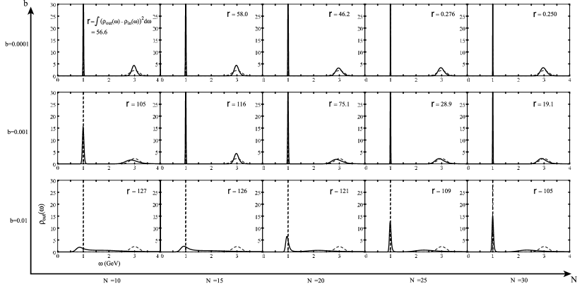
Figure 1: Input SPF with two Gaussian peaks (the dashed lines) and output SPF obtained by MEM (the solid lines) for different values of data-points $N$ and noise level $b$.

In Fig.2, the probability distribution $P[\alpha|DHm]$ (with an approximation discussed in Step 2 in Section 3.3) used to obtain the final image is shown for three different combinations of $N$ and $b$. The distribution tends to become peaked as $N$ increases and $b$ decreases.

Figure 2: Probability distribution $P[\alpha|DHm]$ for three different sets of $(N,b)$ in the case of Schematic SPF.

4.2 Realistic SPF

As an example of realistic spectral functions, we study SPF in the charged $\rho$-meson channel. The isospin symmetry relates it to the $e^{+}e^{-}$ annihilation data into hadrons in the isospin 1 channel. We take a relativistic Breit-Wigner form as a parametrization of SPF in this channel [7]:

$$\rho_{in}(\omega)={2\over\pi}\left[{F_{\rho}^{2}}{\Gamma_{\rho}m_{\rho}\over(\omega^{2}-m_{\rho}^{2})^{2}+\Gamma_{\rho}^{2}m_{\rho}^{2}}+{1\over 8\pi}\left(1+{\alpha_{s}\over\pi}\right){1\over 1+e^{(\omega_{0}-\omega)/\delta}}\right].$$ (4.5)

The pole residue $F_{\rho}$ is defined:

$$\langle 0|\bar{d}\gamma_{\mu}u|\rho\rangle=\sqrt{2}F_{\rho}m_{\rho}\epsilon_{\mu}\equiv\sqrt{2}f_{\rho}m_{\rho}^{2}\epsilon_{\mu},$$ (4.6)

where $\epsilon_{\mu}$ is the polarization vector. In the vector dominance model, the dimensionless residue $f_{\rho}$ is related to the $\rho\pi\pi$ coupling $g_{\rho\pi\pi}$ as $f_{\rho}=1/g_{\rho\pi\pi}$.

To get the correct threshold behavior due to the $\rho\rightarrow\pi\pi$ decay, we take the following energy-dependent width:

$$\Gamma_{\rho}(\omega)={g_{\rho\pi\pi}^{2}\over 48\pi}\ m_{\rho}\left(1-{4m_{\pi}^{2}\over\omega^{2}}\right)^{3/2}\ \theta(\omega-2m_{\pi}).$$ (4.7)

The empirical values of the parameters are

$$m_{\rho} = 0.77\ {\rm GeV},\ \ m_{\pi}=0.14\ {\rm GeV},$$

$$g_{\rho\pi\pi} = 5.45,$$ (4.8)

$$\omega_{0} = 1.3\ {\rm GeV},\ \ \delta=0.2\ {\rm GeV},$$

where we have assumed the vector dominance and $\alpha_{s}$ is taken to be 0.3 independent of $\omega$ for simplicity.

As for $m$, we take the form $m(\omega)=m_{0}\omega^{2}$ motivated by the asymptotic behavior of $\rho_{in}(\omega)$ in (4.5). $m_{0}$ is chosen to be 0.0257, which is slightly smaller than 0.0277 expected from the large $\omega$ limit of (4.5), $\rho_{in}(\omega\rightarrow\infty)=(2/\pi)(1/8\pi)(1+\alpha_{s}/\pi)$. The same parameters as those for the schematic SPF are chosen: $\omega_{max}=6$ GeV, $\Delta\omega=10$ MeV, $\tau_{min}=\Delta\tau=0.085$ fm. $N=\tau_{max}/\Delta\tau$ and $b$ are changed within the intervals, $10\leq N\leq 30$ and $0.0001\leq b\leq 0.01$.

In Fig.3, the mock data $D_{mock}(\tau_{i})$ obtained from (4.1) and (4.5) are shown for the noise parameter $b=0.001$. The linear slope of ${\rm log}D_{mock}(\tau_{i})$ for large $\tau_{i}$ is dictated by the lowest resonance, while the deviation from the linear slope for small $\tau_{i}$ originates from the continuum in SPF.

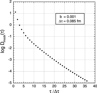
Figure 3: Mock data $D_{mock}(\tau_{i})$ in the case of the realistic SPF with Gaussian error attached.

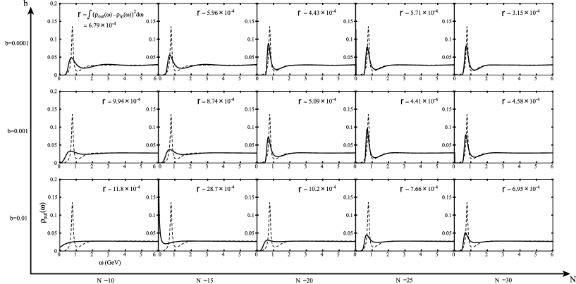
Figure 4: Input SPF with a resonance + continuum (the dashed lines) and output SPF obtained by MEM (the solid lines) for different values of $N$ and $b$.

In Fig.4, a comparison of $\rho_{out}(\omega)$ (the solid line) and $\rho_{in}(\omega)$ (the dashed line) is shown for various combinations of $N$ and $b$. The distance $r$ defined in (4.3) is also shown in the figure. Increasing $N$ and reducing the noise level $b$ lead to better SPFs closer to the input SPF as is evident from the figure as in the case of the schematic SPF.

In Fig.5, the probability distribution $P[\alpha|DHm]$ (with an approximation discussed in Step 2 in Section 3.3) used to obtain the final image is shown for three different combinations of $N$ and $b$. The narrower distribution is obtained when the data quality is better.

Figure 5: Probability distribution $P[\alpha|DHm]$ for three different sets of $(N,b)$ in the case of the realistic SPF.

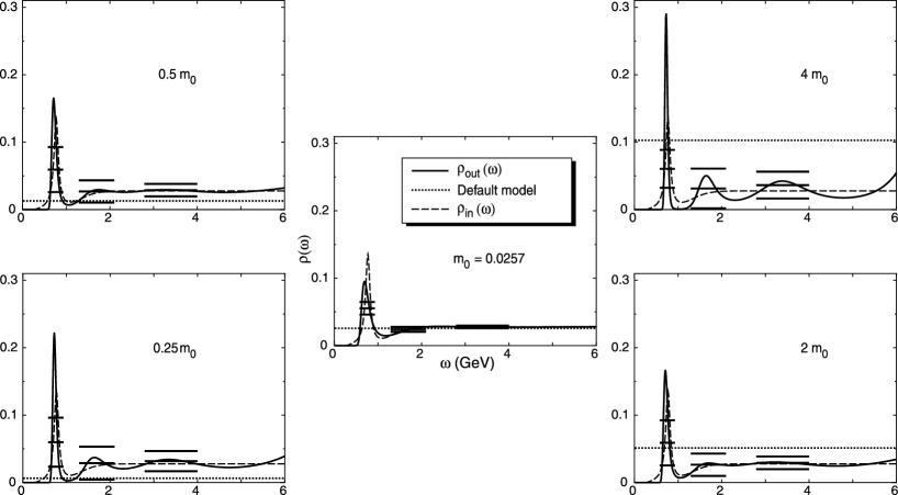
Figure 6: Default model dependence of the output image $\rho_{out}(\omega)$ (solid lines) for $N=25$ and $b=0.001$. The input images and the default models are shown by the dashed and dotted lines, respectively. Error bars for three different frequency regions are also attached. The middle figure is the same as that in Fig.4.

Finally, to see the sensitivity of the results against the change of $m_{0}$, $\rho_{out}(\omega)$ is shown in Fig.6 for five different values of the default model together with the error bars. $N=25$ and $b=0.001$ are chosen. Short dashed and long dashed lines correspond to the default model and the input SPF, respectively. The solid lines show the output image after the MEM analysis. $m_{0}=0.257$ is chosen in the middle figure which is the same with that in Fig.4, while the other four figures correspond to the default models for $0.25m_{0}$, $0.5m_{0}$, $2m_{0}$ and $4m_{0}$. Even under the factor 4 variation of the default model, the resultant SPFs show the peak + continuum structure. However, as the default model deviates from the expected asymptotic value, the SPF starts to have a “ringing” behavior.

Now, the error analysis discussed in Step 3 in Section 3.3 can tell us whether the ringing structure seen, e.g., in the $4m_{0}$ case (the upper right figure) corresponds to a real resonance or is the artifact of the maximum entropy method. The horizontal position and length of the bars in Fig.6 indicate the frequency region over which the SPF is averaged, while the vertical height of the bars denotes the uncertainty in the averaged value of the SPF in the interval. Implications of the error bars in Fig.6 are twofold; (i) the ringing images for $4m_{0}$ and $0.25m_{0}$ are statistically not significant, and (ii) the combination of the best SPF and the best default model may be selected by estimating the error bars (Step 4 in Section 3.3). In the present case, for the given data, the middle figure should be chosen to be the best one.

5 Analysis with lattice QCD data

5.1 Lattice basics

In lattice gauge theories [38], the Euclidean space-time is discretized into cells. In our simulations, we use an isotropic hypercubic grid, namely the lattice spacing $a$ is the same in all directions. In the following, we assume that the gauge group is SU(3) with QCD in mind. The fermion field $\psi(x)$ is defined at grid sites, while the gluon field is defined on links connecting adjacent pairs of grid sites (Fig.7). On the links connecting $x$ to $x\pm\hat{\mu}$ ($|\hat{\mu}|=a$), we define $U_{\pm\mu}(x)$ as

$$U_{\mu}(x)=\exp\left[iagA_{\mu}(x)\right],\ \ \ U_{-\mu}(x)=\exp\left[-iagA_{\mu}(x-\hat{\mu})\right].$$ (5.1)

$U_{\mu}(x)$ is an element of the SU(3) group, $g$ is the gauge coupling constant, and $A_{\mu}$ is the gauge field. The local gauge transformation for $\psi(x)$ and $U_{\mu}(x)$ on the lattice reads

$$\psi(x) \rightarrow V(x)\psi(x),\ \ \ \bar{\psi}(x)\rightarrow\bar{\psi}(x)V^{{\dagger}}(x),$$

$$U_{\mu}(x) \rightarrow V(x+\hat{\mu})U_{\mu}(x)V^{{\dagger}}(x),$$ (5.2)

where $V(x)$ is an SU(3) matrix defined at each site $x$.

Figure 7: Lattice variables. Quarks (gluons) are defined at the sites (on the links).

Using the plaquette variable defined by

$$W(x,\hat{\mu},\hat{\nu})=U_{-\nu}(x+\hat{\nu})U_{-\mu}(x+\hat{\mu}+\hat{\nu})U_{\nu}(x+\hat{\mu})U_{\mu}(x),$$ (5.3)

the single plaquette gluon action is written as

$$S_{p}=\beta_{lat}\sum_{x}\sum_{\mu<\nu}{\rm Re}\,{\rm Tr}\,\frac{1}{3}\left(1-W(x,\hat{\mu},\hat{\nu})\right),\ \ \ {\rm with}\ \ \beta_{lat}={6\over g^{2}}.$$ (5.4)

In the naive continuum limit $a\rightarrow 0$, $S_{p}$ approaches the continuum gauge action

$$S_{cont}=\frac{1}{4}\int d^{4}x(F_{\mu\nu}^{a}(x))^{2}.$$ (5.5)

For fermions, we use the Wilson quark action $S_{w}$ defined by

$$S_{w} = \sum_{x,y}\bar{\psi}(x)\left[\delta_{xy}-\kappa\sum_{{\mu}}\delta_{x,y+\hat{\mu}}(1+\gamma_{\mu})U_{\mu}(y)\right]\psi(y)$$ (5.6)

$$\equiv \sum_{x,y}\bar{\psi}(x)D_{w}(x,y;U)\psi(y).$$

Here the flavor indices for fermions are suppressed. $\gamma_{\mu}$ satisfies $\{\gamma_{\mu},\gamma_{\nu}\}=2\delta_{\mu\nu}$. $\Sigma_{\mu}$ is taken for both positive and negative directions of $\mu$ together with a convention $\gamma_{-\mu}=-\gamma_{\mu}$. $\kappa$ denotes the hopping parameter, while the quark mass $m_{q}$ is defined as

$$m_{q}a=\frac{1}{2\kappa}-\frac{1}{2\kappa_{c}(\beta_{lat})},$$ (5.7)

for a fixed $\beta_{lat}$. Here $\kappa_{c}(\beta_{lat})$ is the critical hopping parameter, at which the pion becomes massless.

The action for the whole system $S_{lat}$ is given by the sum of $S_{p}$ and $S_{w}$,

$$S_{lat}=S_{p}+S_{w}.$$ (5.8)

The expectation value of a physical observable ${\cal O}[U,\psi,\bar{\psi}]$ is given in terms of path integrals over the link variables $U_{\mu}(x)$ and fermion fields $\psi(x)$ and $\bar{\psi}(x)$,

$$\langle{\cal O}[U,\psi,\bar{\psi}]\rangle=\frac{1}{Z}\int[dUd\bar{\psi}d\psi]\ e^{-S_{lat}}\ {\cal O}[U,\psi,\bar{\psi}],$$ (5.9)

where $Z$ is given by

$$Z=\int[dUd\bar{\psi}d\psi]e^{-S_{lat}}=\int[dU]e^{-S_{p}}\ {\rm det}D_{w}(x,y;U).$$ (5.10)

In the quenched approximation, ${\rm det}D_{w}(x,y;U)$ is set to 1. Physically, this corresponds to ignoring the effect of virtual quark loops. This approximation simplifies numerical simulations by factor 1000 or so, since it is very time consuming to calculate the determinant of a huge matrix such as $D_{w}(x,y;U)$. In the quenched simulations, the first step is to generate an ensemble of gauge configurations $U_{\mu}(x)$ with the weight $e^{-S_{p}}$. A typical method for that purpose in SU(3) gauge theory is the pseudo heat-bath method combined with the over-relaxation method (for more details, see, e.g., [39]).

5.2 Lattice parameters

We take the open MILC code [40] with minor modifications and perform simulations with the single plaquette gluon action + Wilson quark action in the quenched approximation on a Hitachi SR2201 parallel computer at Japan Atomic Energy Research Institute. The basic lattice parameters in our simulations are

$${\rm coupling\ strength} \beta_{lat}={6\over g^{2}}=6.0,$$

$${\rm lattice\ size} N_{\sigma}^{3}\times N_{\tau}=20^{3}\times 24,$$

$${\rm hopping\ parameter} \kappa=0.153,\ 0.1545\ {\rm and}\ 0.1557.$$ (5.11)

The Dirichlet boundary condition (DB) in the temporal direction, which is defined by $U_{\mu}(x)=0$ for the last temporal links, is employed to have as many temporal data points as possible. In the spatial directions, the periodic (anti-periodic) boundary condition is used for the gluon (quark) as usual. Gauge configurations are generated by the pseudo heat-bath and over-relaxation algorithms with a ratio $1:4$. Each configuration is separated by 200 sweeps. The number of gauge configurations used in our analysis is $N_{conf}=161$.

We have also carried out simulations with the periodic (anti-periodic) boundary condition for the gluon (quark) in the temporal direction on the $20^{3}\times 24$ lattice with $\beta_{lat}=6.0$, and on the $40^{3}\times 30$ lattice with $\beta_{lat}=6.47$ on CP-PACS at Univ. of Tsukuba. Detailed MEM study in those cases will be reported elsewhere [41].

To calculate the two-point correlation functions, we adopt a point-source at $(\tau,\vec{x})=(0,\vec{0})$, and a point-sink at time $\tau$ with the spatial points averaged over the spatial lattice to extract physical states with vanishing three-momentum (see eq. (2.22)). The following local and flavor non-singlet operators are adopted for the simulations:

$${\rm scalar\ (S)}:\ \bar{d}u,\ \ \ \ \ \ \ \ \ {\mbox{pseudo-scalar}\ ({\rm PS})}:\ \bar{d}\gamma_{5}u,$$ (5.12)

$${\rm vector\ (V)}:\ \bar{d}\gamma_{\mu}u,\ \ \ \ \ {\mbox{axial-vector}\ ({\rm AV})}:\ \bar{d}\gamma_{\mu}\gamma_{5}u.$$ (5.13)

In the V and AV channels, the spin average is taken over the directions ${\mu}=1,2,3$ to increase statistics. Simulations for spin 1/2 and 3/2 baryons have been also carried out. Since special considerations are necessary for the decomposition of the SPFs in the baryon channels, we shall report the results in a separate publication [42].

Note here that the use of the point source and sink is essential for obtaining good signals for the resonance and continuum in the spectral function simultaneously. First of all, the SPF defined with the point source and sink for the vector channel is directly related to the experimental observables such as the $R$-ratio and the dilepton production rate as discussed in Section 2. Besides, there are two-fold disadvantages to use smeared sources and sinks in the MEM analysis: First of all, it is difficult to write down a simple sum rule such as eq.(2.22) for the smeared operators. Secondly, the coupling to the excited hadrons becomes small for such operators and one loses information on the higher resonances and continuum.

For the temporal data points to be used in the MEM analysis, we take $\tau_{min}/a=1$ and $\tau_{max}/a=12$. The latter is chosen to suppress the error from the Dirichlet boundary condition. In fact, we found that the statistical error of our data is well parametrized by formula (4.2) with a slope parameter $b$ up to $\tau/a=12$ and that the error starts to increase more rapidly above $\tau/a=12$.

5.3 Spectral functions and their asymptotic forms

We introduce the dimensionless SPFs, $\rho(\omega)$, as follows:

$$A_{{}_{S,PS}}(\omega)=\omega^{2}\rho_{{}_{S,PS}}(\omega),\ \ \ \ {1\over 3}\sum_{\mu=1,2,3}A^{\mu\mu}_{{}_{V,AV}}(\omega)=\omega^{2}\rho_{{}_{V,AV}}(\omega).$$ (5.14)

$\rho_{{}_{S,PS,V,AV}}(\omega)$ are defined in such a way that they approach finite constants when $\omega\rightarrow\infty$ in the continuum limit ($a\rightarrow 0$) as predicted by perturbative QCD (see eq.(2.15)).

Because of (2.8) and (2.9), we have

$$\rho_{{}_{S,PS,V,AV}}(\omega)=-\rho_{{}_{S,PS,V,AV}}(-\omega)\geq 0,\ \ \ \ {\rm with}~{}~{}\omega\geq 0.$$ (5.15)

The SPFs on the lattice in the chiral limit should have the following asymptotic form when $\omega$ is large and $a$ is small;

$$\rho_{j}(\omega\gg{\rm 1~{}GeV})={r_{1j}\over 4\pi^{2}}\left(1+r_{2j}{\alpha_{s}(\mu)\over\pi}\right)\left({1\over 2\kappa_{c}Z_{j}(\mu a)}\right)^{2},$$ (5.16)

where $j={\rm S,\ PS,\ V{\rm and}\ AV}$. The first two factors on the r.h.s. are the $q\bar{q}$ + $q\bar{q}g$ continuum expected from perturbative QCD. The third factor contains the non-perturbative renormalization constant, $Z_{j}(\mu a)$, of the lattice composite operator. The renormalization point $\mu$ should be chosen to be the typical scale of the system such as $1/a$.

$r_{1j}$ and $r_{2j}$ calculated perturbatively in the continuum QCD [43] are shown in Table 1. In [44], $Z_{j}(\mu a=1)$ in the chiral limit has been calculated numerically on the lattice with $\beta_{lat}=6.0$ for PB (the periodic (anti-periodic) boundary condition in the temporal direction for the gluon (quark)), which is summarized in Table 1. $Z_{j}$ for DB and those for PB are in principle different. This is because, in our simulation, the hadronic source is always on a time slice where DB is imposed and $Z_{j}$ detects the the boundary effect. Our measurement of the decay constant $f_{\rho}$ confirms this as shown later in section 5.5.1. Therefore, we use $Z_{j}$ listed in Table 1 only to guide our default model $m$.

$j$	$r_{1j}$	$r_{2j}$	$Z_{j}(\mu a=1)$	$\rho_{j}(\omega$=$\mu$=$1/a$)
S	${3/2}$	${11/3}$	0.77	0.80
PS	${3/2}$	${11/3}$	0.49	2.00
V	$1$	$1$	0.68	0.59
AV	$1$	$1$	0.78	0.45

Table 1: Constants for spectral functions in the asymptotic region. $r_{1j}$ and $r_{2j}$ are taken from [43]. $Z_{j}(\mu a=1)$ for $\beta_{lat}=6.0$ in the chiral limit $\kappa_{c}=0.1572$ is taken from [44], where PB is used in the temporal direction. For the estimates in the last column, we use $\alpha_{s}(\mu\simeq 2{\rm~{}GeV})=0.3$ [45], $\kappa_{c}=0.1572$ and $a^{-1}\sim~{}2$ GeV for $\beta_{lat}=6.0$.

So far we have assumed that the spatial momentum ${\bf k}$ vanishes due to the spatial integration on the lattice. However, it is not exactly the case for any finite set of gauge configurations. In most cases, the finite ${\bf k}$ error is harmless as far as ${\bf k}$ is small enough. However, it is potentially dangerous in the AV channel, where the SPF for finite $k^{\mu}=(\omega,{\bf k})$ is written as

$$A_{{\mu}{\nu}}(\omega,{\bf k})=(k_{\mu}k_{\nu}-k^{2}g_{\mu\nu})\ \rho_{{}_{T}}(\omega,{\bf k})+k_{\mu}k_{\nu}\ \rho_{{}_{L}}(\omega,{\bf k}).$$ (5.17)

Here $\rho_{{}_{T}}$ is the transverse spectral function, which does not have contamination from the pion pole. When ${\bf k}=0$, $\rho_{{}_{T}}$ reduces to $\rho_{{}_{AV}}(\omega\geq 0)\geq 0$ defined in (5.14). On the other hand, $\rho_{{}_{L}}$ is the longitudinal spectral function, which contains the pion pole: $\rho_{{}_{L}}(\omega,{\bf k})=2f_{\pi}^{2}\delta(k^{2}-m_{\pi}^{2})+\cdot\cdot\cdot$ with $f_{\pi}$ being the pion decay constant. Then, if small amount of ${\bf k}$ remains, there is possible contamination from the low-mass pion pole to the spin-averaged SPF:

$${1\over 3}\sum_{\mu=1,2,3}A_{\mu\nu}(\omega,{\bf k}\simeq 0)\simeq\omega^{2}\rho_{{}_{AV}}(\omega)+{\bf k}^{2}\rho_{{}_{L}}(\omega).$$ (5.18)

In the actual lattice data, this effect appears in $D({\tau})$ for large $\tau$. A possible way to subtract the contamination of $\rho_{{}_{L}}$ is to carry out the measurement with finite ${\bf k}$.

5.4 Discretization in $\omega$ space

In the MEM analysis, we need to discretize the $\omega$-space into pixels of an equal size $\Delta\omega$ and carry out the integration, (2.22), approximately. The upper limit of $\Delta\omega$ is determined by the requirement that the discretization error of the kernel $K$ in (2.22) is small enough, namely, $\tau\cdot\Delta\omega\ll 1$, which reads

$$\Delta\omega\ll{1\over\tau_{max}}<{1\over\tau}.$$ (5.19)

Thus $\tau_{max}^{-1}=(N_{\tau}a)^{-1}=(24a)^{-1}\sim 90{\rm MeV}$ is the upper bound of $\Delta\omega$ on our lattice.

Also, to obtain the good resolution of SPF, one needs to have small enough $\Delta\omega$ so that $|A_{l+1}-A_{l}|/|A_{l+1}+A_{l}|\ll 1$. In the maximum entropy method with singular value decomposition, there is no problem in choosing an arbitrary small value for $\Delta\omega$. In fact, as we have explained, the maximum search of $Q$ is always limited in the $N_{s}$ dimensional singular space, and $N_{s}$ is independent of $N_{\omega}$. Therefore, increasing $N_{\omega}$ or decreasing $\Delta\omega$ does not cause any numerical difficulty. In the following, we adopt $\Delta\omega=9.5$ MeV, which satisfies (5.19) and simultaneously gives a good resolution to detect sharp peaks in the spectral function.

Aside from $\Delta\omega$, we also need to choose the upper limit for the $\omega$ integration, $\omega_{max}$. Since this quantity should be comparable to or larger than the maximum available momentum on the lattice, we choose $\omega_{max}=7.1~{}{\rm GeV}>\pi/a\sim 6.9$ GeV. We have checked that larger values of $\omega_{max}$ do not change the result of $A(\omega)$ substantially, while smaller values of $\omega_{max}$ distort the high energy end of the spectrum. The dimension of the image to be reconstructed is $N_{\omega}\equiv\omega_{max}/\Delta\omega\sim 750$, which is in fact much larger than the maximum number of data points, $N=24$, available on our lattice.

5.5 Results of MEM analysis

5.5.1 Pseudo-scalar and vector channels

Let us first consider the PS and V channels. The lattice data $D(\tau_{i})$ in these channels are shown in Fig.8. For the MEM analysis, we take the formula (2.22) with $\beta=1/T=\infty$, since we use DB (the Dirichlet boundary condition). Also, $\tau_{min}/a=1$ has been taken to utilize the information available on the lattice as much as possible, while $\tau_{max}/a=12$ has been chosen to suppress errors caused by DB as discussed in the previous section.

Shown in Figs.9(a) and 9(b) are the reconstructed SPFs in these channels for different values of $\kappa$. $\omega_{max}$ is taken to be 7.1 GeV and $\Delta\omega=9.5$ MeV. We have used $m=m_{0}\omega^{2}$ with $m_{0}=2.0~{}(0.6)$ for the PS (V) channel motivated by the perturbative estimate $m_{0}\sim\rho(\omega\gg 1{\rm~{}GeV})$ in eq.(5.16) with Table 1. The sensitivity of the reconstructed SPFs on the variation of $m_{0}$ will be discussed later.

Spectral functions thus obtained in the PS and V channels shown in Figs.9a and 9b have a common structure: a sharp peak at low-energy, a less pronounced second peak, and a broad bump at high-energy. Let us discuss those structures in detail below.

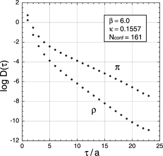
Figure 8: Lattice data $D(\tau_{i})$ in the PS and V channels with statistical errors.

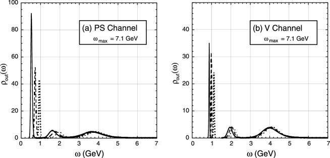
Figure 9: Reconstructed image $\rho_{out}(\omega)$ for the PS (a) and V (b) channels. The solid, dashed and dash-dotted lines are for $\kappa=$ 0.1557, 0.1545 and 0.153, respectively. For the PS (V) channel, $m_{0}$ is taken to be 2.0 (0.60). $\omega_{max}$ is 7.1 GeV.

1. To make sure that the lowest peak for each $\kappa$ in the PS (V) channel corresponds to the pion (the $\rho$-meson), we extract $m_{\pi}$ and $m_{\rho}$ in the chiral limit with the following procedure. First we fit the lowest peak by a Gaussian form and extract the position of the peak. Then, the linear chiral extrapolation is made for $(m_{\pi}a)^{2}$ and $m_{\rho}a$. The results together with $a$ using the input $m_{\rho}=0.77$ GeV are summarized in the column “MEM continuum kernel” in Table 2. They are consistent with those determined from the standard analysis using the asymptotic behavior of $D(\tau_{i})$ in the interval $10\leq\tau_{i}/a\leq 15$, which are shown in Table 2 in the column “asymptotic analysis”. Also, our results are consistent with those from the asymptotic behavior of $D(\tau)$ obtained by the QCDPAX Collaboration on a $24^{3}\times 54$ lattice with $\beta_{lat}=6.0$ [46]. They give $\kappa_{c}=0.1571$, $m_{\rho}a=0.331(22)$ and $a^{-1}=2.33(15)$ GeV.

   Although it is quite certain that the lowest peaks for each $\kappa$ in Figs.9(a) and 9(b) correspond to $\pi$ and $\rho$, the widths of these peaks in the quenched approximation do not have physical meaning, since they are artifact caused by the incompleteness of the information contained in lattice data. Nevertheless, the integrated strength of the peak corresponds to the physical decay constant of the mesons. For example, the dimensionless decay constant $f_{\rho}$ defined in eq.(4.6) is related to the lattice matrix element as

   $$\langle 0|(\bar{d}\gamma_{\mu}u)_{lat}|\rho({\bf k}=0)\rangle=\sqrt{2}\epsilon_{\mu}f_{\rho}m_{\rho}^{2}{1\over 2\kappa Z_{V}}.$$ (5.20)

   Therefore, it is further related to the spectral integral near the resonance as

   $$\int_{pole}\rho_{{}_{V}}(\omega)d\omega^{2}=2f_{\rho}^{2}m_{\rho}^{2}\ \left({1\over 2\kappa Z_{V}}\right)^{2},$$ (5.21)

   where the suffix “$pole$” implies the integral over the lowest isolated peak. This integral can be carried out numerically for each $\kappa$, and the linear extrapolation to the chiral limit has been done. The result for $f_{\rho}/Z_{V}$ is given in the 2nd row of Table 2 together with that obtained from the asymptotic analysis. The agreement is satisfactory. As we have mentioned before, $Z_{V}$ in the DB case is not necessary equal to that in the PB case. Therefore, we cannot predict $f_{\rho}$ from our data alone. Instead, we extract $Z_{V}$ in the DB case by comparing our measurement of $f_{\rho}/Z_{V}$ with experimental value of $f_{\rho}$. This leads to $Z_{V}^{DB}\simeq 0.38<Z_{V}^{PB}\simeq 0.68$. If we can have larger lattice and can place the hadronic source and sink far from the boundary, the difference between $Z_{j}^{DB}$ and $Z_{j}^{PB}$ should become small.

2. As for the second peaks in the PS and V channels, the results of the error analysis, which are shown in Fig.10, indicate that their spectral “shape” does not have much statistical significance, although the existence of the non-vanishing spectral strength is significant. With this reservation, we fit the position of the second peaks and make linear extrapolation to the chiral limit. The results are summarized in the 3rd row of Table 2 together with the experimental values. Since there exist two excited-$\rho$ experimentally observed, $\rho(1450)$ and $\rho(1700)$, we quote both values for $m_{\rho^{\prime}}/m_{\rho}$ in Table 2.

   One should note here that, in the standard two-mass fit of $D(\tau)$, the mass of the second resonance is highly sensitive to the lower limit of the fitting range, e.g., $m^{2nd}/m_{\rho}=2.21(27)~{}(1.58(26))$ for $\tau_{min}/a=8~{}(9)$ in the V channel with $\beta_{lat}=6.0$ [46]. This is because the contamination from the short distance contributions, which dominates the correlators at $\tau<\tau_{min}$, is not under control in such an approach. On the other hand, MEM does not suffer from this difficulty and can utilize the full information down to $\tau_{min}/a=1$. Therefore, MEM opens up a possibility of systematic study of higher resonances with lattice QCD.

3. As for the third bumps in Fig.9, the spectral “shape” is statistically not significant as is discussed in conjunction with Fig.10. They should rather be considered to be a part of the perturbative continuum instead of a single resonance. Fig.9 and Fig.12 given later show that SPF decreases substantially above 6 GeV, namely MEM automatically detects the existence of the momentum cutoff on the lattice $\sim\pi/a$. It is expected that MEM with the data on finer lattices leads to larger ultraviolet cut-offs in the spectra. Our preliminary analysis on a finer lattice ($40^{3}\times 30$ lattice with $\beta_{lat}=6.47$) in fact indicates that this is the case [41].

	asymptotic analysis	MEM	MEM	Experiments
		continuum kernel	lattice kernel
	($10\leq\tau_{i}/a\leq 15$)	($1\leq\tau_{i}/a\leq 12$)	($1\leq\tau_{i}/a\leq 12$)
$\kappa_{c}$	0.1572(1)	0.1570(3)	0.1569(1)
$m_{\rho}a$	0.343(10)	0.348(15)	0.348(27)	$-$
$a^{-1}$ (GeV)	2.24(7)	2.21(10)	2.21(17)
$f_{\rho}/Z_{V}$	0.48(3)	0.520(6)	$-$	$f_{\rho}=$0.198(5)
$m_{\pi^{\prime}}/m_{\rho}$	$-$	1.88(8)	1.74(8)	1.69(13)
$m_{\rho^{\prime}}/m_{\rho}$	$-$	2.44(11)	2.25(10)	1.90(3)  or  2.21(3)

Table 2: A comparison of the MEM analysis and the asymptotic analysis of the same lattice data obtained on the $20^{3}\times 24$ lattice with $\beta_{lat}=6.0$. The experimental value of $f_{\rho}$ obtained from the decay $\rho\rightarrow e^{+}e^{-}$ and the masses of $\rho^{\prime}$ and $\pi^{\prime}$ are also shown [45].

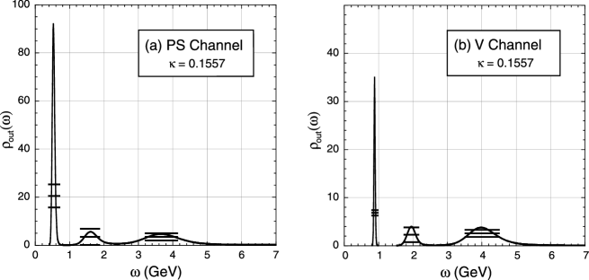
Figure 10: $\rho_{out}(\omega)$ in the V and PS channels for $\kappa=$ 0.1557 with error attached. $\omega_{max}=7.1$ GeV.

In Fig.10, we show the MEM images in the V and PS channels for $\kappa=0.1557$ with errors obtained in the procedure discussed in Step 3 in Section 3.3. The meanings of the error bars are the same as those in Fig.6. Namely, the horizontal position and length of the bars indicate the frequency region over which the SPF is averaged, while the vertical height of the bars denotes the uncertainty in the averaged value of the SPF in the interval.

The small error for the lowest peak in Fig.10 supports our identification of the peak with $\rho$. Although the existence of the non-vanishing spectral strength of the 2nd peak and 3rd bump is statistically significant, their spectral “shape” is either marginal or insignificant. Lattice data with better quality are called for to obtain better SPFs.

Figure 11: $P[\alpha|DHm]$ for the PS and V channels.

In Fig.11, $P[\alpha|DHm]$ (with the approximation discussed in Step 2 in Section 3.3) is shown for the PS and V channels in the case of $\kappa=0.1557$. We have found that the SPFs obtained after averaging over $\alpha$ and those at $\alpha=\hat{\alpha}$ have negligible difference although the distribution of $\alpha$ spreads over the range $0\rightarrow 1$ in Fig.11.

The sensitivity of the results under the variation of $\omega_{max}$ is shown in Fig.12, where $\omega_{max}=8.5$ GeV is adopted. Comparison of Fig.12 and Fig.9 shows no appreciable change of SPFs under the variation of $\omega_{max}$ as long as $\omega_{max}\geq\pi/a$.

We have also checked that the result is not sensitive, within the statistical significance of the image, to the variation of $m_{0}$ by factor 5 as shown in Fig.13. The default model dependence is relatively weak compared to the case of the mock data shown in Fig.6 partly because the off-diagonal components of the covariance matrix for the lattice data are not negligible and stabilize the final images.

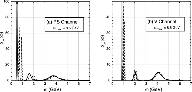
Figure 12: SPFs in the V and PS channels for $\omega_{max}=8.5$ GeV. The solid, dashed and dash-dotted lines are for $\kappa=$ 0.1557, 0.1545 and 0.153, respectively.

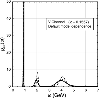
Figure 13: The default model dependence of the output image in the vector channel for $\omega_{max}=7.1$ GeV. The solid line corresponds to $m_{0}=0.6$ (the same value with that taken in Fig.9 and Fig.10, while the long (short) dashed line corresponds to $5m_{0}$ ($m_{0}/5$).

5.5.2 Scalar and axial-vector channels

In Fig.14, the spectral functions for the S and AV channels are shown. In those channels, we have used $\tau_{max}/a=12~{}(10)$ for the S (AV) channel. Smaller $\tau_{max}$ is chosen in the AV channel to avoid the pion contamination that contributes to the correlator at large $\tau$ as discussed in Section 5.3. Although the peak + continuum structure is seen in Fig.14, SPF does not change in a regular way under the variation of the quark mass, which prevents us from making chiral extrapolation of the peaks. More statistics and also better technique are needed to obtain SPFs with good quality in these channels.

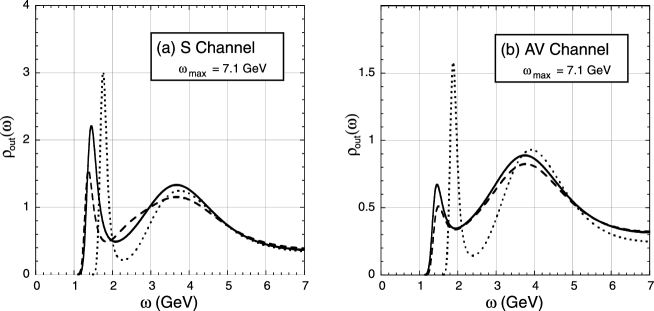
Figure 14: SPF for S and AV channels. The solid, dashed and dash-dotted lines are for $\kappa=$ 0.1557, 0.1545 and 0.153, respectively.

5.5.3 Lattice versus continuum kernel

In the MEM analysis presented so far, we have relied on the spectral representation derived in the continuum limit,

$$D(\tau)=\int_{0}^{\infty}\ K(\tau,\omega)\ A(\omega)\ d\omega.$$ (5.22)

Here the kernel $K$ at $T=0$ is related to the free boson propagator with a mass $\omega$:

$$K(\tau,\omega)=e^{-\omega\tau}=2\omega\int_{-\infty}^{+\infty}{d\nu\over 2\pi}{e^{i\nu\tau}\over\omega^{2}+\nu^{2}}.$$ (5.23)

Now, to study the systematic error from the finite lattice spacing in extracting SPF, one may artificially define a “lattice spectral representation” as

$$D(\tau)=\int_{0}^{\infty}\ K^{lat}(\tau,\omega)\ A^{lat}(\omega)\ d\omega,$$ (5.24)

where $K^{lat}$ is a “lattice kernel” at $T=0$ defined through the lattice boson propagator with a mass $\omega$:

$$K^{lat}(\tau,\omega;a)=2\omega\int_{-\pi/a}^{+\pi/a}{d\nu\over 2\pi}{e^{i\nu\tau}\over\omega^{2}+({2\over a}\sin{\nu a\over 2})^{2}}.$$ (5.25)

$K^{lat}$ and $A^{lat}$ approach $K$ and $A$, respectively, in the continuum limit. Therefore, by taking the same lattice data $D(\tau)$ on the l.h.s. of (5.22) and (5.24) and by comparing the resultant $A(\omega)$ and $A^{lat}(\omega)$ in the MEM analysis, one can estimate a part of the systematic error from the finiteness of the lattice spacing.

The difference of $K^{lat}$ and $K$ becomes substantial for large $\tau\omega$, which is shown in Fig.15. Therefore, the finite $a$ error appears typically at large $\omega$. The spectral functions in the V and PS channels obtained with the lattice kernel are shown in Fig.16. In Table 2, the masses extrapolated to the chiral limit are shown in the column “MEM lattice kernel”. ($f_{\rho}$ is not shown in the table, since it is difficult to isolate the $\rho$-pole unambiguously from Fig.16.) The results are consistent with those of “MEM continuum kernel” within error bars. In Fig.17, the SPFs with error attached are shown for the PS and V channels. Taking into account those errors, it is hard to distinguish the images obtained by $K$ and $K^{lat}$ with the present lattice data, although the SPFs in Fig.17 are flat compared with those in Fig.10.

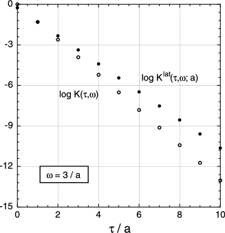
Figure 15: Comparison of the lattice kernel $K^{lat}$ and the continuum kernel $K$ near the highest frequency on the lattice $\omega=3/a$.

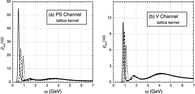
Figure 16: SPFs for the V and PS channels obtained with the lattice kernel. The solid, dashed and dash-dotted lines are for $\kappa=$ 0.1557, 0.1545 and 0.153, respectively.

Figure 17: SPFs for the V and PS channels obtained with the lattice kernel with error attached for $\kappa=0.1557$.

6 Summary and concluding remarks

In this article, we have examined the spectral function (SPF) in QCD and its derivation from the lattice QCD data. The maximum entropy method (MEM), which allows us to study SPFs without making a priori assumptions on the spectral shape, turns out to be quite successful and promising even for limited number of lattice QCD data with noise. In particular, the uniqueness of the solution and the quantitative error analysis make MEM superior to any other approaches adopted previously for studying SPFs on the lattice. Also, the singular value decomposition (SVD) of the kernel of the spectral sum rule leads to a very efficient algorithm for obtaining SPFs numerically.

By analyzing mock data, we have tested that the MEM image approaches the exact one as the number of temporal data points is increased and the statistical error of the data is reduced. Even with the lattice QCD data at $T=0$ obtained on the $20^{3}\times 24$ lattice with the lattice spacing $a\simeq 0.09$ fm, MEM was able to produce resonance peaks with correct masses and the continuum structure. The statistical significance of the obtained spectral functions has been also analyzed. Better data with smaller $a$ and larger lattice volume will be helpful for obtaining SPFs with smaller errors.

MEM introduces a new way of extracting physical information as much as possible from the lattice QCD data. Before ending this article, we list open problems for future studies. Some of them are straightforward and some of them require more work.

Technical issues:

• The number of temporal points $N$ and the lattice spacing $a$ are the crucial quantities for the MEM analysis to be successful. In this article, we have fixed $N=12$ and $a=0.09$ fm for extracting SPF from the lattice data. However, it is absolutely necessary to study $N$ and $a$ dependence of the resultant SPFs. For this purpose, we have collected 160 gauge configurations on CP-PACS at Univ. of Tsukuba with $40^{3}\times 30$ lattice and $\beta_{lat}=6.47$ ($a\sim 0.05$ fm) with the periodic boundary condition. The detailed MEM analysis of the data will be reported elsewhere [41].

• We have made chiral extrapolation only for the peaks of SPFs but not for the whole spectral structure in this article: In fact we have found that neither the direct extrapolation of the MEM image $A_{out}(\omega)$ nor the extrapolation of $D(\tau)$ and $C$ works in a straightforward manner. This is an open problem for future study.

• Although we have shown that one can select an optimal default model by varying $m(\omega)$ and estimating the errors of SPFs, the variation was within an assumed functional form such as $m(\omega)=m_{0}\omega^{n}$ motivated by the asymptotic behavior of the spectral functions in QCD. How to optimize the default model given data in a systematic way should be studied further. (For a possible procedure by estimating $P[m|DH]$, see ref.[22].)

Physics issues:

• Further studies on the scalar and axial-vector channels are necessary to explore the applicability of MEM for not-so-clean lattice-data.

• MEM analysis for baryons is quite useful in extracting information on excited baryons and their chiral structure [42].

• Applications to heavy resonances such as the glueballs, and charmed/bottomed hadrons will be an ideal place for MEM, since one can extract ground state peaks with limited number of data points obtained at relatively short distances. For the study of charmonium on $40^{3}\times 30$ lattice with $\beta_{lat}=6.47$, see [41].

• When one studies a two-point correlation function of operators ${\cal O}_{1}$ and ${\cal O}_{2}$ with ${\cal O}_{1}\neq{\cal O}_{2}$, one encounters SPF which is not necessarily positive semi-definite. Typical examples are the meson and baryon mixings such as $\rho$-$\omega$, $\pi^{0}$-$\eta$, $\eta$-$\eta^{\prime}$, glueball-$q\bar{q}$ and $\Lambda$-$\Sigma^{0}$ (see e.g. [47]). The generalization of the Shannon-Jaynes entropy to non positive-definite images is possible [48], and it is an interesting future problem to study hadron mixings from the generalized MEM.

• Full QCD simulations combined with MEM may open up a possibility of first principle determination of resonance widths such as $\rho(770)\rightarrow 2\pi$, $\sigma(400-1200)\rightarrow 2\pi$ and $a_{1}(1260)\rightarrow 3\pi$. Also it serves for unraveling the structure of the mysterious scalar meson “$\sigma$” [49].

• The long-standing problem of in-medium spectral functions of vector mesons ($\rho$, $\omega$, $\phi$, $J/\psi$, $\Upsilon$, $\cdots$, etc ) and scalar/pseudo-scalar mesons ($\sigma$, $\pi$, $\cdots$, etc.) can be studied using MEM combined with finite $T$ lattice simulations. The in-medium behavior of the light vector mesons [5, 10, 28, 29, 50, 51] and scalar mesons [3, 52] is intimately related to the chiral restoration in hot/dense matter, while that of the heavy vector mesons is related to deconfinement [11, 53, 54]. An anisotropic lattice is necessary for this purpose to have enough data points in the temporal direction at finite $T$ [55]. (See also a recent attempt on the basis of NRQCD simulation [56].) Also, it is interesting to study SPFs with finite three-momentum ${\bf k}$, since $\omega$ and ${\bf k}$ enter in the in-medium SPFs as independent variables.

• Possible existence of non-perturbative collective modes above the critical temperature of the QCD phase transition speculated in [3, 57, 58] may also be studied efficiently by using MEM, since the method does not require any specific ansätze for the spectral shape. Also, correlations in the diquark channels in the vacuum and in medium are interesting to be explored in relation to the $q$-$q$ correlation in baryon spectroscopy and to color superconductivity at high baryon density [59].

Acknowledgements

We are grateful to MILC collaboration for providing us their open codes for lattice QCD simulations, which has enabled this research. Most of our simulations presented in this article were carried out on a Hitachi SR2201 parallel computer at Japan Atomic Energy Research Institute. We thank S. Chiba for giving us an opportunity to use the above computer. We also thank S. Aoki, K. Kanaya, A. Ukawa and T. Yoshie for their interests in this work and encouragements, and thank K. Sasaki for reading the manuscript carefully. T. H. thanks H. Feldmeier for the discussion on the uniqueness of the solution of MEM. M. A. (T. H.) was partly supported by Grant-in-Aid for Scientific Research No. 10740112 and No. 11640271 (No. 98360 and No.12640263) of the Japanese Ministry of Education, Science and Culture.

Appendix A Monkey argument for entropy and prior probability

Throughout Appendix A and B, we shall use the common notation $f(x)$ for the image instead of $A(\omega)$ used in the text.

What we need in the maximum entropy method is the prior probability $P(f\in V)$, namely, the probability that the image $f(x)$ is in a certain domain $V$. It can be generally written as

$$P(f\in V)={1\over Z_{S}(\alpha)}\int_{V}[df]\ \Phi(\alpha S(f)),$$ (A.1)

where $\alpha$ is an arbitrary constant defined for later use, and $Z_{S}(\alpha)$ is a normalization factor. We assume that $\Phi$ is a monotonic function of the would-be entropy $S(f)$, so that the most probable image $f$ is obtained as a stationary point of $S(f)$.

The so-called “monkey argument”, which is based on the law of large numbers, can determine the explicit form of $\Phi$ and $S(f)$ (see, e.g., [21, 31, 32, 33]). Here we shall recapitulate the essential part of this derivation.

Let us first discretize the basis space $x$ into $N$ cells. Correspondingly, $f(x)$ is discretized as $f_{i}$ $(1\leq i\leq N)$. Suppose a monkey throws $M$ balls. $M$ is assumed to be large. Define $n_{i}$ as the actual number of balls which the $i$-th cell received. Also, the $i$-th cell has a probability $p_{i}$ to receive a ball. Then $\lambda_{i}$ (the expectation value of the number of the balls in the $i$-th cell) reads $\lambda_{i}=Mp_{i}$ with $\sum_{i=1}^{N}\lambda_{i}=M$.

The probability that the $i$-th cell receives $n_{i}$ balls is given by the binomial distribution. Its large $M$ limit with $\lambda_{i}$ fixed is the Poisson distribution $P_{\lambda_{i}}(n_{i})$:

$$B_{M,\,p_{i}}(n_{i}) = \ \frac{M!}{n_{i}!(M-n_{i})!}\ p_{i}^{n_{i}}\ (1-p_{i})^{M-n_{i}}\rightarrow P_{\lambda_{i}}(n_{i})\ \ \ (M\rightarrow\infty).$$ (A.2)

Therefore, the probability that a certain image $\vec{n}=(n_{1},n_{2},\cdot\cdot\cdot,n_{N})$ is realized reads

$$P_{\vec{\lambda}}(\vec{n})=\prod_{i=1}^{N}P_{\lambda_{i}}(n_{i})=\prod_{i=1}^{N}\ {\lambda_{i}^{n_{i}}\ e^{-\lambda_{i}}\over n_{i}!},$$ (A.3)

where the normalization is given by $\sum_{n_{i}=0}^{\infty}P_{\lambda_{i}}(n_{i})=1$ $(i=1,2,\cdots,N)$.

Since $n_{i}$ may be large as $M$ is large, we introduce a small “quantum” $q$ and define the finite image $f_{i}$ and the default model $m_{i}$ as

$$f_{i}=qn_{i},\quad m_{i}=q\lambda_{i}.$$ (A.4)

In terms of (A.4), $P(f\in V)$ is written as

$$P(f\in V)=\sum_{\vec{n}\in V}P_{\vec{\lambda}}(\vec{n})\simeq\int_{V}{\prod_{i=1}^{N}df_{i}\over q^{N}}\ \prod_{i=1}^{N}{\lambda_{i}^{n_{i}}\ e^{-\lambda_{i}}\over n_{i}!}\simeq\int_{V}\prod_{i=1}^{N}{df_{i}\over\sqrt{f_{i}}}\ {e^{S(f)/q}\over(2\pi q)^{N/2}},$$ (A.5)

where small $q$ is assumed for converting the sum to the integral, and the Stirling’s formula, $n!\simeq\sqrt{2\pi n}e^{n\log n-n}$, is used to obtain the last expression.

$S(f)$ is nothing but the Shannon-Jaynes entropy,

$$S(f)=\sum_{i=1}^{N}\left[f_{i}-m_{i}-f_{i}\log\left({f_{i}\over m_{i}}\right)\right].$$ (A.6)

Comparing (A.5) with (A.1), one finds

$$q=\alpha^{-1},\ \ \ [df]=\prod_{i=1}^{N}\frac{df_{i}}{\sqrt{f_{i}}},\ \ \ Z_{S}(\alpha)=\left(\frac{2\pi}{\alpha}\right)^{N/2}.$$ (A.7)

Note also that the measure $M(f)$ defined by

$$M(f)=\prod_{i=1}^{N}{f_{i}}^{-1/2}$$ (A.8)

is rewritten as

$$M(f)=\sqrt{\det g}\ \ \ {\rm with}\ \ \ g_{ij}=(1/f_{i})\delta_{ij}=-{\partial^{2}S(f)\over\partial f_{i}\partial f_{j}}.$$ (A.9)

The metric tensor $-g_{ij}$ for the functional integral over $f$ is thus related to the curvature matrix of $S(f)$.

Appendix B Axiomatic construction of entropy

The axiomatic construction of the Shannon-Jaynes entropy $S$ given below is a modified version of that given in [34]. We have changed the statement of each axiom so that it becomes easier to understand the idea behind.

For positive semi-definite distribution $f(x)$, we want to assign a real number $S(f)$ (the Shannon-Jaynes entropy) as

$$f\mbox{ is a more plausible image than }g\ \ \leftrightarrow\ \ S(f)>S(g).$$ (B.10)

If there exists an external constraint on $f(x)$ such as $C(f(x))=0$, the most plausible image is given by the following condition

$$\delta_{f}\left[S(f)-\lambda C(f)\right]=0,$$ (B.11)

with $\lambda$ being a Lagrange multiplier. The explicit form of $S$ is uniquely fixed by the following axioms.

Axiom I: Locality

$S(f)$ is a local functional of $f(x)$ without derivatives. Namely, there is no correlation between the images at different $x$.

This leads to a form

$$S(f)=\int dx\ m(x)\ \theta(f(x),x).$$ (B.12)

Here $m(x)$ is a positive definite function which defines the integration measure. $\theta$ is an arbitrary local function of $f(x)$ and $x$ without derivatives acting on $f$.

Axiom II: Coordinate Invariance

$f(x)$ and $m(x)$ transform as scalar densities under the coordinate transformation $x^{\prime}=x^{\prime}(x)$, namely, $f(x)dx=f^{\prime}(x^{\prime})dx^{\prime}$ and $m(x)dx=m^{\prime}(x^{\prime})dx^{\prime}$. Also, $S$ is a scalar.

This axiom allows only two invariants for constructing $S$ in (B.12): $m(x)dx=m^{\prime}(x^{\prime})dx^{\prime}$ and $f(x)/m(x)=f^{\prime}(x^{\prime})/m^{\prime}(x^{\prime})$. Therefore,

$$S(f)=\int dx\ m(x)\ \phi(f(x)/m(x)).$$ (B.13)

Axiom III: System Independence

If $x$ and $y$ are two independent variables, the image $F(x,y)$ is written as a product form $F(x,y)=f(x)g(y)$ together with the integration measure $m(x,y)=m_{f}(x)m_{g}(y)$. Furthermore, the first variation of $S(F)$ with respect to $F(x,y)$ leads to an additive form with some functions $\alpha(x)$ and $\beta(y)$;

$${\delta S(F)\over\delta F(x,y)}=\alpha(x)+\beta(y).$$ (B.14)

From this axiom, images $f(x)$ and $g(y)$ are determined independently from the variational equation ${\delta S(F)/\delta F(x,y)}=0$. First of all, (B.13) reads

$$S(F)=\int dx\int dy\ m(x,y)\ \phi(F(x,y)/m(x,y)).$$ (B.15)

Acting the derivative $\partial^{2}/\partial x\partial y$ on eq.(B.14) with (B.15) and using $Z\equiv F(x,y)/m(x,y)=(f(x)/m_{f}(x))(g(y)/m_{g}(y))$, one obtains

$$Z{d^{2}\sigma(Z)\over dZ^{2}}+{d\sigma(Z)\over dZ}=0,$$ (B.16)

where $\sigma(Z)=d\phi(Z)/dZ$. The solution of this differential equation is $\sigma(Z)=c_{1}\log Z-c_{0}$, which leads, up to an irrelevant constant, to

$$\phi(Z)=c_{1}Z\log Z-(c_{0}+c_{1})Z.$$ (B.17)

Thus one arrives at

$$S(f)=\int dx\ m(x)\phi(f/m)=\int dx\ f(x)\left[c_{1}\log\left({f(x)\over m(x)}\right)-(c_{0}+c_{1})\right],$$ (B.18)

where we have dropped the suffix $f$ in $m_{f}(x)$ for simplicity. The curvature of $S$ is dictated by $c_{1}$, since $(\delta/\delta f)^{2}S(f)=c_{1}/f$ and $f\geq 0$. We choose $c_{1}=-1$ for having $S$ bounded from above and for overall normalization.

Axiom IV: Scaling

If there is no external constraint on $f(x)$, the initial measure is recovered after the variation, i.e., $f(x)=m(x)$.

This axiom leads to $c_{0}=0$ in (B.18), since the unconstrained solution of $\delta S(f)/\delta f=0$ is $f(x)=m(x)e^{c_{0}/c_{1}}$. Also, it is convenient to add a constant to $S(f)$ in (B.18) to make $S(f=m)=0$. Thus we arrive at

$$S(f)=\int dx\left[f(x)-m(x)-f(x)\log\left({f(x)\over m(x)}\right)\right],$$ (B.19)

which is the desired expression of the Shannon-Jaynes entropy.

Appendix C The singular value decomposition

Here we give a proof of the singular value decomposition (SVD) of a general $m\times n$ matrix $P$ following [36].

The singular values of a matrix $P$ are defined as the square root of the eigenvalues of $P^{\dagger}P$. By definition, $P^{\dagger}P$ is an $n\times n$ Hermitian matrix and has real and non-negative eigenvalues. We also define the norm of the vector $x\in{\bf C}^{n}$ and the spectral norm of the $m\times n$ matrix $P$, respectively, as

$$\parallel x\parallel_{2} = \left[\sum_{i=1}^{n}|x_{i}|^{2}\right]^{1/2},$$ (C.20)

$$\parallel P\parallel_{2} = \left[{\rm maximum\ eigenvalue\ of\ }P^{\dagger}P\right]^{1/2}$$ (C.21)

$$= \left[{\rm max}(x^{\dagger}P^{\dagger}Px)\right]^{1/2}\ \ (x\in{\bf C}^{n},\parallel x\parallel_{2}=1).$$ (C.22)

SVD Theorem:
Let $P$ be an $m\times n$ matrix ($m\geq n$), $U$ be an $m\times m$ unitary matrix, and $V$ be an $n\times n$ unitary matrix. Then, $P$ can be decomposed as

$$P=U\Xi V^{\dagger},$$ (C.23)

where $\Xi$ is an $m\times n$ diagonal matrix with the diagonal elements being the singular values of $P$, namely, $\Xi={\rm diag}(\xi_{1},\xi_{2},\cdots,\xi_{n})$ with $\xi_{1}\geq\xi_{2}\geq\cdots\geq\xi_{n}\geq 0$.

Proof:
Define the maximum singular value of $P$ as $\xi_{1}$. Then, there exists a vector $x_{1}$ which satisfies the relation: $\xi_{1}^{2}=(x_{1}^{\dagger}P^{\dagger}Px_{1})$. Also there exists a vector $y_{1}\in{\bf C}^{m}(\parallel y\parallel_{2}=1)$ with the property, $Px_{1}=\xi_{1}y_{1}$.

For $x_{1}$ and $y_{1}$ obtained above, one may introduce non-square matrices $U_{2}$ and $V_{2}$ such that $U_{1}$ and $V_{1}$ given below become an $m\times m$ unitary matrix and an $n\times n$ unitary matrix, respectively:

$$U_{1}=(y_{1},U_{2}),\ \ \ V_{1}=(x_{1},V_{2}).$$ (C.24)

Using $U_{1}$ and $V_{1}$ defined above, $P$ is transformed into $P_{1}$ as

$$P_{1}\equiv U_{1}^{\dagger}PV_{1}=\left(\begin{array}[]{c}y_{1}^{\dagger}\\ U_{2}^{\dagger}\end{array}\right)P(x_{1},V_{2})=\left(\begin{array}[]{cc}\xi_{1}&y_{1}^{\dagger}PV_{2}\\ 0&U_{2}^{\dagger}PV_{2}\\ \end{array}\right)\equiv\left(\begin{array}[]{cc}\xi_{1}&z_{1}^{\dagger}\\ 0&Q_{2}\\ \end{array}\right),$$ (C.31)

where $z_{1}\in{\bf C}^{n-1}$ and $Q_{2}$ being an $(m-1)\times(n-1)$ matrix.

Now, we show that $z_{1}$ is actually a null vector:

$$\xi_{1}^{2} = \parallel P\parallel_{2}^{2}=\parallel P_{1}\parallel_{2}^{2}={\rm max}(x^{\dagger}P_{1}^{\dagger}P_{1}x)$$

$$\geq {1\over\xi_{1}^{2}+\parallel z_{1}\parallel_{2}^{2}}\ (\xi_{1},z_{1}^{\dagger})P_{1}^{\dagger}P_{1}\left(\begin{array}[]{c}\xi_{1}\\ z_{1}\\ \end{array}\right)$$

$$= {1\over\xi_{1}^{2}+\parallel z_{1}\parallel_{2}^{2}}\left[(\xi_{1}^{2}+\parallel z_{1}\parallel_{2}^{2})^{2}+\parallel Q_{2}z_{1}\parallel_{2}^{2}\right]$$

$$\geq \xi_{1}^{2}+\parallel z_{1}\parallel_{2}^{2}.$$ (C.35)

Since $\xi_{1}$ is the maximum singular value of $P$ and $P_{1}$, $\xi_{2}$ defined as the maximum SV of $Q_{2}$ satisfies $\xi_{1}\geq\xi_{2}$. Applying the same procedure to $Q_{2}$, $Q_{3}$, $\cdots$, one finds

$$P_{n}=U^{\dagger}PV=\left(\begin{array}[]{ccc}\xi_{1}&&\\ &\ddots&\\ &&\xi_{n}\\ 0&\cdots&0\\ \end{array}\right)\equiv\Xi.$$ (C.40)

Thus one arrives at the singular value decomposition $P=U\Xi V^{\dagger}$. (QED)

One may neglect the irrelevant components of $U$ and $\Xi$ so that they are an $m\times n$ matrix and an $n\times n$ matrix, respectively. In this case, $U$ satisfies the condition $U^{\dagger}U=1$, while $V^{\dagger}V=VV^{\dagger}=1$. This form of SVD is used in the text.

References

- [1] M. A. Shifman, A. I. Vainshtein and V. I. Zakharov, Nucl. Phys. B147 (1979) 385, 448.
- [2] M. A. Shifman, Prog. Theor. Phys. Suppl. 131 (1998) 1.
- [3] T. Hatsuda and T. Kunihiro, Phys. Rev. Lett. 55 (1985) 158; Phys. Lett. B185 (1987) 304.
-
[4]
M. Dey, V. L. Eletsky and B. L. Ioffe, Phys. Lett. B252 (1990) 620.
C. Gale and J. Kapusta, Nucl. Phys. B357 (1991) 65.
S. H. Lee, C. Song and H. Yabu, Phys. Lett. B341 (1995) 407.
C. Song, P.W. Xia and C. M. Ko, Phys. Rev. C54 (1996) 3218. -
[5]
M. Asakawa and C. M. Ko, Phys. Rev. C 48 (1993) R526.
M. Herrmann, B. Friman and W. Nörenberg, Nucl. Phys. A560 (1993) 411.
B. Friman and H. J. Pirner, Nucl. Phys. A617 (1997) 496.
W. Peters, M. Post, H. Lenske, S. Leupold and U. Mosel, Nucl. Phys. A632 (1998) 109.
G. E. Brown, G. Q. Li, R. Rapp, M. Rho and J. Wambach, Acta Phys. Pol. B29 (1998) 2309.
D. Cabrera, E. Oset and M. J. Vicente Vacas, nucl-th/0011037. -
[6]
T. Hatsuda and T. Kunihiro, Phys. Rep. 247 (1994) 221.
G. E. Brown and M. Rho, Phys. Rep. 269 (1996) 333. - [7] E. V. Shuryak, Rev. Mod. Phys. 65 (1993) 1.
- [8] G. Agakichiev et al. (CERES Collaboration), Phys. Rev. Lett. 75 (1995) 1272; Phys. Lett. B422 (1998) 405.
- [9] M. C. Abreu et al. (NA50 Collaboration), Phys. Lett. B477 (2000) 28.
-
[10]
R. Rapp and J. Wambach, Adv. Nucl. Phys.
25 (2000) 1 (hep-ph/9909229).
J. Alam, S. Sarkar, P. Roy, T. Hatsuda and B. Sinha, Ann. Phys. (N.Y.), 286 (2000) 159 (hep-ph/9909267).
G. Chanfray, nucl-th/0012068. - [11] H. Satz, Rept. Prog. Phys. 63 (2000) 1511 (hep-ph/0007069).
- [12] Lattice 99 Proceedings, Nucl. Phys. B (Proc. Suppl.) 83 (2000) 1.
-
[13]
S. Aoki et al. (CP-PACS Collaboration), Phys. Rev. Lett. 84
(2000) 238.
S. Aoki, Lattice Calculations and Hadron Physics, eConf C990809 (2000) 657 (hep-ph/9912288).
K. Kanaya, Hadronic Properties from Lattice QCD with Dynamical Quarks, hep-ph/0005294. -
[14]
M. -C. Chu, J. M. Grandy, S. Huang and J. W. Negele,
Phys. Rev. D 48 (1993) 3340.
D. B. Leinweber, Phys. Rev. D 51 (1995) 6369.
D. Makovoz and G. A. Miller, Nucl. Phys. B468 (1996) 293.
C. Allton and S. Capitani, Nucl. Phys. B526 (1998) 463. -
[15]
T. Hashimoto, A. Nakamura and I. O. Stamatescu,
Nucl. Phys. B400 (1993) 267; ibid. B406 (1993) 325.
Ph. de Forcrand et al. (QCD-TARO Collaboration), hep-lat/0008005. -
[16]
Y. Nakahara, M. Asakawa and T. Hatsuda, Phys. Rev. D60
(Rapid Comm.) (1999) 091503 (hep-lat/9905034).
Y. Nakahara M. Asakawa and T. Hatsuda, Nucl. Phys. (Proc. Suppl.) 83 (2000) 191 (hep-lat/9909137). - [17] C. E. Shannon and W. Weaver, The Mathematical Theory of Communication, (Univ. of Illinois Press, Urbana, 1949).
- [18] E. T. Jaynes, Phys. Rev. 106 (1957) 620; ibid. 108 (1957) 171.
- [19] E.T. Jaynes, How does brain do plausible reasoning?, Stanford Univ. Microwave Lab. report 421 (1957), reprinted in Maximum-Entropy and Bayesian Methods in Science and Engineering, vol.1, pp.1-24, eds. G. J. Erickson and C. R. Smith, (Kluwer Academic Publishers, London, 1988).
- [20] B. R. Frieden, J. Opt. Soc. Am., 62 (1972) 511.
- [21] N. Wu, The Maximum Entropy Method, (Springer-Verlag, Berlin, 1997).
- [22] See a recent review, M. Jarrell and J. E. Gubernatis, Phys. Rep. 269 (1996) 133.
-
[23]
R. N. Silver et al., Phys. Rev. Lett. 65 (1990) 496.
R. N. Silver et al., Phys. Rev. B41 (1990) 2380.
J. E. Gubernatis et al., Phys. Rev. B44 (1991) 6011.
R. Preuss, W. Hanke and W. von der Linden, Phys. Rev. Lett. 75 (1995) 1344.
W. von der Linden, R. Preuss and W. Hanke, J. Phys. 8 (1996) 3881.
R. Preuss, W. Hanke, C. Gröber and H. G. Evertz, Phys. Rev. Lett. 79 (1997) 1122. - [24] S. E. Koonin, D. J. Dean and K. Langanke, Phys. Rep. 278 (1997) 1.
-
[25]
H. Jeffreys, Theory of Probability (Third Edition),
(Oxford Univ. Press, Oxford, 1998).
G. E. P. Box and G. C. Tiao, Bayesian Inference in Statistical Analysis, (John Wiley and Sons, New York, 1992). -
[26]
Ph. de Forcrand et al., Nucl. Phys. B (Proc. Suppl.) 63A-C
(1998) 460.
E. G. Klepfish, C. E. Creffield and E. P. Pike, Nucl. Phys. B (Proc. Suppl.) 63A-C (1998) 655. - [27] J. Negele and H. Orland, Quantum Many-Particle Systems, (Addison-Wesley, New York, 1988).
-
[28]
T. Hatsuda and S. H. Lee, Phys. Rev. C 46 (1992) R34.
T. Hatsuda, Y. Koike and S. H. Lee, Nucl. Phys. B394, (1993) 221.
S. H. Lee , Phys. Rev. C 57 (1998) 927; Erratum-ibid. C 58 (1998) 3771.
There are some previous attempts to formulate the QCD sum rules at finite by A. I. Bochkarev and M. E. Shaposhinokov, Nucl. Phys. B268 (1986) 220, and by T. Hashimoto, K. Hirose, T. Kanki and O. Miyamura, in the Proceedings of Santa Fe Strong Int. Workshop, (Santa Fe, April 8-11, 1986). In these works, however, key ingredients of the in-medium sum rules such as the existence of the tensor condensates at finite and the consistent separation of the hard scale () and the soft scales ( and ) were not recognized. -
[29]
M. Asakawa and C. M. Ko, Nucl. Phys. A572 (1994) 732.
T. Hatsuda, S. H. Lee and H. Shiomi, Phys. Rev. C52 (1995) 3364.
T. D. Cohen, R. J. Furnstahl, D. K. Griegel and X. Jin, Prog. Part. Nucl. Phys. 35 (1995) 221.
S. H. Lee, Nucl. Phys. A638 (1998) 183c, and references therein.
S. Leupold and U. Mosel, Prog. Part. Nucl. Phys. 42 (1999) 221, and references therein.
E. Marco and W. Weise, Phys. Lett. B482 (2000) 87, and references therein. - [30] C. R. Smith and G. Erickson, in Maximum-Entropy and Bayesian Methods, pp.29-44, ed. J. Skilling (Kluwer Academic Publishers, London, 1989).
- [31] J. Skilling, in Maximum Entropy and Bayesian Methods, pp.45-52, ed. J. Skilling (Kluwer, Academic Publishers, London, 1989); S. F. Gull, ibid. pp.53-71.
- [32] S. F. Gull and G. J. Daniell, Nature 272 (1978) 686.
- [33] E. T. Jaynes, in Maximum Entropy and Bayesian Methods in Applied Statistics, pp.26-58, ed. J. H. Justice, (Cambridge Univ. Press, Cambridge, 1986).
- [34] J. Skilling, in Maximum Entropy and Bayesian Methods in Science and Engineering, vol.1, pp. 173-187, eds. G. J. Erickson and C. R. Smith, (Kluwer Academic Publishers, London, 1988).
- [35] R. K. Bryan, Eur. Biophys. J., 18 (1990) 165.
- [36] F. Chatelin, Eigenvalues of Matrices, (Wiley & Sons, New York, 1993).
- [37] W. H. Press et al., Numerical Recipes, 2nd edition, (Cambridge Univ. Press, Cambridge, 1994).
-
[38]
For the comprehensive description on
lattice gauge theories, see, for example,
M. Creutz, Quarks, Gluons and Lattices, (Cambridge Univ. Press, Cambridge, 1983).
I. Montvay and G. Münster, Quantum Fields on a Lattice, (Cambridge Univ. Press, Cambridge, 1994).
R. Gupta, Introduction to Lattice QCD, hep-lat/9807028.
M. Di Pierro, From Monte Carlo Integration to Lattice Quantum Chromo Dynamics, hep-lat/0009001. -
[39]
M. Creutz, Phys. Rev. D 21 (1980) 2308.
A. D. Kennedy and B. J. Pendleton, Phys. Lett. B156 (1985) 393.
F. R. Brown and T. J. Woch, Phys. Rev. Lett. 58 (1987) 2394.
M. Creutz, Phys. Rev. D 36 (1987) 515. -
[40]
The MILC code ver. 5,
http://cliodhna.cop.uop.edu/~hetrick/milc . - [41] M. Asakawa, T. Hatsuda and Y. Nakahara, paper in preparation.
-
[42]
M. Asakawa, T. Hatsuda, Y. Nakahara and S. Shibata,
paper in preparation.
S. Shibata, Master Thesis, Nagoya University (2000), in Japanese.
See also, S. Sasaki, hep-ph/0004252. - [43] L.J. Reinders, H. Rubinstein and S. Yazaki, Phys. Rep. 127 (1985) 1.
- [44] M. Göckeler et al., Nucl. Phys. B544 (1999) 699.
- [45] D.E. Groom et al. (Particle Data Group), Eur. Phys. J. C15 (2000) 1.
-
[46]
Y. Iwasaki et al., Phys. Rev. D 53 (1996) 6443.
T. Bhattacharya et al., Phys. Rev. D 53 (1996) 6486. -
[47]
M. A. Shifman, A. I. Vainshtein and V. I. Zakharov,
Nucl. Phys. B147 (1979) 519.
T. Hatsuda, E. M. Henley, T. Meissner and G. Krein, Phys. Rev. C49 (1994) 452.
S-L. Zhu, W. Y. P. Hwang and Z-S. Yang, Phys. Rev. D57 (1998) 1524.
S. Narison, Nucl. Phys. A675 (2000) 54. - [48] M. Asakawa, T. Hatsuda and Y. Nakahara, in progress.
-
[49]
Proceedings of the workshop, Possible Existence of the -Meson and
its Implications to Hadron Physics, (June 12-14, 2000, Kyoto, Japan),
eds. M. Ishida et al., KEK-proceedings/2000-4.
See also, M. Alford and R. L. Jaffe, Nucl. Phys. B578 (2000) 367. - [50] R. D. Pisarski, Phys. Lett. B110 (1982) 155.
- [51] G. E. Brown and M. Rho, Phys. Rev. Lett. 66 (1991) 2720.
-
[52]
S. Chiku and T. Hatsuda, Phys. Rev. D58
(1998) 076001.
T. Hatsuda, T. Kunihiro and H. Shimizu, Phys. Rev. Lett. 82 (1999) 2840.
See also a short review, T. Hatsuda and T. Kunihiro, Chiral Symmetry Restoration and the -meson, (hep-ph/0010039) and references therein. - [53] T. Hashimoto, K. Hirose, T. Kanki and O. Miyamura, Phys. Rev. Lett. 57 (1986) 2123.
- [54] T. Matsui and H. Satz, Phys. Lett. B178 (1986) 416.
- [55] M. Asakawa, T. Hatsuda and Y. Nakahara, in progress.
- [56] M. Oevers, C. Davies and J. Shigemitsu, hep-lat/0009031.
-
[57]
C. DeTar, Phys. Rev. D32 (1985) 276.
C. DeTar and J. B. Kogut, Phys. Rev. Lett. 59 (1987) 399; Phys. Rev. D36 (1987) 2828. -
[58]
A. Peshier and M. Thoma, Phys. Rev. Lett. 84 (2000) 841.
F. Karsch, M. G. Mustafa and M. H. Thoma, hep-ph/0007093. - [59] I. Wetzorke and F. Karsch, hep-lat/0008008.