Lattice Chiral Gauge Theories

Abstract

I review the substantial progress which has been made recently with the non-perturbative construction of chiral gauge theories on the lattice. In particular, I discuss three different approaches: a gauge invariant method using fermions which satisfy the Ginsparg–Wilson relation, and two gauge non-invariant methods, one using different cutoffs for the fermions and the gauge fields, and one using gauge fixing. Open problems within all three approaches are addressed.

1 Introduction

Let us start by recalling why the lattice formulation of vector-like gauge theories such as QCD is so successful. Lattice QCD is manifestly gauge invariant, and this implies that gauge degrees of freedom decouple in the regulated theory, i.e. at any momentum scale. It is because of this that it is possible to find lattice formulations of QCD for which a hermitian, positive definite transfer matrix can be constructed, implying unitarity of the regulated theory. In addition, we have weak-coupling perturbation theory (WCPT), which tells us how to take the continuum limit, and what the scaling behavior of the theory looks like. In particular, because of WCPT and asymptotic freedom, the number of quarks in the theory is determined by the free quark action. If, for instance, we use Wilson fermions, the fermion spectrum is undoubled, with the doubler modes all having energies of order $1/a$.

In contrast, the lattice formulation of chiral gauge theories (ChGTs) is more complicated. The fundamental reason is the chiral anomaly, which implies that there is no exact chiral ($\gamma_{5}$) invariance on the lattice [1]. The converse of this is the well-known Nielsen–Ninomiya theorem, which says that a local lattice theory with exact $\gamma_{5}$ invariance is in fact vector-like [2]: the theory has fermion doublers, and the fermions that emerge in the continuum limit transform in a vector-like representation of the (would-be) chiral symmetry group. (Non-local theories, such as those using SLAC [3] or Rebbi [4] derivatives, have even more severe problems [5, 6, 7].)

This implies that in order to “keep a symmetry chiral,” (and have each fermion produce its contribution to the chiral anomaly), chiral symmetry has to be broken on the lattice. If the chiral symmetry is to be gauged, as in ChGTs, this means breaking gauge invariance, and we have to worry about the gauge degrees of freedom (gdofs).

An example will illustrate the importance of this issue. Throughout this talk, I will assume that all fermions coupling to the gauge fields are left handed (LH). (All RH fermions can be written as LH through charge conjugation in four dimensions.) Remove the doublers with a momentum-dependent Wilson mass term [8]

$$-\frac{r}{2}({\overline{\psi}}^{n}_{R}(x)\kern 0.5pt{\lower 0.1pt\vbox{\hrule height=0.5pt,width=6.8pt\hbox{\vrule width=0.5pt,height=6.0pt\kern 6.0pt\vrule width=0.3pt} \hrule height=0.3pt,width=6.8pt}}\kern 1.5pt\psi^{c}_{L}(x)+{\rm h.c.})\,,$$ (1)

where $\psi^{n}_{R}$ is a gauge-neutral spectator fermion introduced solely in order to give the doublers of the charged LH fermion field $\psi^{c}_{L}$ a mass. This term breaks gauge invariance, whether we make the laplacian covariant or not, and hence, for simplicity, I will not do so. After a gauge transformation $\psi^{c}_{L}\to\Phi\psi^{c}_{L}$, this becomes

$$-\frac{r}{2}({\overline{\psi}}^{n}_{R}(x)\kern 0.5pt{\lower 0.1pt\vbox{\hrule height=0.5pt,width=6.8pt\hbox{\vrule width=0.5pt,height=6.0pt\kern 6.0pt\vrule width=0.3pt} \hrule height=0.3pt,width=6.8pt}}\kern 1.5pt(\Phi(x)\psi^{c}_{L}(x))+{\rm h.c.})\,.$$ (2)

At this point $\Phi$ is a random field, and, for $r$ not too large, we expect that $\langle\Phi(x)\rangle=0$; hence

$$m_{\rm doubler}\sim r\langle\Phi(x)\rangle=0\,.$$ (3)

$\Phi$ represents the gdofs, and we see that it couples to the fermions because the Wilson term breaks gauge invariance. (Indeed, the Wilson term leads to the correct expression for the triangle diagram for smooth gauge fields [1].) The dynamics of this coupling has drastic consequences for the fermion spectrum: the doublers come back, and the gauge theory is vector-like! (See e.g. ref. [9] for large $r$.)

If we supply dynamics for $\Phi$ to give it a vacuum expectation value $v=\langle\Phi\rangle\neq 0$, we get

$$m_{\rm doubler}\sim rv\sim m_{\rm gauge\ field}\,,$$ (4)

and the theory is still not really chiral, because $v$ sets the scale of both the doubler and gauge-field masses. (This is essentially the idea behind mirror fermions [10].) Clearly, we need more sophisticated dynamics for $\Phi$ if an approach like this is to work. We have in principle two options:
A. Use ordinary chiral symmetry. If this is gauged, gauge invariance has to be broken on the lattice, and the gdofs couple to the fermions. Therefore the dynamics of the gdofs has to be controlled such that disasters as in our example above do not happen. Clearly, it is not enough to give a prescription for the fermion determinant: we need the “back reaction” on the fermions in order to find out whether or not the fermion spectrum remains chiral. Realizations of this approach will be reviewed in sect. 3.
B. Change chiral symmetry on the lattice to make it compatible with exact gauge invariance and doubler masses.

That the latter option can be realized was actually discovered rather recently, and came somewhat as a surprise. Modify the axial transformation rule of $\psi$, but not ${\overline{\psi}}$, by a term of order $a$ [11]:

$$\delta\psi=T\gamma_{5}(1-a{\cal O})\psi\equiv T{\hat{\gamma}}_{5}\psi\,,\ \ \ \delta{\overline{\psi}}={\overline{\psi}}\gamma_{5}T\,,$$ (5)

where $T$ are the generators of some Lie group, and ${\cal O}$ is an operator of mass dimension one. Choose ${\cal O}$ such that, in the free theory, $a{\cal O}\psi=0$ for $p=0$, but $a{\cal O}\psi=2$ for $p=(\pi/a,0,0,0)$ etc. This changes the transformation of $\psi$ into

$$\delta\psi(p=0) = T\gamma_{5}\psi(p=0)\,,$$ (6)

$$\delta\psi(p=\pi/a) = -T\gamma_{5}\psi(p=\pi/a)\,.$$

This makes it possible to give modes at $p=\pi/a$ a mass, without violating this symmetry. This new version of chiral symmetry has to satisfy two more requirements. First, we wish the symmetry group to be the same as that of the continuum theory. We therefore need

$${\hat{\gamma}}_{5}^{2}\equiv[\gamma_{5}(1-a{\cal O})]^{2}=1\,,$$ (7)

which is the same as stating that ${\cal O}$ satisfies the Ginsparg–Wilson (GW) relation [12]

$$\{{\cal O},\gamma_{5}\}=a{\cal O}\gamma_{5}{\cal O}\,.$$ (8)

Second, we need a fermion action invariant under this symmetry. To this end, we choose ${\cal O}=D$, with $D$ a gauge-covariant lattice Dirac operator satisfying eq. (8), and invariance under eq. (5) then follows. In this talk, I will choose $D$ to be the overlap operator of ref. [13]. The application of this idea to ChGTs is the topic of the next section. Note that the transformation rules of $\psi$ and ${\overline{\psi}}$ are not related. This is no problem in the euclidean formulation, but raises the question how this would carry over to a canonical formalism.

2 Gauge invariant approach

2.1 Chiral fermion determinant

With a Dirac operator obeying the GW relation, chiral projections of the fermion fields can be consistently defined as [15, 16]

$$\psi_{L} = {\hat{P}}_{L}\psi=\frac{1}{2}(1-{\hat{\gamma}}_{5})\psi\,,$$ (9)

$${\overline{\psi}}_{R} = {\overline{\psi}}P_{R}={\overline{\psi}}\frac{1}{2}(1+\gamma_{5})\,,$$

and the action for a ChGT is then latticized as $S=\sum{\overline{\psi}}_{R}D\psi_{L}$, which is consistent because $D{\hat{\gamma}}_{5}=-\gamma_{5}D$. The fermion determinant is defined (up to a phase) by expanding $\psi_{L}(x)=\sum_{i}c_{i}v_{i}(x)$ resp. ${\overline{\psi}}_{R}(x)=\sum_{j}{\overline{v}}_{j}(x){\overline{c}}_{j}$ on complete sets of states $\{v_{i}\}$ resp. $\{{\overline{v}}_{j}\}$, with ${\hat{\gamma}}_{5}v_{i}=-v_{i}$, ${\overline{v}}_{j}\gamma_{5}={\overline{v}}_{j}$, and $c_{i}$, ${\overline{c}}_{j}$ Grassmann variables:

$$\det\,M = \int\prod_{i}dc_{i}\prod_{j}d{\overline{c}}_{j}\,e^{-{\overline{c}}_{k}M_{k\ell}c_{\ell}}\,,$$ (10)

$$M_{k\ell} = {\overline{v}}_{k}Dv_{\ell}\,.$$

The overlap-Dirac operator is

$$D = 1+\gamma_{5}\epsilon(H)\,,$$ (11)

$$H = \gamma_{5}(-1+D^{\rm massless}_{\rm Wilson})=H^{\dagger}\,,$$

with $D^{\rm massless}_{\rm Wilson}$ the standard Dirac–Wilson operator with vanishing bare mass, and $\epsilon(H)$ is the sign of $H$. It follows that [17, 18]

$$\epsilon(H)=-\gamma_{5}(1-D)=-{\hat{\gamma}}_{5}\Rightarrow M_{k\ell}=2{\overline{v}}_{k}v_{\ell}\,.$$ (12)

Hence, $\{v_{i}\}$ ($\{{\overline{v}}_{j}\}$) is a complete set of states of $H$ ($H^{\prime}=\gamma_{5}$) with $H>0$ ($H^{\prime}>0$), and we can make contact with the overlap definition of the fermion determinant [19]

$$\det\,M\propto\langle 0-|0+\rangle_{U}\,,$$ (13)

where $|0+\rangle_{U}$ ($|0-\rangle$) is the many-body ground state of $-H$ ($-H^{\prime}$). In fact, such a relation can be established for any $D$ satisfying the GW relation [17], but $D$ as defined in eq. (11) is local if the gauge field is restricted to satisfy

$$|{\rm tr}(1-U_{\rm plaquette})|<\epsilon\,,$$ (14)

with $\epsilon<1/30$ [20].

This definition of the fermion determinant is not complete. There is an arbitrariness in the choice of basis $\{v_{i}\}$, which depends on the background gauge field $U$, because ${\hat{\gamma}}_{5}$ depends on $U$. This leads to a phase ambiguity in the determinant, which, in the overlap formulation, corresponds to the phase ambiguity in the choice of $|0+\rangle_{U}$. The choice of phase has to break gauge invariance, so that each fermion in a complex irreducible representation will contribute its share of the chiral anomaly (even if the complete fermion representation is anomaly free). The question is whether this phase can be chosen such that gauge invariance is preserved for anomaly-free theories.

2.2 Phase choice — overlap

In the original overlap formulation, the phase was determined à la Wigner–Brillouin by choosing ${}_{1}\langle 0+|0+\rangle_{U}$ real and positive (so that only a $U$-independent ambiguity remains) [19]. This phase choice breaks gauge invariance also for an anomaly-free fermion spectrum. Therefore, the key question is whether the resulting unphysical interactions between fermions and gdofs alter the fermion spectrum, as explained in section 1.

The issue of gauge invariance has been studied in detail in a two-dimensional $U(1)$ model with four LH fermions of charge $1$ and one RH fermion of charge $2$ (which is anomaly free in $d=2$) [21, 22]. The most complete investigation in this context is that of ref. [22], and I will highlight here some of the conclusions of this work. Starting from some smooth gauge field $U_{\mu}(x)$ in a finite volume $L\times L$, consider the singular gauge field

$$U^{(s)}_{\mu}(x)=\cases{e^{2\pi ic_{\mu}}U_{\mu}(x)\,,&$x_{\mu}=x_{\mu}^{0}\,,$\cr U_{\mu}(x)\,,&$x_{\mu}\neq x_{\mu}^{0}\,,$\cr}$$ (15)

with $c_{\mu}$ arbitrary constants, for some $x_{\mu}^{0}$. This gauge field is gauge equivalent to the smooth field

$$U^{(u)}_{\mu}(x)=e^{2\pi ic_{\mu}/L}U_{\mu}(x)\,.$$ (16)

Therefore, in this anomaly-free theory, the fermion determinant should be the same for both configurations if it were to be gauge invariant, for all $c_{\mu}$. However, ref. [22] found that the imaginary part, ${\rm arg}\,\det\,M$, changes by $O(1)$ for $c_{\mu}>1/4$, ${\it also}$ in the continuum limit, $1/L\to 0$.

An equilibrium ensemble of lattice gauge fields contains mostly fields with many singularities such as the one described above. While no systematic classification exists, I expect that this lack of gauge invariance is a generic property of lattice gauge fields, and not a “set-of-measure-zero” problem. (Note that ref. [21] only considered gauge fields with singularities on the boundary.) In fact, the class of gauge fields considered above includes fields with vanishing field strength, but non-trivial Polyakov loops. On the $U(1)$ trivial orbit (with trivial Polyakov loops) it was proven that the determinant is gauge invariant in two dimensions [19], but this is a very special case, and only valid in two dimensions. It was shown that even on the trivial orbit the overlap definition with WB phase choice is equivalent to a theory with domain-wall fermions in a waveguide, with both doublers and ghosts appearing dynamically on the waveguide boundaries [23]. While the doubler- and ghost-contributions to the determinant may cancel in two dimensions on the $U(1)$ trivial orbit, this is certainly not the case for general gauge fields in four dimensions.

In summary, the WB phase choice is not gauge invariant even for anomaly-free theories, and there is good reason to expect that this damages the chiral nature of the fermion spectrum. Note again that, in order to probe this issue, the back reaction of the gauge field (in particular the gdofs) has to be considered.

2.3 Lüscher’s phase choice

A different way of choosing the phase of the determinant was proposed by Lüscher [15, 24] (see also ref. [25]). Under an infinitesimal deformation of the gauge field $\delta U_{\mu}(x)=i\eta_{\mu}(x)U_{\mu}(x)$ we have

$$\delta\log\det\,\!\!M\!=\!{\rm Tr}(D^{-1}\!P_{R}\delta D{\hat{P}}_{L})+\!\sum_{x\mu\,a}\eta^{a}_{\mu}j^{a}_{\mu}(x),$$ (17)

where the first term comes from the variation of the action. The second term, equal to $\sum_{i,x}v^{\dagger}_{i}(x)\delta v_{i}(x)$ and defining the current $j^{a}_{\mu}(x)$, comes from the measure ($\eta_{\mu}=\eta_{\mu}^{a}T^{a}$ with $T^{a}$ the gauge-group generators). Specializing to a gauge variation $\eta_{\mu}=\nabla_{\mu}(U)\omega$, with $\nabla_{\mu}(U)$ the gauge-covariant forward difference operator, this yields

$$\delta\log\det\,M \!\!=\!\! i\sum_{x}\omega^{a}\left[{\cal A}^{a}(x)-(\nabla^{*}_{\mu}j_{\mu})^{a}(x)\right]\,,$$

$${\cal A}^{a} \!\!=\!\! -i\,{\rm tr}({\hat{\gamma}}_{5}T^{a})\,,$$ (18)

with $\nabla^{*}$ the covariant backward difference operator. The current $j^{a}_{\mu}$ is determined by the choice of measure. What one would like to do, is to choose the measure such that the determinant is gauge invariant, i.e. such that

$$(\nabla^{*}_{\mu}j_{\mu})^{a}(x)={\cal A}^{a}(x)\,.$$ (19)

This is, however, not the only requirement. $j^{a}_{\mu}(x)$ has to be local and gauge covariant, so that the equations of motion for the gauge field (derived with the help of eq. (17)) are local and gauge covariant. Furthermore, $j^{a}_{\mu}(x)$ has to satisfy an integrability condition. Consider a family of gauge fields $U_{\mu}(x;t)$ with $0\leq t\leq 1$ interpolating between two gauge fields $U_{\mu}(x;0)$ and $U_{\mu}(x;1)$. Evidently, we have

$$\log\frac{\det\,M(U(t=1))}{\det\,M(U(t=0))}\!=\!\!\!\int_{0}^{1}\!\!\!\!\!dt\,\partial_{t}\log\det\,\!\!M(U(t)).$$ (20)

The rhs of eq. (20) must therefore be independent of the path $U_{\mu}(x;t)$, when expressed in terms of the current $j_{\mu}^{a}$, using eq. (17) with $\eta_{\mu}=\partial_{t}U_{\mu}U^{-1}_{\mu}$. This defines the integrability condition on the current $j_{\mu}^{a}$.

It is useful to consider the mathematical problem of the existence and construction of a current satisfying all these conditions first in the classical continuum limit. For $a\to 0$,

$${\cal A}^{a}(x) \propto d^{abc}\epsilon_{\mu\nu\rho\sigma}F_{\mu\nu}^{b}(x)F_{\rho\sigma}^{c}(x)\,,$$ (21)

$$d^{abc} = {\rm tr}(\{T^{a},T^{b}\}T^{c})\,,$$

and eq. (19) reduces to the well-known (local) anomaly-cancellation condition of the continuum: It is well-known that a current satisfying all conditions cannot be constructed unless $d^{abc}=0$. (If $d^{abc}=0$, we can choose $j^{a}_{\mu}(x)=0$ in the classical continuum limit.) We recover the standard anomaly condition from the lattice (as we would from any of the other proposals discussed in this review!). The key question is now whether $d^{abc}=0$ is also sufficient on the lattice.

For a generic lattice definition of the fermion determinant which agrees with the continuum for $a\to 0$, the answer is no. In general, one has, in a theory with $d^{abc}=0$ [26],

$$\delta_{\omega}\log\det\,M=O(aA,ap)=O(1)\,,$$ (22)

because $aA$ and $ap$ (with $U={\rm exp}(iaA)$ and $p$ the momentum scale) are not small for typical lattice gauge fields.

In the case at hand, however, we know much more about the structure of the anomaly on the lattice, ${\cal A}^{a}(x)$. Using that $D$ satisfies the GW relation (and hence ${\hat{\gamma}}_{5}^{2}=1$), it can be proven that ${\cal A}^{a}(x)$ is related to a topological field $q(z)$ in $4+2$ dimensions ($z=(x;s,t)$ with $s,t$ the extra coordinates), i.e.

$$\int ds\,dt\sum_{x}\delta q(z)=0\,,$$ (23)

for any (local) deformation of the (six-dimensional) gauge field [24]. This is basically a lattice version of the relation between the non-abelian anomaly in $d$ dimensions and the abelian anomaly in $d+2$ dimensions through the descent equations [27]. For the four-dimensional abelian theory ${\cal A}(x)$ is itself a topological field [15].

Lüscher then proved the following theorem [24]:

$q(z)=$ total derivative $\Leftrightarrow$ There exists a current $j_{\mu}^{a}$ with all the desired properties

(modulo global obstructions, because the differential version of eq. (20) was used; see below). The question thus reduces to whether $d^{abc}=0$ is enough to ensure that $q(z)$ is a total divergence.

In the abelian case the answer is, in fact, yes [15, 28], in theories in which there is an even number of fermions for each odd charge. (For a reformulation of this choice of phase in overlap language in the abelian case, see ref. [29].)

In the non-abelian case there is, as of now, no non-perturbative answer. The answer is again yes to all orders in an expansion in $a$ [24], and, even stronger, to all orders in an expansion in the gauge coupling $g$ [30, 31].

The approach of ref. [31] is different, and deals with the consistent anomaly $\hat{\cal A}$ instead of the covariant anomaly ${\cal A}$ (eq. (18)), without a priori specifying action or measure. $\hat{\cal A}$ is the variation of the effective action $\log\det\,M$, and satisfies the Wess–Zumino consistency condition [32]

$$\hat{\cal A}=\delta_{\rm BRST}\log\det\,M\Rightarrow\delta_{\rm BRST}\hat{\cal A}=0\,.$$ (24)

It is then proven for the non-abelian case that, if $\hat{\cal A}$ is local and smooth and $d^{abc}=0$, $\hat{\cal A}$ can be written as the BRST variation of a local and smooth functional

$$\hat{\cal A}=\delta_{\rm BRST}{\cal B}\,,$$ (25)

which can therefore be interpreted as a counter term. The proof is again given to all orders in $g$.

In the abelian case, the condition $d^{abc}=0$ reduces to the requirement that $\sum_{i}e_{i}^{3}=0$, where the sum is over all (LH) fermions (each with charge $e_{i}$) in the theory. It was possible to complete the construction of the gauge-invariant determinant for the anomaly-free case because it was possible to give a complete description of the (admissible; see below) gauge-field configuration space in finite volume (with periodic boundary conditions) [15]. In fact, in finite volume one can also address the issue of global obstructions, and, an additional condition for integrability is that there be an even number of fermions for each odd charge. A similar analysis in the non-abelian case is much harder, and the program of non-perturbatively constructing a gauge-invariant fermion determinant for anomaly-free ChGTs has not been completed.

In the abelian case, it was found that the gauge fields have to be admissible, that is, the gauge fields have to satisfy the constraint

$$|1-U_{\rm plaquette}|<\frac{\pi}{3}$$ (26)

in order to avoid topological fields which are not a total divergence, even in the anomaly-free case [15]. This constraint is independent from, but implied by, the constraint eq. (14), which guarantees locality of the overlap-Dirac operator. Obviously, this constraint will have to be taken into account in numerical simulations of an abelian ChGT using this approach.

In any numerical simulation of a ChGT, the most severe problem will be the fact that a euclidean chiral determinant has a complex phase. This is a property inherent to ChGTs, and thus cannot be avoided, irrespective of the details of the lattice formulation. A problem more specific to the gauge-invariant approach is the need for a very accurate approximation to ${\hat{\gamma}}_{5}=-\epsilon(H)=-H/\sqrt{H^{2}}$. Since the properties of ${\hat{\gamma}}_{5}$ play a crucial role in the proof of gauge invariance, the situation is unlike that in QCD with overlap fermions, where an approximate ${\hat{\gamma}}_{5}$ (or, equivalently, an operator $D$ satisfying GW only approximately) breaks chiral symmetry, but not gauge invariance. Here, an approximate ${\hat{\gamma}}_{5}$ breaks gauge invariance, and in such a situation the gdofs couple to the physical sector. One expects that for a very good approximation of ${\hat{\gamma}}_{5}$ the phase of the determinant should be very close to its exact value for any lattice gauge field. On the other hand, in terms of a phase diagram, breaking gauge invariance implies moving away from the gauge-invariant subspace (in particular from the gauge-invariant critical point), and it would be interesting to understand how the decoupling of gdofs takes place with successively better approximations to ${\hat{\gamma}}_{5}$.

One systematic way of approximating the overlap-Dirac operator $D$, and hence ${\hat{\gamma}}_{5}$, is through domain-wall fermions in the limit of infinite fifth dimension [33, 34, 35]. The connection between domain-wall fermions and the overlap-Dirac operator in the context of Lüscher’s construction of ChGTs has been considered in ref. [36]. It was proven that, for smooth gauge fields (i.e. in the limit $a\to 0$) and for $d^{abc}=0$, the imaginary part of Lüscher’s chiral fermion determinant is related to the $\eta$ invariant [37]:

$${\rm Im}\,\log\frac{\det\,M(U(t=1))}{\det\,M(U(t=0))}=\pi\eta\,,$$ (27)

where formally $\eta=\sum_{\lambda\neq 0}\frac{\lambda}{|\lambda|}$, with $\lambda$ the eigenvalues of the five-dimensional Dirac operator $D_{5}=i\gamma_{5}\partial_{5}+iD\!\!\!\!/(U(x,t)).$ This is precisely the domain-wall Dirac operator with Shamir’s boundary conditions [34] (with a continuous fifth dimension). However, at present this approach has not yet led to a gauge-invariant definition of the determinant through domain-wall fermions.

2.4 Applications

While the program of defining a gauge-invariant chiral fermion determinant on the lattice starting from the symmetry eq. (5) is not complete, and numerical simulations are certainly difficult, this approach has led to some interesting theoretical developments.

First, as I have mentioned already above, the program was completed in perturbation theory [30]. This means that, to all orders in perturbation theory, an anomaly-free ChGT can be put on the lattice without violating gauge invariance. In perturbation theory, the locality constraint eq. (14) is automatically satisfied, and therefore the theory is also local.

This lattice formulation of anomaly-free ChGTs thus provides a manifestly gauge-invariant four-dimensional perturbative regulator for ChGTs. As such, it should be of practical interest for instance in the calculation of perturbative corrections in the electro-weak sector of the Standard Model and for electro-weak hadronic matrix elements. A property which is not manifest in this lattice formulation is unitarity. With the program being complete in perturbation theory, it should be possible to establish unitarity of anomaly-free gauge theories at least to all orders perturbatively.

Another interesting application of the construction of abelian ChGTs is that it can be extended to include the full electro-weak ($U(1)_{Y}\times SU(2)_{L}$) sector of the Standard Model [39]. The essential ingredient is that the gauge-fermion sector of the Standard Model is chiral only because of the presence of $U(1)_{Y}$ (all representations of $SU(2)$ are pseudo-real). This makes it possible to carry over the non-perturbative construction of abelian ChGTs of ref. [15], as was done in ref. [39]. The construction was carried out in infinite volume, i.e. without consideration of global obstructions to the integrability condition (20).

There may exist global obstructions to the integrability condition eq. (20) in its integral form. Even if this condition is satisfied in its local (differential) form, it may still be that the rhs of eq. (20), when expressed in terms of eq. (17), is not independent of the path in general, or equivalently, that a closed path exists for which the rhs does not vanish. In fact, such a closed path exists for a single chiral fermion in the fundamental representation of $SU(2)$ [40]. Hence, such a theory has a global anomaly. Moreover, ref. [40] showed that this obstruction of the integrability condition is precisely the way in which the Witten anomaly [41] manifests itself in this regularization of an $SU(2)$ ChGT, and also considered other $SU(2)$ representations.

While this is a very nice result, it is not the same as a complete classification of all global obstructions in (this definition of) ChGTs. A complete classification would be necessary in order to construct lattice ChGTs in a finite volume, and would entail a study of all possible closed paths in the relevant gauge-field space. Such an endeavor is obviously much more ambitious. It should be said in this respect that the other proposals discussed in this talk do not lend themselves to a systematic analytic study of global obstructions.

To close this section, I mention some work on the family-index theorem for the overlap operator [42]. While potentially interesting, thus far only the necessary requirement that $d^{abc}=0$ in a lattice definition of a ChGT has been recovered.

3 Gauge non-invariant approach

I now return to “option A” in the Introduction, the construction of lattice ChGTs using ordinary chiral symmetry, which leads us to consider gauge non-invariant approaches.

As we have seen in the Introduction, great care has to be taken with respect to the dynamics of the gdofs in any approach which is not gauge invariant on the lattice. We start again by considering Wilson fermions. The Wilson mass term is not gauge invariant, as shown in eq. (2), where the gdofs $\Phi$ have been made explicit. The lattice action is invariant under the extended symmetry

$$\psi^{c}_{L}(x) \to h_{L}(x)\psi^{c}_{L}(x)\,,$$ (28)

$$\psi^{n}_{R}(x) \to h_{R}\psi^{n}_{R}(x)\,,$$

$$\Phi(x) \to h_{R}\Phi(x)h^{\dagger}_{L}(x)\,.$$

The local symmetry $h_{L}(x)$ is, of course, not the symmetry of the ChGT we are after, because it transforms both physical degrees of freedom ($\psi^{c}_{L}$) as well as unphysical ones ($\Phi$). Our task is to control the dynamics of $\Phi$ such that

1) $\Phi$ decouples from the physical spectrum;

2) $\langle\Phi\rangle=0$, i.e. the gauge group is unbroken;

3) there are undoubled (massless) charged LH fermions, and no charged RH fermions.
The latter two requirements are well-defined in the theory in which the gauge field is constrained to be longitudinal, keeping the interactions between the fermions and the gdofs (cf. eq. (2)). The transverse degrees gauge fields are controlled by the gauge coupling $g$, and, as in QCD, are not expected to change the chirality of the fermions to which they couple.

Before I review two specific proposals on how to do this, let us make one more general observation. One may define a charged RH field

$$\psi^{c}_{R}=\Phi^{\dagger}\psi^{n}_{R}\,,\ {\rm so\ that}\ \psi^{c}\to h_{L}\psi^{c}\,,$$ (29)

and one can then find out what states are created by $\psi^{c}_{L}$ and $\psi^{c}_{R}$ from the charged propagator

$$S^{c}(p)=\langle\psi^{c}(p){\overline{\psi}}^{c}(x)\rangle e^{ipx}\,.$$ (30)

It was shown in ref. [43] that if the inverse of this propagator has a continuous first derivative, the Nielsen–Ninomiya theorem applies, and hence, that species doubling occurs, rendering the gauge theory non-chiral. Therefore, for any given proposal, we need to find singularities in the charged fermion propagator, and understand their nature. This will be a key point in my discussion of the two concrete proposals below.

3.1 Two cutoff method

One proposal is to regularize a ChGT with different cutoffs for the fermions and the gauge fields [44, 45, 46, 47, 48, 49, 50]. This can be done in many different ways. Here I will discuss the implementation in which the gauge fields live on a lattice with spacing $b$, and the fermions on a lattice with spacing $f\ll b$ [46, 47]. The gauge fields $U$ on the coarse lattice are interpolated smoothly and covariantly to a gauge field on the fine lattice on which the fermions live:

$$u_{\mu}(y)=u_{\mu}(y;U_{\nu}(x))\,,\ \ \ y\in H(x)\,,$$ (31)

with $H(x)$ the coarse-lattice hypercube located at $x$, and $y$ resp. $x$ labeling the sites on the fine resp. coarse lattice. The fermions are then coupled to this interpolated field $u$. The Wilson term is still not gauge invariant, but roughly the idea is that the interpolated field now is always smooth on the scale $f$, so that the gdofs are innocuous.

One integrates out the fermions, removing divergences (which may be gauge non-invariant!) with counter terms. It was then proven [46, 47] in perturbation theory that the remaining violations of gauge invariance are of order $f^{2}/b^{2}$, if the theory is anomaly free. (A similar statement applies to fermionic correlation functions.) The continuum limit is then taken by taking the limit $f/b\to 0$ first, and then $b\to 0$.

In fact, it has been suggested that one may not need to take the limit $f/b$ first, but that it might suffice to take the ratio $f/b$ small enough. This suggestion calls on an argument by Foerster, Nielsen and Ninomiya [51], who proved that a small explicit bare mass term added to the (lattice) Yang–Mills lagrangian is irrelevant with respect to the standard Yang–Mills critical point at $g=0$, and therefore the “small” breaking of gauge invariance by this mass term does not change the long-distance behavior of the theory. (For a more complete discussion of the relevant phase diagram, see ref. [52].) However, a very important difference between the case studied in ref. [51] and the case at hand is that the $O(f^{2}/b^{2})$ (and higher-order) terms in the fermion determinant are non-local. Because of this I believe that it is unlikely that a similar argument applies to the case at hand.

There is another caveat concerning the issue of locality: a smooth, gauge-covariant interpolation cannot be local [26]! It is sufficient to demonstrate this in the context of a two-dimensional $U(1)$ theory. Consider a plaquette with links $U_{1}(x)=e^{i(\pi-\epsilon)}$, $U_{2}(x+\hat{1})=e^{i(\pi-\epsilon)}$, $U_{1}(x+\hat{2})=e^{i(-\pi+\epsilon)}$, $U_{2}(x)=e^{i(-\pi+\epsilon)}$, where $\epsilon$ is small. ($\hat{1}$ is the unit vector in the 1-direction, etc.) The plaquette equals $e^{-4i\epsilon}$, and the field strength is $F_{12}=-4\epsilon$. In order to interpolate, we define a potential $A_{\mu}$ on the links of the coarse lattice by

$$U_{\mu}(x)=e^{iA_{\mu}(x)}\,,\ \ \ |A_{\mu}(x)|\leq\pi\,.$$ (32)

The smooth interpolation of refs. [44, 46, 47] for this simple case is

$$a_{1}(y) = A_{1}(x)(1-y_{2})+A_{1}(x+\hat{2})y_{2}\,,$$ (33)

$$a_{2}(y) = A_{2}(x)(1-y_{1})+A_{2}(x+\hat{1})y_{1}\,,$$

leading to a field strength $f_{12}=\partial_{1}a_{2}-\partial_{2}a_{1}=4\pi-4\epsilon\neq F_{12}$! The reason for this is that the winding number of our field around the plaquette does not vanish ($\Pi_{1}(U(1))\neq 0$). This simple interpolation is not covariant.

This problem can be solved by first performing a gauge transformation on $U_{\mu}$, so that after the transformation $U_{1}(x)=e^{-i\epsilon}$, $U_{2}(x+\hat{1})=e^{-i\epsilon}$, $U_{1}(x+\hat{2})=e^{i\epsilon}$, $U_{2}(x)=e^{i\epsilon}$. Interpolating again, one finds a gauge field $a^{\prime}_{\mu}$ with $f^{\prime}_{12}=-4\epsilon$, which does equal $F_{12}$. (Note that $a^{\prime}_{\mu}$ is not a gauge transform of $a_{\mu}$!) Equivalently, one may choose the field $A$ such that the winding number around the plaquette vanishes (by choosing a different branch of the logarithm in eq. (32)), in our example e.g. $A_{2}(x)=3\pi-\epsilon$, which would lead to $f_{12}=-4\epsilon$. This can be done systematically [53], but it has to be done plaquette by plaquette for each coarse-lattice configuration, and hence makes the interpolation procedure non-local. For a different suggestion, see ref. [54]. In four-dimensional non-abelian gauge theories a similar problem occurs, because $\Pi_{3}(G)\neq 0$ for any non-abelian group $G$.

Numerical exploration of this idea is obviously demanding, because large lattices are required for the fermions, even if the coarse lattice is rather small. Probably because of this reason, there exists only one non-perturbative study to date addressing the three questions below eq. (28). In ref. [55] the interpolation approach was tested for a $U(1)$ model in two dimensions, in the limit of vanishing gauge coupling. In that limit, the only interaction is that of the gdofs with the fermions. Like the gauge field $U$, the field $\Phi(x)$ is interpolated smoothly to a field $\phi=\phi(y;\Phi(x))$ with $y\in H(x)$ on the fermion lattice, and this interaction has the form

$$-\frac{r}{2}\sum_{y}\left(\psi^{n}_{R}(y)\kern 0.5pt{\lower 0.1pt\vbox{\hrule height=0.5pt,width=6.8pt\hbox{\vrule width=0.5pt,height=6.0pt\kern 6.0pt\vrule width=0.3pt} \hrule height=0.3pt,width=6.8pt}}\kern 1.5pt(\phi(y;\Phi(x))\psi^{c}_{L}(y)\!+\!{\rm h.c.}\right)\,.$$ (34)

This Wilson–Yukawa coupling is of the form

$$rq^{2}\delta(p-q+k)\,,\ \ \ k\sim\frac{1}{b}\ll\frac{1}{f}\,,$$ (35)

with $p,q$ the fermion momenta, and $k$ the scalar momentum. Because the scalar field lives on the coarse lattice, and is smoothly interpolated to the fine lattice, it contains only momenta less than or of order $1/b$, and the $\delta$ function sets $p\approx q$. This leads one to expect that for $p,q$ small this coupling is irrelevant, so that this interaction will not affect the physical modes, while it will be strong for large $p,q$, so that it could potentially provide the doublers with a mass. This is not unlike a scenario envisaged long ago [57], which back then did not work [58] because all fields lived on the same lattice, leading to strong couplings between the physical and doubler modes through Wilson–Yukawa-like interactions.

The scalar and fermion spectrum of this model was studied numerically on lattices of size up to $L/b=10$, with lattice-spacing ratios up to $b/f=8$ in the quenched approximation, with no further $\Phi$-dependent terms in the action (no hopping term), i.e. $\Phi$ was taken to be a random $U(1)$ phase. Note that also in this case the smooth, covariant interpolation is non-local, in the sense described above. To date, there have been no analytic studies of this model.

First, one expects $\langle\phi\rangle$ to vanish ($\Phi$ is a random field), and this is indeed what was found, within errors. Then, it was found that the $\phi$ two-point function could be fitted satisfactorily to a free scalar lattice propagator for momenta $\leq 1/b$, with a scalar mass $m_{\phi}\approx 1.7/b$. This means that the unphysical degrees of freedom represented by $\phi$ are removed from the long-distance physics of the model by acquiring a mass of order the cutoff. Note that the correlations leading to this mass are entirely due to the non-local nature of the interpolation, because the field $\phi$ would otherwise be a random field on the scale of the coarse lattice!

Fermion propagators were investigated in great detail, and here I will only be able to discuss part of the results. As we have seen, one important probe is the charged fermion propagator (30), for which numerical results are shown in fig. 1 (a very similar plot was obtained for the neutral fermion propagator). The data shown in the figure are obtained by first projecting $S^{c}_{RL}=P_{R}S^{c}P_{L}$ etc., and then plotting the inverse of that, as a function of $q=(q_{t},0)$. The apparent poles at $q_{t}=\pi$ show up as a consequence of this way of representing the data. In fact, at least qualitatively, the data is well described by the ansatz

$$(S^{c})^{-1}=\sum_{\mu}i\gamma_{\mu}\sin{q_{\mu}}(P_{R}h(q)+P_{L})+M(q)\,,$$ (36)

with $M(q)$ a Wilson-like mass term, which renders the doublers massive, and $h(q)$ a function to be discussed below.

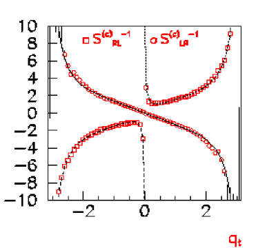
Figure 1:

Components of the charged fermion propagator, $(S^{c}_{RL}(q))^{-1}$ and $(S^{c}_{LR}(q))^{-1}$. From ref. [55].

This ansatz contains a free LH charged fermion, which is what we are aiming for. (In fact, a similar ansatz describes the propagator for the neutral fermion $\psi^{n}=\Phi\psi^{c}$ (not shown, cf. ref. [55]), for which shift symmetry [59] implies a form as in eq. (36) with $P_{R}$ and $P_{L}$ interchanged and with $M(q)$ exactly the Wilson mass term, with only $h(q)$ not determined by this symmetry.) Comparing this ansatz with the figure, we find that

$$h(q)\sim\cases{1/q^{2}\,,&$q$ small\,,\cr 1\,,&$q\sim(\pi,0),(0,\pi),(\pi,\pi)$\cr}$$ (37)

(an example of such a function is $h(q)^{-1}=\sum_{\mu}\sin^{2}{p_{\mu}}+(1-\prod_{\mu}\cos^{2}{(p_{\mu}/2)})^{2}$). This pole is visible in the figure in the data for $(S^{c}_{RL}(q))^{-1}$. This implies that the RH part of the inverse charged propagator is singular near $q=0$, the necessary condition for avoiding the Nielsen–Ninomiya theorem. However, this singularity, if our ansatz is correct, represents a pole in the inverse propagator. Through the Ward identities for the symmetry (28) (with $h_{L}$ constant), this implies the existence of a pole in the vertex function, because the charged RH channel couples to the gauge field. Such poles may in general lead to unphysical contributions to the $\beta$-function of the full theory [6, 7].

I believe that the puzzle about the nature of this singularity which apparently is present in the data should be resolved in order to assess the viability of this approach to putting ChGTs on the lattice. While it does look that the model reviewed here contains an undoubled LH charged fermion, it is not clear that there are no other light or massless unphysical modes. It should be noted that it is quite possible that the behavior sketched here is specific to two dimensions. An analytic study, or a more detailed numerical study, if feasible, would obviously be helpful in interpreting the data appropriately. I will return to this approach toward the end of this section.

3.2 Gauge fixing method

An alternative gauge non-invariant approach keeps the fermions and the gauge fields on the same lattice, but employs gauge fixing in order to control the gdofs [60, 61, 62, 63]. The central observation is that gauge fixing gives us the possibility to control both the transverse and longitudinal gauge fields in lattice perturbation theory, provided a suitable lattice action is chosen [61] (see below). In particular, gauge fixing suppresses fluctuations of the longitudinal components (the gdofs), and we will see that this makes it possible to keep the fermions chiral, unlike e.g. the example discussed in the Introduction. However, as we will see, in order to turn lattice perturbation theory into a valid, systematic expansion scheme, non-perturbative considerations are important.

Again, I will consider Wilson fermions, with a momentum-dependent mass term as in eq. (1) in order to remove doublers. In the gauge-fixing approach one adds to the naively discretized theory with charged LH fermions and neutral RH fermions the terms

$$-\frac{r}{2}({\overline{\psi}}^{n}_{R}\kern 0.5pt{\lower 0.1pt\vbox{\hrule height=0.5pt,width=6.8pt\hbox{\vrule width=0.5pt,height=6.0pt\kern 6.0pt\vrule width=0.3pt} \hrule height=0.3pt,width=6.8pt}}\kern 1.5pt\psi^{c}_{L}+{\rm h.c.})+{\tilde{\kappa}}(\partial_{\mu}A_{\mu})^{2}$$ (38)

$$+\kappa A_{\mu}^{2}+{\rm other\ counter\ terms}+{\rm ghosts}\,,$$

$${\tilde{\kappa}}=\frac{1}{2\xi g^{2}}\,,$$

where $\xi$ is the gauge parameter, and $\kappa A_{\mu}^{2}$ is a mass counter term. Note that the parameter ${\tilde{\kappa}}$ controls the longitudinal fluctuations just like $\beta=1/g^{2}$ controls the transverse fluctuations. Because the Wilson mass term breaks gauge invariance, there is no BRST invariance on the lattice, and counter terms will be needed in order to recover the Slavnov–Taylor identities in the continuum limit [60]. I will limit myself to the abelian case, for which no ghost fields are needed [64]. Addition of the covariant gauge-fixing term in eq. (38) makes the theory perturbatively renormalizable, and this determines the form of the counter terms: one simply has to add all possible terms up to mass dimension 4 consistent with the exact symmetries of the regulated theory. The most important of these is the gauge-field mass term; all others are of dimension 4 (because of shift symmetries [59, 60]). To this point, we are just describing what happens if one uses a gauge non-invariant perturbative regulator.

Of course, for this to work non-perturbatively, the lattice version of the gauge-fixing term proportional to $(\partial_{\mu}A_{\mu})^{2}$ has to be chosen such that the (non-perturbative) phase diagram of the lattice theory has a critical point which is described by this perturbative expansion. One has to choose the lattice gauge-fixing action such that the perturbative vacuum $A=0$ (or, on the lattice, $U=1$) gives the dominant contribution in a saddle-point approximation to the lattice theory. That this can be done was shown in ref. [62]. The idea is to choose a gauge-fixing term on the lattice roughly of the form ${\tilde{\kappa}}[(\partial\cdot A)^{2}+A^{6}]$, with the irrelevant $A^{6}$ term stabilizing the perturbative vacuum $A=0$, without otherwise affecting the long-distance behavior. (This shape can be maintained to all orders in perturbation theory by adjusting the counter terms.) The phase diagram which emerges is shown in fig. 2, where only the $\kappa$-${\tilde{\kappa}}$ plane is shown [61, 62, 65, 66] (see these refs. for other counter terms).

Consider first the theory without fermions. In a bounded region around the origin, i.e. for small $\kappa$ and ${\tilde{\kappa}}$, the gauge-fixing and mass terms do not change the critical behavior of the theory: this region of the phase diagram is filled by a Coulomb phase [51]. Since ${\tilde{\kappa}}$ is small, WCPT does not apply in this region. For large ${\tilde{\kappa}}$, WCPT is applicable, and one finds a critical line where the gauge field is massless by tuning the counter term $\kappa$ to a critical value $\kappa_{c}({\tilde{\kappa}})$. For $\kappa$ too large, $m^{2}_{A}\propto\kappa-\kappa_{c}$ is positive, and the gauge field acquires a mass. For $\kappa$ too small, $m^{2}_{A}<0$, which signals symmetry breaking. Since in this case $A_{\mu}$ acquires an expectation value $\langle A_{\mu}\rangle\neq 0$, the broken symmetry is hypercubic invariance!

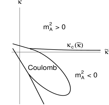
Figure 2:

Sketch of the relevant part of the phase diagram for the gauge-fixing approach. For full details on the complete diagram, see ref. [66].

Moreover, with our choice of irrelevant terms ($A^{6}$), this transition is continuous. To lowest order in WCPT, the classical potential for the gauge field is (roughly)

$$V_{\rm cl}=\kappa A^{2}+{\tilde{\kappa}}A^{6}\,.$$ (39)

Without the $A^{6}$ term, we would find a first order phase transition going from $\kappa>\kappa_{c}$ to $\kappa<\kappa_{c}$ (where at tree level $\kappa_{c}=0$), but with the $A^{6}$ term, the transition is continuous. We see that the usual adjustment of the gauge-field mass counter term corresponds, as desired, to a continuous phase transition between two distinct phases above and below the critical line $\kappa=\kappa_{c}({\tilde{\kappa}})$. For details, see refs. [66, 65] (for an earlier informal account, see ref. [67]). A naive discretization of $(\partial\cdot A)^{2}$ without the $A^{6}$-like term leads to a very different phase diagram, without the desired critical behavior [61, 66].

We thus recover Maxwell theory (without fermions, thus far) in two different ways: inside the Coulomb phase, and for large ${\tilde{\kappa}}$ near the critical line $\kappa=\kappa_{c}({\tilde{\kappa}})$. The difference is that lattice perturbation theory only applies in the latter case, and this will be essential to our goal of obtaining undoubled chiral fermions. Inside the Coulomb phase, the situation would be similar to the example in the Introduction; the gauge-fixing term would not be strong enough to control the longitudinal gauge field, i.e. the gdofs.

We now turn to the fermions. First, since they are coupled to the gauge field through the gauge coupling $g$, which is small, one expects no qualitative change in the nature of the phase diagram. The issue is whether the “back reaction” of the gauge fields, in particular the gdofs, is small as well. Since this is now also governed by WCPT, one expects that the fermion spectrum does not differ from that of the classical continuum limit. This is precisely what we find. Because the danger resides in the dynamics of the gdofs, it is enough to consider (again, as we did in the two-cutoff approach) only the interactions between the fermions and the gdofs. As in eq. (2), we rotate $\psi^{c}_{L}\to e^{i\lambda}\psi^{c}_{L}$, and we set $A_{\mu}=\partial_{\mu}\lambda$, under which eq. (38) goes over into

$$-\frac{r}{2}({\overline{\psi}}^{n}_{R}\kern 0.5pt{\lower 0.1pt\vbox{\hrule height=0.5pt,width=6.8pt\hbox{\vrule width=0.5pt,height=6.0pt\kern 6.0pt\vrule width=0.3pt} \hrule height=0.3pt,width=6.8pt}}\kern 1.5pt(e^{i\lambda}\psi^{c}_{L})+{\rm h.c.})$$ (40)

$$+{\tilde{\kappa}}(\kern 0.5pt{\lower 0.1pt\vbox{\hrule height=0.5pt,width=6.8pt\hbox{\vrule width=0.5pt,height=6.0pt\kern 6.0pt\vrule width=0.3pt} \hrule height=0.3pt,width=6.8pt}}\kern 1.5pt\lambda)^{2}+\kappa(\partial_{\mu}\lambda)^{2}+\dots\,,$$

where $\dots$ stand for the various $\lambda$ self interactions coming from the lattice versions of the gauge-fixing, mass, and other counter terms. This model can be studied in WCPT in $1/\sqrt{{\tilde{\kappa}}}$ by rescaling $\lambda=\theta/\sqrt{2{\tilde{\kappa}}}$ [61, 68]. The following heuristic arguments describe what happens.

First, near $\kappa=\kappa_{c}$ the $\theta$ propagator goes like $1/p^{4}$, i.e. the $\theta$ field has mass dimension zero. Moreover, one finds that [68]

$$\langle\Phi\rangle = \langle e^{i\lambda}\rangle\sim(\kappa-\kappa_{c})^{\eta}\,,$$ (41)

$$\eta = \frac{1}{32\pi^{2}{\tilde{\kappa}}}\,.$$

This is analogous to the behavior of a near massless scalar in two dimensions [69]. This means that at $\kappa=\kappa_{c}$ the LH and RH symmetries ($h_{L}$ and $h_{R}$ in eq. (28)) are unbroken. This is an important result: we are after a ChGT with unbroken gauge symmetry, wherein the gdofs $\Phi$ are to decouple completely!

Second, we may now expand the Wilson term in eq. (40), obtaining

$$-\frac{r}{2}{\overline{\psi}}^{n}_{R}\kern 0.5pt{\lower 0.1pt\vbox{\hrule height=0.5pt,width=6.8pt\hbox{\vrule width=0.5pt,height=6.0pt\kern 6.0pt\vrule width=0.3pt} \hrule height=0.3pt,width=6.8pt}}\kern 1.5pt\psi^{c}_{L}-i\frac{r}{2}\frac{1}{\sqrt{2{\tilde{\kappa}}}}{\overline{\psi}}^{n}_{R}\kern 0.5pt{\lower 0.1pt\vbox{\hrule height=0.5pt,width=6.8pt\hbox{\vrule width=0.5pt,height=6.0pt\kern 6.0pt\vrule width=0.3pt} \hrule height=0.3pt,width=6.8pt}}\kern 1.5pt(\theta\psi^{c}_{L})+O(\frac{1}{{\tilde{\kappa}}})+{\rm h.c.}$$ (42)

The first term is the standard Wilson term, removing the fermion doublers. In addition, we see that the interaction terms between the fermions and the field $\theta$ are all of dimension 5, and hence irrelevant! They may lead to contact terms in fermionic correlation functions, but they do not change the long-distance behavior of the fermion fields.

Of course, a more rigorous argument is needed to confirm this picture in the presence of the unusual infrared singular behavior of the $\theta$ field. A study in one-loop resummed WCPT was performed in ref. [68], and detailed (quenched) numerical computations were done in ref. [70, 65]. The numerical and analytic calculations are in good quantitative agreement with each other, and confirm the analysis described above. We conclude that this theory contains undoubled chiral fermions, with the LH charged fermion coupling to the gauge field, and the RH neutral fermion decoupling in the continuum limit. The gdofs ($\theta$) decouple in the continuum limit as well, as they should. The gauge-fixing action gives the gdofs the sophisticated dynamics alluded to in the Introduction. Since the transverse gauge field couples weakly to the fermions, one does not expect any drastic change from our conclusions in the full theory containing both dynamical fermions and the full gauge field.

The central idea in this approach is to secure renormalizability even in the absence of gauge invariance. The key ingredient is gauge fixing, and one would therefore expect universality with respect to the choice of lattice fermions. This was indeed confirmed by a combined perturbative and numerical study using domain-wall fermions instead of Wilson fermions [71].

The main issue in extending this method to non-abelian ChGTs is the existence of Gribov copies. Little work has been done in this direction at present, and therefore I will not devote much space to it here. A promising approach appears to be to use the non-perturbative gauge-fixing method proposed by Jona-Lasinio and Parrinello and by Zwanziger [72]. For speculative thoughts on how to apply this method to ChGTs, see ref. [73].

3.3 Comparison between gauge-fixing and two-cutoff methods

As in subsection 3.1, we may again ask what happens to the charged fermion propagator in the gauge-fixing approach. The charged RH fermion field is, as before,

$$\psi^{c}_{R}=\Phi^{\dagger}\psi^{n}_{R}=e^{-i\theta/\sqrt{2{\tilde{\kappa}}}}\psi^{n}_{R}\,,$$ (43)

but now with $\theta$ describing the modes of the scalar field $\Phi$. Since this scalar field decouples from the fermions for $a\to 0$, this composite operator describes exactly what it shows: a multiparticle state composed of RH neutral fermions and (higher-derivative) scalars in the continuum limit. The LH charged fermion itself is a free field in the model of eq. (40), and one finds for the LH, resp. RH components of the charged fermion propagator [68, 67]

$$P_{L}S^{c}(p)P_{R}\sim P_{L}\frac{1}{p\!\!\!/}\,,\ P_{R}S^{c}(p)P_{L}\sim P_{R}\frac{1}{p\!\!\!/}\,p^{4\eta}\,,$$ (44)

with $\eta$ given in eq. (41). We see that, also in the gauge-fixing approach, the inverse charged propagator does not have a continuous derivative at $p=0$. But now this singularity takes the form of a cut occurring in the RH channel, as one would expect if $\psi^{c}_{R}$ creates a multiparticle state. Because all these excitations ($\psi^{n}_{R}$ and $\theta$) are massless, the cut has a branch point at $p=0$.

It is interesting to compare this with our interpretation of what happens in the two-cutoff approach. In both approaches the unphysical scalars decouple, but in different ways. In the two-cutoff study, the gdofs get a mass of order the cutoff $1/b$, while in the gauge-fixing case, they are massless at the relevant critical point, but have no interactions with the physical sector. One would expect that these two different ways of decoupling the gdofs lead to different singularities in the charged fermion propagator. It is possible that the pole-like singularity exhibited in fig. 1 is a finite-volume artifact, and would turn into a branch point in infinite volume. However, the existence of a branch point at $p=0$ is difficult to reconcile with scalar fields with a mass of order the cutoff. Clearly, a better understanding is needed for the two-cutoff method.

4 Conclusion

In this talk, I have covered what I consider the most important developments since the last general review of this field [26]. There has been a tremendous amount of progress, and we appear to be much closer to satisfactory constructions of lattice ChGTs. However, the job is not done yet.

Around the time of Shamir’s 1995 review, the fundamental problem with regard to maintaining the chiral fermion spectrum in the presence of interactions with gdofs had been well understood, and both the gauge-fixing and the two-cutoff or interpolation methods have been proposed in order to specifically address this issue.

More recently, Lüscher has realized that it may even be possible to formulate ChGTs on the lattice in a manifestly gauge-invariant way, provided that (at least) the fermion representation is anomaly free. In this approach, the Nielsen–Ninomiya theorem is circumvented by modifying chiral symmetry on the lattice such that it yields the usual chiral Ward identities in the continuum limit, and yet does not lead to species doubling. In order to define ChGTs, the phase of the chiral determinant has to be chosen so as to not violate gauge invariance. Obviously, the advantage of a manifestly gauge-invariant construction is that the gdofs decouple already from the physical excitations at finite lattice spacing.

In order to show that ChGTs can be put on the lattice in a gauge-invariant way, a complete classification of all anomalies, both local and global, is necessary. Such a classification was accomplished for the case of abelian ChGTs. A crucial element is the admissibility constraint eq. (26). It is interesting to observe that, while this constraint is not expected to change the universality class in the weak-coupling limit [15], it does change the strong-coupling behavior of this lattice version of ChGTs relative to that of vector-like theories. For the non-abelian case, there is a conjecture that the standard anomaly-cancellation condition $d^{abc}=0$ is sufficient for removing all local anomalies. Little is known at present about a classification of global obstructions and their possible dependence on boundary conditions.

It is interesting to compare this state of affairs with the gauge-fixing approach. The latter approach also has succeeded in formulating abelian ChGTs on the lattice, while it is presently unknown whether it can be extended to the non-abelian case. Both methods admit weak-coupling perturbation theory, and both are perturbatively renormalizable. In both cases unitarity is not manifest, but could in principle be established perturbatively to all orders.

Of course, in principle, there is a theoretical advantage in having a manifestly gauge-invariant formulation on the lattice. However, even in the abelian case, where progress has been sufficient to compare the two methods, this advantage comes at a price. It is clear that the gauge-invariant approach is more difficult to implement numerically, because it is numerically very expensive to compute the overlap-Dirac operator, or equivalently, ${\hat{\gamma}}_{5}$. Other approaches, such as gauge fixing, may be technically simpler, even if they lack exact gauge invariance at the regularized level. It is important to remember that what is required is only the recovery of gauge invariance in the continuum limit, i.e. at scales much below the cutoff $1/a$. An assumption here is, of course, that the various different ways of putting ChGTs on the lattice all describe the same universality class.

At present, there exists two types of gauge non-invariant methods, the one based on gauge fixing discussed above, and the two-cutoff or interpolation approach. The way in which the gauge-fixing methods avoids the Nielsen–Ninomiya theorem is well understood, and it has been demonstrated both analytically and numerically that chiral fermions can be put on the lattice. The main problem lies in the extension of this approach to non-abelian ChGTs, because of the issue of Gribov copies. This cannot be said of the two-cutoff approach, in which the behavior of the fermion spectrum is not fully understood beyond perturbation theory. The work of ref. [55] has contributed significantly to a clarification of what the important open problems are in this respect. I believe that it is important to gain more analytic insight in this case in order to assess its viability.

An issue which I did not touch on in this review is that of fermion-number violation. In my view, this issue is not central to the problem of constructing lattice ChGTs. If an approach is successful, this particular problem “will take care of itself.” This does not imply that it is not interesting to understand in detail how this works out for a given approach. For general discussions of the problem within the context of lattice ChGTs, see refs. [74, 75, 76]. In the gauge invariant approach, fermion number is violated just as it is in the continuum, through the measure of the fermionic path integral [15]. For the two-cutoff approach, see refs. [46, 47], and for the gauge-fixing approach, see ref. [68].

Finally, there is the question whether it will ever be possible to investigate ChGTs dynamically on the lattice. After all, while it is interesting to learn how ChGTs may be put on the lattice, one would like to learn more about issues such as dynamical symmetry breaking in ChGTs, for which also analytic methods have contributed relatively little insight. While full-fledged numerical simulations are clearly not within reach yet (the hardest problem being that of a complex measure [77]), it may be possible to probe, within a given approach, the phase of the fermion determinant, for instance on an ensemble of quenched configurations. The behavior of the fluctuations of the phase of the determinant should tell us something about how different ChGTs are dynamically from vector-like gauge theories. Of course, we are not there yet, since non-abelian ChGTs are more interesting than abelian ChGTs, and the task of putting non-abelian ChGTs on the lattice has not yet been completed.

Acknowledgements

I thank the organizers of Lattice 2000 for giving me the opportunity to present this review. I also thank Oliver Bär, Subhasis Basak, Geoff Bodwin, Michael Creutz, Asit De, Robert Edwards, Pilar Hernández, Jiří Jersák, Yoshio Kikukawa, Martin Lüscher, Jun Nishimura, Michael Ogilvie, Noam Shoresh, Hiroshi Suzuki, and, in particular Yigal Shamir and Steve Sharpe, for discussions and comments, as well as the INT at the Univ. of Washington for hospitality. This work is supported in part by the US Dept. of Energy.

References

- [1] L. Karsten, J. Smit, Nucl. Phys. B183 (1981) 103
- [2] H. Nielsen, M. Ninomiya, Nucl. Phys. B185 (1981) 20 (Erratum: B195 (1982) 541); Nucl. Phys. B193 (1981) 173
- [3] S. Drell, M. Weinstein, S. Yankielowicz, Phys. Rev. D14 (1976):1627; H. Quinn, M. Weinstein, Phys. Rev. Lett. 57 (1986) 2617
- [4] C. Rebbi, Phys. Lett. B186 (1987) 200
- [5] L. Karsten, J. Smit, Nucl. Phys. B144 (1978) 536; Phys. Lett. B85 (1979) 100
- [6] G. Bodwin, E. Kovacs, Phys. Lett. B193 (1987) 283; Phys. Rev. D37 (1988) 1008
- [7] A. Pelissetto, Ann. Phys. 182 (1988) 177
- [8] K. Wilson, Phys. Rev. D10 (1974) 2445
- [9] D. Petcher, Nucl. Phys. B (Proc. Suppl.) 30 (1993) 50 and refs. therein
- [10] I. Montvay, Phys. Lett. B199 (1987) 89
- [11] M. Lüscher, Phys. Lett. B428 (1998) 342
- [12] P. Ginsparg, K. Wilson, Phys. Rev. D25 (1982) 2649
- [13] H. Neuberger, Phys. Lett. B417 (1998) 141; Phys. Lett. B427 (1998) 353
- [14] M. Creutz, hep-lat/0007032
- [15] M. Lüscher, Nucl. Phys. B549 (1999) 295
- [16] F. Niedermayer, Nucl. Phys. B (Proc. Suppl.) 73 (1999) 105
- [17] R. Narayanan, Phys. Rev. D58 (1998) 097501
- [18] Y. Kikukawa, A. Yamada, hep-lat/9810024
- [19] R. Narayanan, H. Neuberger, Phys. Rev. Lett. 71 (1993) 3251; Nucl. Phys. B443 (1995) 305
- [20] P. Hernández, K. Jansen, M. Lüscher, Nucl. Phys. B552 (1999) 363
- [21] R. Narayanan, H. Neuberger, Nucl. Phys. B477 (1996) 521
- [22] T. Izubuchi, J. Nishimura, JHEP 9910 (1999) 002; Nucl. Phys. B (Proc. Suppl.) 73 (1999) 691
- [23] M. Golterman, Y. Shamir, Phys. Lett. B353 (1995) 84 (Erratum: B359 (1995) 422)
- [24] M. Lüscher, Nucl. Phys. B568 (2000) 162; see also M. Lüscher, Nucl. Phys. B (Proc. Suppl.) 83 (2000) 34
- [25] T. Fujiwara, H. Suzuki, K. Wu, Phys. Lett. B463 (1999) 63; Nucl. Phys. B569 (2000) 643
- [26] Y. Shamir, Nucl. Phys. B (Proc. Suppl.) 47 (1996) 212
- [27] R. Stora, in Progress in Gauge Field Theory (Cargèse 1983), eds. G. ’t Hooft et al. (Plenum, 1984); B. Zumino, in Relativity, Groups and Topology (Les Houches 1984), eds. B. deWitt, R. Stora (North-Holland, 1984)
- [28] M. Lüscher, Nucl. Phys. B538 (1999) 515
- [29] H. Neuberger, hep-lat/0002032
- [30] M. Lüscher, JHEP 0006 (2000) 028
- [31] H. Suzuki, Nucl. Phys. B585 (2000) 471
- [32] J. Wess, B. Zumino, Phys. Lett. B37 (1971) 95
- [33] D. Kaplan, Phys. Lett. B288 (1992) 342
- [34] Y. Shamir, Nucl. Phys. B406 (1993) 90; V. Furman, Y. Shamir, Nucl. Phys. B439 (1995) 54
- [35] P. Vranas, these proceedings.
- [36] T. Aoyama, Y. Kikukawa, hep-lat/9905003
- [37] L. Alvarez-Gaume, S. Della Pietra, V. Della Pietra, Phys. Lett. B166 (1986) 177; Comm. Math. Phys. 109 (1987) 691
- [38] D. Kaplan, M. Schmaltz, Phys. Lett. B368 (1996) 44
- [39] Y. Kikukawa, Y. Nakayama, hep-lat/0005015
- [40] O. Bär, I. Campos, Nucl. Phys. B581 (2000) 499
- [41] E. Witten, Phys. Lett. B117 (1982) 324
- [42] D. Adams, hep-lat/9910036; Nucl. Phys. B589 (2000) 633
- [43] Y. Shamir, Phys. Rev. Lett. 71 (1993) 2691; hep-lat/9307002
- [44] M. Göckeler et al., Nucl. Phys. B404 (1993) 839
- [45] G. ’t Hooft, Phys. Lett. B349 (1995) 491
- [46] P. Hernández, R. Sundrum, Nucl. Phys. B455 (1995) 287
- [47] G. Bodwin, Phys. Rev. D54 (1996) 6497
- [48] S. Hsu, hep-th/9503058
- [49] A. Slavnov, Nucl. Phys. B (Proc. Suppl.) 42 (1995) 166
- [50] V. Bornyakov et al., in Lattice Fermions and the Structure of the Vacuum, eds. V. Mitrjushkin, G. Schierholz (Kluwer, 2000) (hep-lat/0003001)
- [51] D. Foerster, H. Nielsen, M. Ninomiya, Phys. Lett. B94 (1980) 135
- [52] E. Fradkin, S. Shenker, Phys. Rev. D19 (1979) 3682
- [53] P. Hernández, R. Sundrum, Nucl. Phys. B472 (1996) 334
- [54] G. Bodwin, Nucl. Phys. B (Proc. Suppl.) 53 (1997) 644
- [55] P. Hernández, P. Boucaud, Nucl. Phys. B513 (1998) 593
- [56] G. Schierholz, these proceedings
- [57] E. Eichten, J. Preskill, Nucl. Phys. B268 (1986) 179
- [58] M. Golterman, D. Petcher, E. Rivas, Nucl. Phys. B395 (1993) 596
- [59] M. Golterman, D. Petcher, Phys. Lett. B225 (1989) 159
- [60] A. Borrelli et al., Nucl. Phys. B333 (1990) 335
- [61] Y. Shamir, Phys. Rev. D57 (1998) 132
- [62] M. Golterman, Y. Shamir, Phys. Lett. B399 (1997) 148
- [63] J. Vink, Phys. Lett. B321 (1994) 239
- [64] W. Bock, M. Golterman, Y. Shamir, Phys. Rev. D58 (1998) 097504
- [65] W. Bock, M. Golterman, Y. Shamir, Phys. Rev. D58 (1998) 054506
- [66] W. Bock et al., Phys. Rev. D62 (2000) 034507
- [67] W. Bock, M. Golterman, Y. Shamir, Nucl. Phys. B (Proc. Suppl.) 63 (1998) 147; 581
- [68] W. Bock, M. Golterman, Y. Shamir, Phys. Rev. D58 (1998) 034501
- [69] S. Coleman, Comm. Math. Phys. 31 (1973) 259; N. Mermin, H. Wagner, Phys. Rev. Lett. 17 (1966) 1133
- [70] W. Bock, M. Golterman, Y. Shamir, Phys. Rev. Lett. 80 (1998) 3444
- [71] S. Basak, A. De, hep-lat/9911029; these proceedings (hep-lat/0011018)
- [72] C. Parrinello, G. Jona-Lasinio, Phys. Lett. B251 (1990) 175; D. Zwanziger, Nucl. Phys. B345 (1990) 461
- [73] W. Bock et al., in Lattice Fermions and the Structure of the Vacuum, eds. V. Mitrjushkin, G. Schierholz (Kluwer, 2000) (hep-lat/9912025)
- [74] T. Banks, Phys. Lett. B272 (1991) 75; T. Banks, A. Dabholkar, Phys. Rev. D46 (1992) 4016
- [75] M. Dugan, A. Manohar, Phys. Lett. B265 (1991) 137
- [76] W. Bock, J. Hetrick, J. Smit, Nucl. Phys. B437 (1995) 585
- [77] S. Chandrasekharan, these proceedings (hep-lat/0011022)