QCD at a Finite Density of Static Quarks

Abstract

Recently, cluster methods have been used to solve a variety of sign problems including those that arise in the presence of fermions. In all cases an analytic partial re-summation over a class of configurations in the path integral was necessary. Here the new ideas are illustrated using the example of QCD at a finite density of static quarks. In this limit the sign problem simplifies since the fermionic part decouples. Furthermore, the problem can be solved completely when the gauge dynamics is replaced by a Potts model. On the other hand in QCD with light quarks the solution will require a partial re-summation over both fermionic and gauge degrees of freedom. The new approach points to unexplored directions in the search for a solution to this more challenging sign problem.

1 INTRODUCTION

Although lattice field theories allow for a completely non-perturbative definition of a quantum field theory, computational limitations impose severe restrictions on our ability to perform calculations in them. At the beginning of the new millennium many important questions that arise in a variety of fields like strongly interacting fermionic systems, frustrated systems, systems with $\theta$-vacuum, chiral gauge theories and real time dynamics in quantum field theories, remain unanswered. A common problem that hinders progress in all these areas is the “sign problem”, which arises due to the inability to isolate the appropriate probabilistic measure for a stochastic computation.

One is typically interested in the partition function of a quantum many body system which can be compactly written as

$$Z\;=\;{\rm Tr}\left[\exp(-H/T)\right]\;=\;\sum_{[C]}W[C]$$ (1)

where the sum over configurations $C$ is used to evaluate the trace through the Feynman path integral in a convenient basis. In general $W[C]$, the Boltzmann weight of the configuration, is not guaranteed to be positive definite. The difficulty in finding the right class of configurations such that $W(C)$ is positive definite is referred to as the sign problem. However, since $Z$ itself is positive definite a summation over a sufficiently large number of configurations should always yield a positive answer. Unfortunately, the number of configurations required grows exponentially with the volume; it is hopeless to require even a computer to perform the re-summation.

Recently, a lot of progress has been made in solving sign problems using cluster methods since it is sometimes possible to analytically sum over all the configurations that are obtained through cluster flips. Furthermore, this class of configurations can grow exponentially with volume. Interestingly, every known type of cluster algorithm has been applied to solve to a new type of sign problem. The first solution was found in a classical $O(3)$ model with a $\theta$ parameter which makes the action complex [1]. It was shown that a summation over flips of Wolff clusters [2] produced only positive (or zero) weights. More recently, it was discovered that in certain four-Fermi models a similar result emerges when one uses loop clusters known from quantum spin systems [3]. This has been used to eliminate sign problems that arise due to Fermi statistics [4, 5]. Sign problems in Potts models due to a complex action can be solved using clusters of the Swendsen-Wang algorithm[6].

In this article the above progress is reviewed using the example of the Potts model which relevant to QCD at a finite density of static quarks. The next section contains a review of the sign problem in QCD with a new perspective on its “physical origin”. It is argued that the sign problem has two parts, one coming from Gauss law type constraints and the other from fermion permutations. The later sections show that the recent progress has produced examples in which both types of sign problems can be solved separately. In simple cases it may be possible to find solutions to the combined problem in the near future.

2 THE SIGN PROBLEM IN QCD

The partition function in QCD is usually written as a path integral over fermionic and gauge fields. Instead of representing fermions as Grassmann variables, for computational reasons they are integrated out in favor of a fermion determinant. The final result takes the form

$$Z_{\rm QCD}\;=\;\int\;[dU]\;\exp\left(-S_{G}[U]\right)\;{\rm Det}(D[U])$$ (2)

where $D$ is the Dirac operator. Given that the gauge field action $S_{G}[U]$ is real the usual claim is that sign problems arise from the fermion determinant. As is well known in the presence of a chemical potential the fermion determinant ${\rm Det}(D[U])$ becomes complex. Although this description is quite accurate, it is a bit unsatisfactory since a lot of interesting dynamics of quarks has been pushed into the calculation of the fermion determinant. Exposing the anatomy of the fermion determinant may reveal some deeper “physical origin” to the sign problem. This can be illustrated by a simple example.

Consider compact QED instead of QCD. The partition function in that case is similar to (2) except that the integration is over $U(1)$ gauge fields instead of $SU(3)$. Again adding a chemical potential makes the fermion determinant complex and hence introduces a sign problem for the same reasons as in QCD. But in this case it is possible to understand the origin of the sign problem at a more deeper level. If the fermion determinant is expanded as a sum over electron and positron world line configurations, the configurations that dominate at non-zero chemical potentials would contain more electrons than positrons. However, due to Gauss’s law it is impossible to have more electrons than positrons in a periodic box. Hence, the weight of such configurations must be zero once Gauss’s law is imposed. Since it is the integral over the gauge fields that enforces Gauss’s law, it is natural to have both positive and negative contributions in the path integral for a fixed gauge field configuration. The negative signs can help cancel the wrong configurations. Understanding the “physical” origin of the sign problem makes the solution clear. In the case of QED, one must throw away all fermionic configurations in which there are more electrons than positrons. This effectively means the chemical potential has no effect on the partition function which is a well known fact [7].

Unfortunately, fermionic world line configurations have sign problems of their own that arise from the Pauli principle. When fermions travel in imaginary time their positions can get permuted. Whenever this permutation is odd the configuration weight is negative. Thus, performing the integration over the gauge field configurations alone in general will not yield a positive weight for a fermionic configuration. In fact the sign problem in QCD arises due to an intricate mixture of fermion permutation sign and a more difficult constraints one of which is the Gauss’s law. The example from QED suggests that it may be useful to consider a regrouping of both fermion and gauge field configurations in the search to find positive definite weights.

3 THE STATIC QUARK LIMIT

There are special limits where the sign problem becomes much simpler. One is the limit of static quarks. Here the fermions cannot permute with each other and so problems arise only from Gauss’s law type constraints. This simplification has prompted a variety of research on the physics of QCD with a finite density of static quarks. However, adding chemical potential to quarks that are infinitely massive is a bit subtle. In order to induce a finite density of static quarks one needs to take the chemical potential to infinity along with the quark mass always keeping the chemical potential larger than the rest mass of the quarks. This limit was originally formulated in [7] and later studied in [8]. More recently the partition function for a fixed baryon number in the static quark limit was studied in [9]. An equivalent but simpler approach to the limit of static quarks can be formulated by recognizing that the partition function for $n$ quarks and $\bar{n}$ antiquarks of mass $m$ in the static limit is given by

$$Z_{n,\bar{n}}\;=\;\int\;[dU]\;\frac{\Phi^{n}}{n!}\;\frac{{\Phi^{*}}^{\bar{n}}}{\bar{n}!}\;{\rm e}^{-S_{G}[U]-m(n+\bar{n})N_{t}}$$ (3)

where $S_{G}[U]$ is the gauge action on a $N_{s}^{3}N_{t}$ lattice. The gauge coupling $\beta$ is implicit in the definition of $S_{G}$. The quantity $\Phi$ is the sum over the trace of Polyakov lines at every spatial point ${\mathbf{x}}$,

$$\Phi=\sum_{\mathbf{x}}Tr\left(\prod_{t=0}^{N_{t}-1}U_{0}({\mathbf{x}},t)\right),$$ (4)

with $U_{0}({\mathbf{x}},t)$ representing the time like links. The grand canonical partition function is then given by

$$Z = \sum_{n,\bar{n}}Z_{n,\bar{n}}\exp\left(\mu(n-\bar{n})/T\right)$$ (5)

$$= \int\;[dU]\;{\rm e}^{-S_{G}[U]+h\;\Phi+h^{\prime}\;\Phi^{*}}$$ (6)

where $h={\rm e}^{-(m-\mu)N_{t}}$ and $h^{\prime}={\rm e}^{-(m+\mu)N_{t}}$. The static quark limit is obtained by taking the $m\rightarrow\infty$ and $\mu\rightarrow\infty$ limits with $h={\rm e}^{-(m-\mu)N_{t}}$ fixed. In this limit $h^{\prime}\rightarrow 0$. Note that although the above approach treats quarks as bosons instead of fermions, at finite densities in the continuum limit it is impossible to distinguish between them.

Due to the complex nature of ${\rm e}^{h\Phi}$ the partition function of eq. (6) suffers from a sign problem albeit a much simpler one as compared to eq. (2). Absorbing the magnitude of this term in the Boltzmann weight, one can define the average of the phase as,

$$\langle{\rm Phase}\rangle\;=\;\frac{\int\;[dU]\;{\rm e}^{-S_{G}[U]+h{\rm Re}\Phi}\;{\rm e}^{ih{\rm Im}\Phi}}{\int\;[dU]\;{\rm e}^{-S_{G}[U]+h{\rm Re}\Phi}}.$$ (7)

Since $\langle{\rm Phase}\rangle$ is a ratio of two partition functions, in the large volume limit it will vanish exponentially. In order to make progress without solving the sign problem it is necessary to remain in volumes where the average sign is not too small. This usually puts severe restrictions on our ability to address interesting questions regarding the phase transition.

Figure 1: The phase diagram of static QCD. The point $C$ is expected to be in the universality class of the 3-d Ising model.

The phase diagram in the $\beta-h$ plane was first studied in [8]. Figure 1 shows the most likely scenario based on the well known fact that there is a first order transition on the $h=0$ line at $\beta_{c}$ due to the spontaneous breaking of the ${\mathbf{Z}_{3}}$ center symmetry. When $h\neq 0$ the symmetry is explicitly broken. However, the first order phase transition should typically persist for non-zero $h$ with decreasing latent heat ending at the second order critical point $C$ which should be governed by the 3-d Ising universality class. Although, the study in [8] could not confirm this picture it showed that the point $C$ must be quite close to the $h=0$ axis. In particular the well known discontinuity in the Polyakov line at $\beta_{c}$ disappeared at the smallest $h$ studied. This information suggests that with out solving the sign problem it may still be possible to study the behavior of the model close to the critical line of the phase diagram on lattices whose size is constrained by the closeness of the point $C$ to the $h=0$ axis.

4 SOLVING THE SIGN PROBLEM

An interesting challenge is to be able to solve the sign problem arising in eq. (6). Such a solution can perhaps teach us about solutions to other more interesting sign problems in gauge theories. In order to make progress it is useful to learn from a simpler example where the gauge dynamics is replaced with a simple 3-state Potts model. The new partition function takes the form of

$$Z=\sum_{z}{\rm e}^{\;\beta\;E[z]+hM[z]+h^{\prime}M^{*}[z]}$$ (8)

with the energy and magnetization defined by

$$E[z]=\sum_{{\mathbf{x}},i}\delta_{z_{\mathbf{x}},z_{{\mathbf{x}}+\hat{i}}},\;\;M[z]\;=\;\sum_{\mathbf{x}}z_{\mathbf{x}}.$$ (9)

Due to its symmetry properties, the three state Potts model with $z_{\mathbf{x}}\in\{1,{\rm e}^{i2\pi/3},{\rm e}^{-i2\pi/3}\}$, has been considered a useful effective model for static QCD close to the phase transition [10, 11].

An interesting solution to the sign problem in (8) was proposed in [12]. It was shown that the partition function can be rewritten in terms of new variables which describe classical statistical mechanics arising from the Hamiltonian,

$$H=\sum_{{\mathbf{x}},i}\sigma|\;l_{{\mathbf{x}},i}|\;+\sum_{\mathbf{x}}(M\;|\;n_{\mathbf{x}}|-\mu\;n_{\mathbf{x}}),$$ (10)

that represents the energy of configurations labeled by quark number distribution $n_{\mathbf{x}}\in\{-3,-2,...,3\}$ associated with sites and color flux variables $l_{{\mathbf{x}},i}\in\{-1,0,1\}$ associated with links. The configurations further obey the Gauss’s law constraint

$$\sum_{i=1}^{3}(l_{{\mathbf{x}},i}-l_{{\mathbf{x}},-i})=n_{\mathbf{x}}\;\mbox{mod}\;\;3.$$ (11)

This type of flux tube models is well known in the literature [13]. Since the Hamiltonian is real, except for the complications arising from the Gauss law constraint, the sign problem is completely solved. The introduction of new variables has helped in re-summing over classes of configurations in the original variables. In [12] a metropolis algorithm was used to study the flux tube model.

There is another way to solve the sign problem arising in (8) based on cluster algorithms for Potts models [6]. The essential idea in this case is to write the weight associated with a bond,

$${\rm e}^{\kappa\delta_{z_{x},z_{y}}}\;=\;\sum_{b=0,1}\left[\delta_{b,1}\delta_{z_{x},z_{y}}({\rm e}^{\kappa}-1)+\delta_{b,0}\right],$$ (12)

as a sum over new bond variables $b$, with $b=1$ representing the presence of a connection between the sites and $b=0$ representing the absence of a connection. Every configuration $[z,b]$ of bonds and Potts spins is made up of a connected cluster $({\cal C})$ of sites, with the property that each connected cluster of sites always contains the same Potts spin $z_{\cal C}$. This property allows the Boltzmann weight of each configuration $[z,b]$ to be written as a product over cluster weights and the partition function takes the form

$$Z=\sum_{[z,b]}\;\left\{\prod_{{\cal C}}W({\cal C})\;\exp\left(L_{\cal C}\;[hz_{\cal C}+h^{\prime}z^{*}_{\cal C}]\right)\right\},$$ (13)

where $L_{\cal C}$ represents the size of the cluster ${\cal C}$ and $W({\cal C})=({\rm e}^{\kappa}-1)^{B_{\cal C}}$ where $B_{\cal C}$ stands for the number of $b=1$ bonds in the cluster. Since $W({\cal C})$ does not depend on the spin variables, it is easy to perform a sum over the allowed cluster spin variables $z_{\cal C}\in\{1,{\rm e}^{i2\pi/3}$ and ${\rm e}^{-i2\pi/3}\}$. The partition function can finally be written as

$$Z=\sum_{[b]}\;\left\{\prod_{{\cal C}}W({\cal C})\;\left(\sum_{z}{\rm e}^{L_{\cal C}\;[hz+h^{\prime}z^{*}]}\right)\right\}.$$ (14)

It is easy to check that the Boltzmann weight in (14) for $h,h^{\prime}>0$ is always positive which solves the sign problem.

The two solutions to the sign problem sketched above suggest that an appropriate regrouping of the gauge configurations may yield a solution in the case of QCD with static quarks. However, this has not yet been achieved and remains an open problem for the future. On the other hand, based on the strong coupling expansion, a solution of the type found in the flux representation of the Potts model may be easy to find. A cluster type solution, although more exciting, could be difficult.

5 RESULTS IN THE POTTS MODEL

Recently, the partition function of eq. (8) has been studied numerically for $h=h^{\prime}$. Since in this case the action is real the model does not suffer from a sign problem. The critical region has been analyzed in great detail and the critical end point $C$ is found to be $(\beta_{c}=0.54938(2),h_{c}=0.000516(7))$ [14, 15]. The reader is referred to the original article for further results and details.

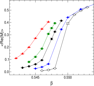
Figure 2: Expectation value of ${\rm Re}(M)$ as a function of $\beta$ for $h=0.0005$ (open circles), $0.001$ (diamonds), $0.0015$ (filled circles), $0.002$ (squares), and $0.0025$ (triangles) in the infinite volume limit.

The model with $h^{\prime}=0$ is more closer in spirit to the physics of a finite density of static quarks. Although in this case the action is complex, the sign problem can be completely solved as discussed in the previous section. Using this solution and an algorithm described in [16], the behavior of the magnetization $M$ was studied on lattices as large as $40^{3}$. Using finite size scaling analysis the were extrapolated to the infinite volume limit. In figure 2 some results are plotted as a function of $\beta$ for various values of $h$. Clearly, even for $h=0.002$ the transition has already turned into a smooth cross over. This result is quite consistent with the results of [8].

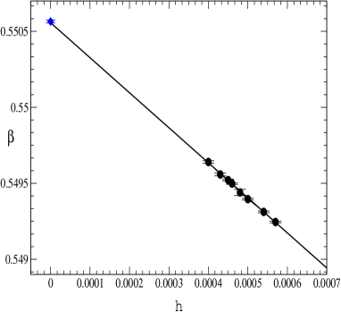
Figure 3: The critical line in the $\beta-h$ plane. The data points represent the infinite volume extrapolations of the peaks of the specific heat. The solid line is a plot of eq. (15).

Since the critical line is very close to the $h=0$ axis, the sign problem is rather mild. An estimate shows that $\langle{\rm Phase}\rangle\simeq\exp(-N_{s}^{3}/73^{3})$ suggesting that only for $N_{s}>80$ will the solution to the sign problem become necessary. In fact it appears to be more efficient to simulate the theory with the real action and absorb the complex phase into observables for smaller lattice sizes. Using this technique simulations were extended to $80^{3}$ lattices and the location of the critical line was determined using peaks in the specific heat. Figure 3, shows the data along with a fit to the critical line

$$\beta=0.550557(21)-h/0.4337(78).$$ (15)

This line extrapolates very nicely to the first order critical point on the $h=0$ axis, which is well known to be $\beta_{c}=0.550565(10)$ [17]. A preliminary analysis of the critical behavior near the end point $C$ shows consistency with the 3-d Ising model. The critical point is found to be shifted mildly to $(\beta_{c}\sim 0.5495(1),h_{c}\sim 0.000468(5))$. A more detailed discussion of the analysis will be given in [16].

6 FERMION SIGN PROBLEMS

The difficulties associated with finite density QCD are shared by much simpler four-Fermi models like the repulsive Hubbard model away from half filling. The conventional approach in interacting fermion models is to rewrite the interactions as fermion bilinears using auxiliary fields so that the fermions can be integrated out in favor of a fermion determinant, very much like in QCD. Hence it is not surprising that similar problems arise even in simple cases. An interesting question is whether one can deal with fermion interactions differently. Perhaps a more direct approach involving fermionic configurations will yield novel solutions if the fermion sign problem is tackled.

Some years ago this approach was investigated in [18]. Starting with finite density QCD in the strong coupling limit the gauge integration was performed explicitly and a purely fermionic action was obtained. The fermionic theory had six-Fermi couplings representing a baryonic mass term. Although one would naively disregard this approach as difficult, the fermionic model could be solved with a novel algorithm which used a clever partial solution to the sign problem in the model. Unfortunately, the physics of the strong coupling limit appeared rather uninteresting at high densities. It would be interesting to investigate this approach further and ask if one can extend the study beyond the leading strong coupling approximation.

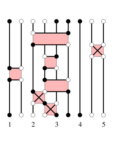
Figure 4: A typical configuration of fermion occupation numbers and clusters. The filled and open circles represent $n=1,0$. The dark lines represent connected bonds. Shaded regions represent interactions. There are five clusters in the configuration.

Over the last couple of years a new class of solutions to sign problems in a variety of four-Fermi models have emerged [4, 5]. The models are formulated directly in the fermionic Fock space, and configurations are labeled by fermion world lines. When the fermion permutation sign is taken into account with other local negative signs arising from transfer matrix elements, the partition function can be written as

$$Z=\sum_{[n]}{\rm Sign}[n]\;W[n]$$ (16)

where $[n]$ represents a fermion occupation number configuration. Since the Hilbert space of fermion occupation number states is isomorphic to that of a spin-1/2 particle, the cluster algorithms for quantum spin systems can be used to formulate algorithms for the fermions [19]. Except for subtleties arising due to Fermi statistics, this essentially means that one is able to rewrite the partition function (16) in terms of fermion occupation numbers and bonds $b$,

$$Z=\sum_{[n,b]}{\rm Sign}[n,b]\;W[n,b],$$ (17)

which is analogous to the example in the Potts model discussed in section 4. Figure 4 shows a typical fermionic configuration with an odd permutation along with clusters which have the property that by changing all the fermion occupation numbers within a cluster from 0 to 1 and vice-versa, one obtains another allowed configuration. This update is referred to as a cluster flip.

Recently, a relation between the change in the fermion permutation sign due to a cluster flip and the cluster topology was discovered [20]. The relation showed that in certain models the sum over Boltzmann weights of configurations obtained through cluster flips for a fixed set of clusters is always positive; a result strikingly similar to the example of the Potts model. This observation has been used to design an efficient fermion cluster algorithm and is referred to as the “meron cluster algorithm”. It has been applied extensively to the study of the critical behavior near a ${\mathbf{Z}}_{2}$ finite temperature chiral phase transition with staggered fermions [21, 22]. This study for the first time demonstrated the emergence of Ising critical behavior in a fermionic model confirming dimensional reduction. Figure 5 shows the chiral condensate as a function of temperature in the staggered fermion mode. The scaling form $A(T_{c}-T)^{0.314(7)}$ consistently describes the data which is with in two standard deviations of the behavior in the 3-d Ising model [22]. Dimensional reduction in fermionic models have been questioned in the past based on large $N$ calculations and results from hybrid Monte Carlo algorithms [23]. The studies using meron algorithms are beginning to convincingly show the validity of the conventional picture.

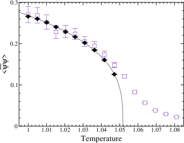
Figure 5: The critical behavior of the chiral condensate as a function of temperature in a four-Fermi model. The open squares represent results from a meron algorithm on a $32^{3}$ lattice at a mass of $m=0.001$. The black circles represent the infinite volume extrapolation. The complete results are presented in [22].

Although the number of models that can be solved with a meron cluster algorithm is limited, it continues to grow with time. Recently, new models in the family of the attractive and repulsive Hubbard models were found to be solvable. It is possible to add a chemical potential in the attractive model without violating the properties necessary for the meron algorithm to work. Such models are solvable with the hybrid Monte Carlo algorithm. However, previous studies were limited to small sizes [24]. The meron algorithm on the other hand can be implemented on much larger lattices with relative ease. Recently, this has allowed a high precision study of the Kosterlitz-Thouless transition. More details of this work can be found in [25].

7 FUTURE DIRECTIONS

The amount of progress over the last couple of years has been remarkable. A variety of physics associated with the spontaneous breaking of continuous and discrete symmetries in certain fermionic models can now be studied with high precision using a meron-cluster algorithm. Questions related to chiral perturbation theory, physics of resonances, universality classes of phase transitions, etc. which appeared difficult with hybrid Monte Carlo, can be studied much more easily. It is important to extract as much as possible from these developments.

In the context of finite density physics, there are many strongly interacting fermionic models that are still intractable. The example of QCD is a fundamental one. However, there are other models like the repulsive Hubbard model away from half filling or effective field theories of many nucleon systems, that are equally exciting to tackle. Although the solution to the problem in QCD still appears distant, the new progress suggests that solutions to the simpler theories may not be too far away. However, one should to keep in mind the difficulty of formulating cluster algorithms since the most interesting solutions to sign problems have emerged in the context of such algorithms. Limitations in cluster techniques may be correlated to our limitations in finding solutions to new sign problems.

Based on the progress made so far many new questions for the future emerge. For example:

1. Can one find a meron algorithm in a model whose ground state supports long range fermionic excitations? This can open up the possibility of studying a variety of interesting quantum phase transitions.

2. Is it possible to find an algorithm where one can update both fermionic and bosonic degrees of freedom together in an interacting model?

3. Can one extend cluster algorithms to new types of spin and gauge models? This may be possible by understanding the constraints imposed by the topology of the configuration space [26].

The answers to these questions have the potential to determine if indeed the progress of the past couple of years is just the tip of an iceberg.

Acknowledgement

I would like to thank my collaborators M. Alford, J. Cox and U.-J.Wiese for allowing me to present the preliminary results of the work on the Potts model. I would also like to thank the organizers of this conference for giving me the opportunity to present my work as a plenary talk. Finally I would like to thank the Institute for Nuclear Theory for its hospitality. Many ideas discussed here originated during the workshop on “QCD at a finite chemical potentials” organized by the INT.

References

- [1] W. Bietenholz, A. Pochinsky and U.-J. Wiese, Phys. Rev. Lett. 75, (1995) 4524.
- [2] U. Wolff, Phys. Rev. Lett. 62, (1989) 361; Nucl. Phys. B322, (1989) 759;
- [3] H.G. Evertz, G. Lana and M. Marcu, Phys. Rev. Lett. 70, (1993) 875.
- [4] S. Chandrasekharan and U.-J. Wiese, Phys. Rev. Lett. 83, (1999) 3116.
- [5] S. Chandrasekharan and U.-J. Wiese, Nucl. Phys. (Proc. Suppl.) 83-84, (1999) 774.
- [6] R. Swendsen and J.-S. Wang, Phys. Rev. Lett. 58, (1987) 86.
- [7] I. Bender, et.al., Nucl. Phys. B (Proc. Suppl.) 26, (1992) 323.
- [8] T. Blum, J.E.Hetrick and D. Toussaint, Phys. Rev. Lett 76, (1996) 1019.
- [9] J. Engels, O. Kaczmarek, F. Karsch and E. Laermann, Nucl.Phys.B558, (1999) 307-326.
- [10] L.G.Yaffe and B. Svetitsky, Phys. Rev. D26, (1982) 963.
- [11] T. A. DeGrand and C. DeTar, Nucl. Phys. B225, (1983) 590.
- [12] J. Condella and C. DeTar, Phys. Rev. D61, (2000) 074023-3.
- [13] A. Patel, Nucl Phys. B243, (1984) 411; Phys. Lett. B139, (1984) 394.
- [14] F. Karsch and S. Stickan, Phys.Lett. B488, (2000) 319.
- [15] There is a factor of 3/2 between the normalization of used here and that used in [14].
- [16] M.Alford, S.Chandrasekharan, J.Cox and U.-J.Wiese, in preparation.
- [17] W. Janke and R. Villanova, Nucl. Phys. B489, (1997) 679.
- [18] F. Karsch and K.H. Mutter, Nucl. Phys. B313, (1989) 541.
- [19] U.-J. Wiese, Phys. Lett B311, (1993) 235.
- [20] S.Chandrasekharan and J.C.Osborn, Computer Simulation Studies in Condensed Matter Physics, XIII, Eds. D.P. Landau, S.P. Lewis and H.B. Shüttler (Springer Verlag, Heidelberg, Berlin 2000).
- [21] S.Chandrasekharan, J.Cox, K. Holland and U.-J. Wiese, Nucl. Phys. B576, (2000) 481.
- [22] S. Chandrasekharan, Chinese J. of Phys. 38, (2000) 696; S.Chandrasekharan and J.C.Osborn, hep-lat/0010036.
- [23] A. Kocic and J. Kogut, Phys. Rev. Lett. 71, (1995) 3109; Nucl. Phys. B455, (1995) 229.
- [24] R. Lacaze, A. Morel, B. Petersson and J. Schröper, Eur. Phys. J. B2, (1996) 509.
- [25] J. C. Osborn, contribution to this proceedings, hep-lat/0010097.
- [26] S. Caracciolo, R. Edwards, A. Pelissetto and A. Sokal. Nucl.Phys. B403, (1993) 475.