U(1) Chiral gauge theory on lattice with gauge-fixed domain wall fermions

Abstract

We investigate a U(1) lattice chiral gauge theory ($L\chi GT$) with domain wall fermions and gauge fixing. In the reduced model limit, our perturbative and numerical investigations at Yukawa coupling $y=1$ show that there are no extra mirror chiral modes. The longitudinal gauge degrees of freedom have no effect on the free domain wall fermion spectrum consisting of opposite chiral modes at the domain wall and the anti-domain wall which have an exponentially damped overlap. Our numerical investigation at small Yukawa couplings ($y\ll 1$) also leads to similar conclusions as above.

1 Introduction

Lattice regularization of chiral gauge theories has remained a long standing problem of nonperturbative investigation of quantum field theory. Lack of chiral gauge invariance in $L\chi GT$ proposals is responsible for the longitudinal gauge degrees of freedom (dof) coupling to fermionic dof and eventually spoiling the chiral nature of the theory. The obvious remedy to control the longitudinal gauge dof is to gauge fix with a target theory in mind [1]. The formal problem is that for compact gauge-fixing a BRST-invariant partition function as well as (unnormalized) expectation values of BRST invariant operators vanish as a consequence of lattice Gribov copies [2]. Shamir and Golterman [1] have proposed to keep the gauge-fixing part of the action BRST non-invariant and tune counterterms to recover BRST in the continuum. In their formalism, the continuum limit is to be taken from within the broken ferromagnetic (FM) phase approaching another broken phase which is called ferromagnetic directional (FMD) phase, with the mass of the gauge field vanishing at the FM-FMD transition. This was tried out in a U(1) Smit-Swift model and so far the results show that in the pure gauge sector, QED is recovered in the continuum limit [3] and in the reduced model limit free chiral fermions in the appropriate chiral representation are obtained [4].

When one gauge transforms a gauge non-invariant theory, one picks up the longitudinal gauge degrees of freedom (radially frozen scalars) explicitly in the action. The reduced model is then obtained by making the lattice gauge field unity for all links, i.e., by switching off the transverse gauge coupling. The reduced model is obviously a Yukawa model. The job of gauge fixing in the $L\chi GT$ when translated into the reduced model is to find a continuous phase transition where these unwanted scalars are decoupled leaving only free fermions in the appropriate chiral representation.

We want to apply the gauge-fixing proposal to other previous proposals of a $L\chi GT$ which supposedly failed due to lack of gauge invariance. For this purpose we have chosen the waveguide formulation of the domain wall fermion where, without gauge fixing, mirror chiral modes appeared at the waveguide boundary in addition to the chiral modes at the domain wall or anti-domain wall to spoil the chiral nature of the theory [5]. Our investigation of the reduced model in this case reveals that both at Yukawa coupling $y=1$ [6] and $y\ll 1$ [7] the scalars are fully decoupled, there are no mirror modes and the spectrum is that of free domain wall fermions.

2 Gauge-fixed domain wall action

For Kaplan’s free domain wall fermions [8] on a $4+1$-dimensional lattice of size $L^{4}L_{s}$ where $L_{s}$ is the 5th dimension, with periodic boundary conditions in the 5th or $s$-direction and the domain wall mass $m(s)$ taken as

$$m(s)=\begin{array}[]{cl}-m_{0}&~{}~{}~{}~{}~{}0<s<\frac{L_{s}}{2}\\ 0&~{}~{}~{}~{}~{}s=0,\frac{L_{s}}{2}\\ m_{0}&~{}~{}~{}~{}~{}\frac{L_{s}}{2}<s<L_{s}\end{array}$$

the model possesses a lefthanded (LH) chiral mode bound to the domain wall at $s=0$ and a righthanded (RH) chiral mode bound to the anti-domain wall at $s=\frac{L_{s}}{2}$. For $m_{0}L_{s}\gg 1$, these modes have exponentially small overlap.

A 4-dimensional gauge field which is same for all $s$-slices can be coupled to fermions only for a restricted number of $s$-slices around the anti-domain wall [5] with a view to coupling only to the RH mode at the anti-domain wall. The gauge field is thus confined within a waveguide, $WG=(s:s_{0}<s\leq s_{1})$ with $s_{0}=\frac{L_{s}+2}{4}-1$, $s_{1}=\frac{3L_{s}+2}{4}-1$. For convenience, the boundaries at ($s_{0},s_{0}+1$) and ($s_{1},s_{1}+1$) are denoted waveguide boundary $I$ and $II$ respectively. The symmetries of the model remain exactly the same as in [5].

Obviously, the hopping terms from $s_{0}$ to $s_{0}+1$ and that from $s_{1}$ to $s_{1}+1$ would break the local gauge invariance of the action. This is taken care of by gauge transforming the action and thereby picking up the pure gauge dof or a radially frozen scalar field $\phi$ (Stückelberg field) at the $WG$ boundary, leading to the gauge-invariant action (with $\varphi_{x}\rightarrow g_{x}\varphi_{x}$, where $g\in$ gauge group):

$$S_{F} = \sum_{s\in WG}\overline{\psi}^{s}\left(D\!\!\!\!/~{}(U)-W(U)+m(s)\right)\psi^{s}$$ (1)

$$+ \sum_{s\not\in WG}\overline{\psi}^{s}\left(\partial\!\!\!/-w+m(s)\right)\psi^{s}+\sum_{s}\overline{\psi}^{s}\psi^{s}$$

$$- \sum_{s\neq s_{0},s_{1}}\left(\overline{\psi}^{s}P_{L}\psi^{s+1}+\overline{\psi}^{s+1}P_{R}\psi^{s}\right)$$

$$- y\left(\overline{\psi}^{s_{0}}\phi^{\dagger}P_{L}\psi^{s_{0}+1}+\overline{\psi}^{s_{0}+1}\phi P_{R}\psi^{s_{0}}\right)$$

$$- y\left(\overline{\psi}^{s_{1}}\phi P_{L}\psi^{s_{1}+1}+\overline{\psi}^{s_{1}+1}\phi^{\dagger}P_{R}\psi^{s_{1}}\right)$$

where we have taken the lattice constant $a=1$ and have suppressed all other indices than $s$. The projector $P_{L(R)}$ is $(1\mp\gamma_{5})/2$ and $y$ is the Yukawa coupling at the $WG$ boundaries. The $D\!\!\!\!/~{}(U)$ and $W(U)$ are the gauge covariant Dirac operator and the Wilson term (with Wilson $r=1$) respectively. $\partial\!\!\!/$ and $w$ are the free versions of $D\!\!\!\!/~{}(U)$ and $W(U)$ respectively.

The gauge-fixed pure gauge action for U(1), where the ghosts are free and decoupled, is:

$$S_{B}(U)=S_{g}(U)+S_{gf}(U)+S_{ct}(U)$$ (2)

where, $S_{g}$ is the usual Wilson plaquette action; the gauge fixing term $S_{gf}$ and the gauge field mass counter term $S_{ct}$ are given by (for a discussion of relevant counterterms see [1, 9]),

$$S_{gf}(U) = \tilde{\kappa}\left(\sum_{xyz}\Box(U)_{xy}\Box(U)_{yz}-\sum_{x}B_{x}^{2}\right)$$ (3)

$$S_{ct}(U) = -\kappa\sum_{x\mu}\left(U_{\mu x}+U_{\mu x}^{\dagger}\right),$$ (4)

where $\Box(U)$ is the covariant lattice laplacian and

$$B_{x}=\sum_{\mu}\left(\frac{V_{\mu x-\hat{\mu}}+V_{\mu x}}{2}\right)^{2}$$ (5)

with $V_{\mu x}=\frac{1}{2i}\left(U_{\mu x}-U_{\mu x}^{\dagger}\right)$ and $\tilde{\kappa}=1/(2\xi g^{2})$. $S_{gf}$ has a unique absolute minimum at $U_{\mu x}=1$, validating weak coupling perturbation theory (WCPT) around $g=0$ or $\tilde{\kappa}=\infty$ and in the naive continuum limit it reduces to $\frac{1}{2\xi}\int d^{4}x(\partial_{\mu}A_{\mu})^{2}$.

Obviously, the action $S_{B}(U)$ is not gauge invariant. By giving it a gauge transformation the resulting action $S_{B}(\phi^{\dagger}_{x}U_{\mu x}\phi_{x+\hat{\mu}})$ is gauge-invariant with $U_{\mu x}\rightarrow g_{x}U_{\mu x}g^{\dagger}_{x+\hat{\mu}}$ and $\phi_{x}\rightarrow g_{x}\phi_{x}$, $g_{x}\in U(1)$. By restricting to the trivial orbit, we arrive at the so-called reduced model action

$$S_{reduced}=S_{F}(U=1)+S_{B}(\phi^{\dagger}_{x}\;1\;\;\phi_{x+\hat{\mu}})$$ (6)

where $S_{F}(U=1)$ is obtained quite easily from eq.(1) and

$$S_{B}(\varphi^{\dagger}_{x}\;1\;\;\varphi_{x+\hat{\mu}})=-\kappa\sum_{x}\varphi^{\dagger}_{x}(\Box\varphi)_{x}$$ (7)

$$+\tilde{\kappa}\sum_{x}\left[\varphi^{\dagger}_{x}(\Box^{2}\varphi)_{x}-B^{2}_{x}\right]$$

now is a higher-derivative scalar field theory action. $B_{x}$ in (7) is same as in (5) with

$$V_{\mu x}=\frac{1}{2i}\left(\varphi^{\dagger}_{x}\varphi_{x+\hat{\mu}}-\varphi^{\dagger}_{x+\hat{\mu}}\varphi_{x}\right).$$ (8)

3 Weak Coupling Perturbation Theory in the reduced model

At $y=1$, we carry out a WCPT in the coupling $1/\tilde{\kappa}$ for the fermion propagators to 1-loop.

3.1 Free propagators

In order to develop perturbation theory, in reduced model,we expand, $\phi_{x}=\exp(ib\theta_{x})$ where $b=1/\sqrt{2\tilde{\kappa}}$, leading to free propagator for the compact scalar $\theta$ [9],

$${\cal G}(p)=\frac{1}{\hat{k^{2}}(\hat{k^{2}}+\omega^{2})},~{}~{}~{}~{}~{}~{}~{}~{}\omega^{2}=\frac{\kappa}{\tilde{\kappa}}$$ (9)

where, $\hat{k}_{\mu}=2\sin(k_{\mu}/2)$.

Free fermion propagators at $y=1$ are obtained in momentum space for 4-spacetime dimensions while staying in the coordinate space for the 5th dimension following [10] (results in [10] cannot be directly used because of difference in finer details of the action). The appropriate free action to start from is,

$$S^{0}=\sum_{p,s,t}\overline{\tilde{\psi}}_{p}^{s}\left[i\overline{p\!\!\!/}\delta_{s,t}+MP_{L}+M^{\dagger}P_{R}\right]\tilde{\psi_{p}^{t}}$$ (10)

where, $M=F(p)\delta_{s,t}+M_{0}$, $M_{0}=a(s)\delta_{s,t}-\delta_{s+1,t}$, $a(s)=1+m(s)$, $F(p)=\sum_{\mu}(1-\cos(p_{\mu}))$, $\overline{p}_{\mu}=\sin(p_{\mu})$ and $\overline{p\!\!\!/}=\gamma_{\mu}\overline{p}_{\mu}$. The free fermion propagator can formally be written as,

$$\Delta(p)=\left[i\overline{p\!\!\!/}+MP_{L}+M^{\dagger}P_{R}\right]^{-1}$$ (11)

$$=(-i\overline{p\!\!\!/}+M^{\dagger})P_{L}G^{L}+(-i\overline{p\!\!\!/}+M)P_{R}G^{R}$$

Explicit solution of $G^{L(R)}(p)$ are obtained from

$$\left[\overline{p}^{2}+1+B(s)^{2}\right]G^{L}_{s,t}-B(s+1)G^{L}_{s+1,t}$$ (12)

$$-B(s)G^{L}_{s-1,t}=\delta_{s,t}$$

and a similar equation for $G^{R}$. In (12), $B(s)=F(p)+1+m(s)$. We show only the calculations for obtaining $G^{L}$ and henceforth drop the superscript $L$. Setting $G=G^{-}$ in the region $0<s\leq L_{s}/2-1$ where $B(s)=F(p)+1-m_{0}=a_{-}$ and $G=G^{+}$ in the region $L_{s}/2<s\leq L_{s}-1$ where $B(s)=F(p)+1+m_{0}=a_{+}$,

$$\left(\overline{p}^{2}+1+a^{2}_{-}\right)G^{-}_{s,t}-a_{-}G^{-}_{s+1,t}-a_{-}G^{-}_{s-1,t}$$ (13)

$$=\delta_{s,t}$$

$$\left(\overline{p}^{2}+1+a^{2}_{+}\right)G^{+}_{s,t}-a_{+}G^{+}_{s+1,t}-a_{+}G^{+}_{s-1,t}$$ (14)

$$=\delta_{s,t}.$$

The solutions of these equations are expressed as sum of homogeneous and inhomogeneous solutions:

$$G^{\pm}_{s,t}(p)=g_{\pm}^{(1)}(t)e^{-\alpha_{\pm}(p)s}+g_{\pm}^{(2)}(t)e^{\alpha_{\pm}(p)s}$$ (15)

$$+\frac{\cosh[\alpha_{\pm}(p)(|s-t|-l/2)]}{2a_{\pm}\sinh(\alpha_{\pm}(p))\sinh(\alpha_{\pm}(p)l/2)}.$$

where, $\cosh(\alpha_{\pm}(p))=\frac{1}{2}\left(a_{\pm}+\frac{1+\overline{p}^{2}}{a_{\pm}}\right)$. The third term in the above is the inhomogeneous solution. In order to get the complete solution we need to determine the unknown functions $g_{\pm}^{(1)}(t)$ and $g_{\pm}^{(2)}(t)$ in (15), which are obtained by considering boundary conditions from eqs. (13) at $s=0,~{}1,~{}L_{s}/2-1,~{}L_{s}/2,~{}L_{s}/2+1,~{}L_{s}-1$,

$$a_{0}G^{-}_{0,t}(p) =a_{+}G^{+}_{L_{s},t}(p),$$ (16)

$$a_{0}G^{+}_{L_{s}/2,t}(p) =a_{-}G^{-}_{L_{s}/2,t}(p),$$

$$(\overline{p}^{2}+1+a_{0}^{2}) G^{-}_{0,t}(p)-a_{-}G^{-}_{1,t}(p)$$

$$=\delta_{0,t}+a_{0}G^{+}_{L_{s}-1,t}(p),$$

$$(\overline{p}^{2}+1+a_{0}^{2}) G^{+}_{L_{s}/2,t}(p)-a_{+}G^{+}_{L_{s}/2+1,t}$$

$$=\delta_{L_{s}/2,t}+a_{0}G^{-}_{L_{s}/2-1,t}.$$

with $B(s)=F(p)+1=a_{0}$ at $s=0,L_{s}/2$. Using the boundary conditions (16) we arrive at an equation of the form,

$${\bf A}\cdot{\bf g}(t)={\bf X}(t),$$ (17)

where, ${\bf g}(t)=(g_{-}^{(1)}~{}~{}~{}g_{-}^{(2)}~{}~{}~{}g_{+}^{(1)}~{}~{}~{}g_{+}^{(2)})$ is a 4-component vector, ${\bf X}(t)$ is another 4-component vector and ${\bf A}$ is a $4\times 4$ matrix.

The solution to the equations (17) is very complicated in general, particularly for finite $L_{s}$, however $g_{\pm}(t)$ can be obtained by solving the above equations numerically for different $t$ values. This way we can easily construct the free chiral propagators at any given $s$-slice, including $s=t=0,L_{s}/2$. The solutions for $G^{R}_{s,t}(p)$ and the resulting propagators can be obtained in a similar way.

3.2 Tree level fermion mass matrix

Another issue of interest at the free fermion level is the spread of the wavefunctions of the two chiral zero mode solutions along the discrete $s$-direction and their possible overlap. A finite overlap would mean an induced Dirac mass. The extra dimension can be interpreted as a flavor space with one LH chiral fermion, one RH chiral fermion and $(L_{s}/2-1)$ heavy fermions on each sector of $1\leq s\leq L_{s}/2-1$ and $L_{s}/2+1\leq s\leq L_{s}-1$. We consider flavor diagonalization of $M^{\dagger}_{0}M_{0}$ ($M_{0}=M(p=0)$ is not hermitian):

$$\left(M^{\dagger}_{0}M_{0}\right)_{st}\left(\phi^{(0)}_{j}\right)_{t} = \left[\lambda_{j}^{(0)}\right]^{2}\left(\phi^{(0)}_{j}\right)_{s}$$ (18)

$$\left(M_{0}M^{\dagger}_{0}\right)_{st}\left(\Phi^{(0)}_{j}\right)_{t} = \left[\lambda_{j}^{(0)}\right]^{2}\left(\Phi^{(0)}_{j}\right)_{s},$$ (19)

where the index $j$ for the eigenvalues and the eigenvectors is a flavor index.

We have carried out explicit solutions for the chiral modes at the domain and anti-domain walls and for the heavy modes [6]. We do not present these results explicitly here except to point out that the overlap of the opposite chiral modes at the domain and anti-domain walls is exponentially damped anywhere in the $s$ direction.

3.3 1-loop fermion self-energy

Next we calculate the fermion propagators to 1-loop. A half-circle diagram which is diagonal in flavor space contributes to $LL$ and $RR$ propagator self-energies and a flavor off-diagonal tadpole diagram produces the self-energy for the $LR$ and $RL$ parts. However, the self-energies are nonzero only at the waveguide boundaries $I$ and $II$. Besides, there is also a contribution to the fermion self-energy for the $LR$ and $RL$ parts coming from a flavor off-diagonal half-circle diagram (we shall call it a global-loop diagram) where the scalar field goes around the flavor space connecting fermions at the waveguide boundaries $I$ and $II$.

By expanding $\phi_{x}=\exp(ib\theta_{x})$ and retaining up to ${\cal O}(b^{2})$ in the interaction term we find the vertices necessary to calculate the fermion self-energy to 1-loop.

The $LL$ propagator on the $(s_{0}+1)$-th slice at the waveguide boundary $I$ receives a nonzero self-energy contribution from the half-circle diagram,

$$-\left(\Sigma_{LL}^{I}(p)\right)_{st}=\int_{k}b^{2}\left[-i\gamma_{\mu}(\overline{q})_{\mu}P_{L}G_{L}(q)\right]_{s_{0},s_{0}}$$

$$~{}~{}~{}~{}~{}~{}~{}~{}~{}~{}~{}~{}~{}~{}~{}~{}~{}~{}~{}~{}~{}~{}~{}~{}~{}~{}{\cal G}(k)\;\delta_{s,s_{0}+1}\delta_{t,s_{0}+1}$$ (20)

$$\rightarrow\,\frac{b^{2}}{L^{4}}\sum_{k}\left[{\cal S}^{(0)}_{RR}(q)\right]_{s_{0},s_{0}}{\cal G}(k)\;\delta_{s,s_{0}+1}\delta_{t,s_{0}+1}$$ (21)

where $q=p-k$ and the expression in the square bracket in (20) is the free $RR$ propagator $[{\cal S}^{(0)}_{RR}]_{s_{0},s_{0}}$ on the $s_{0}$-slice. Eq.(20) assumes infinite 4 space-time volume while in eq.(21) a finite space-time volume $L^{4}$ is considered. To avoid the infra-red problem in the scalar propagator, we use anti-periodic boundary condition in one of the space-time directions in evaluating (21).

In a similar way, 1-loop corrected $RR$ or $LL$ propagators are obtained at all the $s$-slices of the waveguide boundaries $I$ and $II$, i.e., at the slices $s_{0}$, $s_{0}+1$, $s_{1}$ and $s_{1}+1$.

For the $LR$ propagator connecting $s_{0}$ and $s_{0}+1$ at the waveguide boundary $I$, the self-energy contribution from the tadpole diagram is given by,

$$-\left(\Sigma_{LR}^{I}(p)\right)_{st}$$ (23)

$$=\frac{1}{2}b^{2}P_{L}\int_{k}\frac{1}{\hat{k}^{2}(\hat{k}^{2}+\omega^{2})}\;\delta_{s,s_{0}}\delta_{t,s_{0}+1}$$

$$=\frac{1}{2}b^{2}P_{L}\,{\cal T}\;\delta_{s,s_{0}}\delta_{t,s_{0}+1}$$

where ${\cal T}\sim 0.04$ is the tadpole loop integral.

Similarly the self-energy contribution to the $LR$ propagator at the waveguide boundary $II$ connecting $s_{1}$ and $s_{1}+1$ comes from a tadpole diagram and is given by,

$$-\left(\Sigma_{LR}^{II}(p)\right)_{st}=\frac{1}{2}b^{2}P_{L}\,{\cal T}\;\delta_{s,s_{1}}\delta_{t,s_{1}+1}.$$ (24)

The global-loop diagram originates from the fact that the $\varphi$ field that couples the fermions at the waveguide boundary $I$ is the same $\varphi$ field coupling the fermions at the waveguide boundary $II$.

Self-energy contribution from the global-loop diagram for the $LR$ propagator is:

$$-\left(\Sigma^{gl}_{LR}(p)\right)_{st}=b^{2}P_{L}\int_{k}\left[M^{\dagger}(q)G_{L}(q)\right]_{s_{1}+1,s_{0}}$$

$$~{}~{}~{}~{}~{}~{}~{}~{}~{}~{}~{}~{}~{}~{}~{}~{}~{}~{}~{}~{}~{}~{}~{}~{}~{}~{}~{}~{}~{}~{}~{}~{}~{}{\cal G}(k)\;\delta_{s,s_{1}}\delta_{t,s_{0}+1}$$ (25)

$$~{}~{}~{}~{}~{}~{}~{}~{}~{}~{}~{}~{}~{}~{}~{}~{}~{}~{}~{}=b^{2}P_{L}\,{\cal R}\;\delta_{s,s_{1}}\delta_{t,s_{0}+1}$$ (26)

where $q=p-k$ and ${\cal R}$ is the loop integral in eq.(25).

The mass parameter $M_{0}$ gets modified to $\widetilde{M}_{0}$ at 1-loop as:

$$(\widetilde{M}_{0})_{st}P_{L} = (M_{0})_{st}P_{L}+\left[-(\Sigma^{I}_{LR}(0))_{st}\right]$$ (27)

$$+ \left[-(\Sigma^{II}_{LR}(0))_{st}\right]+\left[-(\Sigma^{gl}_{LR}(0))_{st}\right]$$

$$\equiv (M_{0})_{st}P_{L}+b^{2}({\bf\Sigma}_{LR})_{st}P_{L}\,.$$

$\Sigma^{I,\,II}_{LL,RR}(0)=0$ identically. $(M_{0}^{\dagger})_{st}P_{R}$ gets modified accordingly.

3.4 Fermion mass matrix diagonalization in 1-loop

Diagonalization of the fermion mass matrix at 1-loop [6] shows that, i) the zero modes are perturbatively stable, and ii) the overlap of the opposite chiral modes at the domain and the anti-domain walls are still exponentially damped. This clearly rules out the necessity of a fermion mass counter term.

4 Numerical results at $y=1$

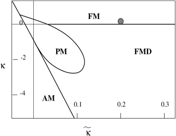
Figure 1: Schematic quenched phase diagram.

In the quenched approximation, we have first numerically confirmed the phase diagram in [11] of the reduced model in ($\kappa,\tilde{\kappa}$) plane. The phase diagram shown schematically in Fig.1 has the interesting feature that for large enough $\tilde{\kappa}$, there is a continuous phase transition between the broken phases FM and FMD. FMD phase is characterized by loss of rotational invariance and the continuum limit is to be taken from the FM side of the transition. In the full theory with gauge fields, the gauge symmetry reappears at this transition and the gauge boson mass vanishes, but the longitudinal gauge dof remain decoupled. In Fig.1 PM is the symmetric phase and AM is the broken anti-ferromagnetic phase. The numerical details involved in reconstruction of the phase diagram and the fermionic measurements that follow will be available in [7].

For calculating the fermion propagators, as in [4] we have chosen the point $\kappa=0.05$, $\tilde{\kappa}=0.2$ (gray blob in Fig.1). Although this point is far away from $\tilde{\kappa}=\infty$, around which we did our perturbation theory in the previous section, the important issue here is to choose a point near the FM-FMD transition and away from the FM-PM transition. The results below show that for the fermion propagators there is excellent agreement between numerical results obtained at $\kappa=0.05$, $\tilde{\kappa}=0.2$ and perturbation theory.

Numerically on $4^{3}\times 16$ and $6^{3}\times 16$ lattices with $L_{s}=22$ and $m_{0}=0.5$ we look for chiral modes at the domain wall ($s=0$), the anti-domain wall ($s=11$), and at the waveguide boundaries ($s=5,6$ and $s=16,17$). Error bars in all the figures are smaller than the symbols.

Figure 2: Propagators at domain wall $s=0$ ($L_{s}=22$; a.p.b.c. in $L_{4}$, $y=1.0$).

Figs.2 and 3 show the $RR$ propagator $|S_{RR}|$ and the $LL$ propagator $|S_{LL}|$ at the domain and anti-domain wall as a function of a component of momentum $p_{4}$ for both $\vec{p}=(0,0,0)$ (physical mode) and $(0,0,\pi)$ (first doubler mode) at $y=1$. From the figures, it is clear that the doubler does not exist, only the physical $RR$ ($LL$) propagator seems to have a pole at $p=(0,0,0,0)$ at the anti-domain (domain) wall. In all the figures, NS, PT and FF respectively indicate data from numerical simulation, from perturbation theory and from free fermion propagator by direct inversion of the free fermion matrix.

For Figs.2 and 3, PT also mean zeroth order perturbation theory, i.e., numerical solution of propagator following eq.(17). We have PT results also for $6^{3}\times 16$ lattice but have chosen not to show them because they fall right on top of the numerical data. Instead PT results shown for $8^{3}\times 20$ lattice for which the $p_{4}$ points are distinct. The dotted line in all figures refer to the propagator from PT using a $256^{3}\times 1024$ lattice. The curves stay the same irrespective of methods or lattice size. Based on the above, we can conclude that there are only free RH fermions at the anti-domain wall, and at the domain wall there are only free LH fermions.

Figure 3: Chiral propagators at domain wall $s=0$ ($L_{s}=22$; a.p.b.c. in $L_{4}$, $y=1.0$).

Figs.4 and 5 show no evidence of a chiral mode at the waveguide boundaries $s=5$ and 6 and excellent agreement with 1-loop perturbation theory. Here too doublers do not exist. Actually the agreement with the FF method (direct inversion of the free domain wall fermion matrix on a given finite lattice) is also excellent, because the 1-loop corrections are almost insignificant. For clarity, in Figs.4 and 5 we have not shown the $LL$ propagator on $s=5$ and the $RR$ propagator at $s=6$, but conclusions are the same.

Figure 4: $RR$-propagator at waveguide boundary $s=5$ ($L_{s}=22$, a.p.b.c. in $L_{4}$, $y=1.0$).

Figure 5: $LL$-propagator at waveguide boundary $s=6$ ($L_{s}=22$, a.p.b.c. in $L_{4}$, $y=1.0$).

Similar investigation at the other waveguide boundary $s=16,17$ also does not show any chiral modes. Previous investigations of the domain wall waveguide model without gauge fixing [5] have shown that the waveguide boundaries are the most likely places to have the unwanted mirror modes. This is why we have mostly concentrated in showing that there are no mirror chiral modes at these boundaries, although we have looked for chiral modes everywhere along the flavor dimension. In fact, we do not see any evidence of a chiral mode anywhere other than at the domain wall and the anti-domain wall.

5 Numerical results at $y\ll 1$

At $y=0$, the domain wall and the anti-domain wall are detached from each other. Fermion current considerations and numerical simulations clearly show in this case that mirror chiral modes form at the waveguide boundaries.

On the other hand, at $y=1$ (as presented above) and $y>1$ [12], the mirror chiral modes are certainly absent at the waveguide boundaries. Actually in this case, the only chiral modes are at the domain wall and at the anti-domain wall and the spectrum is that of a free domain wall fermion.

The interesting question is what happens at $y$ smaller than unity, especially at positive values near zero. To investigate this question, we looked for chiral modes at $y=0.75,\,0.5,\,0.25$ at places other than the domain wall and the anti-domain walls, especially at the waveguide boundaries. On a $6^{3}\times 16$ lattice, the chiral propagators at the waveguide boundaries showed an increasing trend as the fourth component of momentum $p_{4}$ (with $\vec{p}=\vec{0}$) was decreased to the minimum value possible for this lattice size, something that could signify a pole at zero momentum. To resolve this we took lattice sizes which were bigger in the 4-direction to accommodate lower $p_{4}$-values. We found that for each $y<1$ there is a big enough lattice size for which the chiral propagators ultimately start showing a descending trend. Obviously the smaller the Yukawa coupling, the bigger the $L_{4}$ extension was required. Moreover, all the chiral propagators at these small Yukawa couplings matched exactly with the corresponding free case. Our results at the waveguide boundaries $s=5,\,6$ are summarized in the Figs.6 and 7 for the $RR$ and the $LL$ propagators respectively. Poles for these chiral propagators are clearly not seen.

6 Conclusion

Using the gauge fixing approach and tuning only a finite number of counterterms (in this case, just the $\kappa$-term), we end up in the reduced model with free domain wall fermion theory consisting only of LH and RH chiral modes respectively at the domain and the anti-domain wall. With the U(1) transverse gauge dof back on the waveguide, only the RH fermions on the anti-domain wall will be gauged (according to our construction). The gauge degrees of freedom are completely decoupled.

We reached our conclusions for the case of $y=1$ by performing a perturbation theory for the fermion propagators around $\tilde{\kappa}=\infty$ and comparing them to the numerical results at $\tilde{\kappa}=0.2$. The comparison is near perfect due to the robust properties of domain wall fermions (this does not happen nearly as nicely for the Wilson fermions) and shows that as long as $\tilde{\kappa}$ is big enough to avoid the FM-PM transition, it is as good as infinity, i.e., the whole FM-FMD transition line is in the same universality class as the perturbation point $\tilde{\kappa}=\infty$.

Investigations at $y\ll 1$ lead to the same qualitative conclusions and indicate that the model for any nonzero Yukawa coupling belongs to one universality class.

The transition to a nonabelian gauge group in this gauge-fixing approach is nontrivial and should be pursued. A more detailed account of our studies can be found in [6, 7].

The authors thank M.F.L. Golterman, Y. Shamir, P.B. Pal and K. Mukherjee for useful discussions. One of the authors (SB) thanks the Theory Group and Computer Section, SINP for providing facilities.

Figure 6: RR propagator at waveguide boundary $s=5$ with (a) $y=0.25$, (b) $y=0.50$, (c) $y=0.75$, (d) $y=1.0$ ($L_{s}=22$; a.p.b.c. in $L_{4}$).

Figure 7: LL propagator at waveguide boundary $s=6$ with (a) $y=0.25$, (b) $y=0.50$, (c) $y=0.75$, (d) $y=1.0$ ($L_{s}=22$; a.p.b.c. in $L_{4}$).

References

- [1] Y. Shamir, Phys. Rev. D57 (1998) 132; M.F.L. Golterman, Y. Shamir, Phys. Lett. B399 (1997) 148
- [2] H. Neuberger, Phys. Lett. B183 (1987) 337
- [3] W. Bock et. al., hep-lat/9911005
- [4] W. Bock, M.F.L. Golterman, Y. Shamir, Phys. Rev. Lett 80 (1998) 3444
- [5] M.F.L. Golterman, K. Jansen, D.N. Petcher and J.C. Vink, Phys. Rev. D49 (1994) 1606
- [6] S. Basak and Asit K. De, hep-lat/9911029
- [7] S. Basak and Asit K. De, in preparation
- [8] D.B. Kaplan, Phys. Lett. B288 (1992) 342
- [9] W. Bock et. al., Phys. Rev. D58 (1998) 34501
- [10] S. Aoki, H. Hirose, Phys. Rev. D54 (1996) 3471
- [11] W. Bock et. al., Phys. Rev. D58 (1998) 54506
- [12] S. Basak, Asit K. De, Nucl. Phys. B (Proc. Suppl.) 83-84 (2000) 615