Domain wall fermion calculation of nucleon $g_{{}_{A}}/g_{{}_{V}}$

Abstract

We present a preliminary domain-wall fermion lattice-QCD calculation of isovector vector and axial charges, $g_{{}_{V}}$ and $g_{{}_{A}}$, of the nucleon. Since the lattice renormalizations, $Z_{{}_{V}}$ and $Z_{{}_{A}}$, of the currents are identical with DWF, the lattice ratio $(g_{{}_{A}}/g_{{}_{V}})^{\rm lattice}$ directly yields the continuum value. Indeed $Z_{{}_{V}}$ determined from the matrix element of the vector current agrees closely with $Z_{{}_{A}}$ from a non-perturbative renormalization study of quark bilinears. We also obtain spin related quantities $\Delta q/g_{{}_{V}}$ and $\delta q/g_{{}_{V}}$.

The isovector vector and axial charges, $g_{{}_{V}}$ and $g_{{}_{A}}$, of the nucleon provide an interesting additional test of the domain wall fermion (DWF) method in the baryon sector where it has succeeded in reproducing the mass difference between the positive- and negative-parity ground states, $N(939)$ and $N^{*}(1535)$ [1]. These charges are defined as

$$g_{{}_{V}}=G_{{}_{F}}\lim_{q^{2}\rightarrow 0}g_{{}_{V}}(q^{2})$$

from the isovector vector current $\langle n|V^{-}_{\mu}(x)|p\rangle$=

$$i\bar{u}_{n}[\gamma_{\mu}g_{{}_{V}}(q^{2})+q_{\lambda}\sigma_{\lambda\mu}g_{{}_{M}}(q^{2})]u_{p}e^{-ipx},$$

$${\rm and}\,\,g_{{}_{A}}=G_{{}_{F}}\lim_{q^{2}\rightarrow 0}g_{{}_{A}}(q^{2})$$

with the axial current $\langle n|A^{-}_{\mu}(x)|p\rangle$=

$$i\bar{u}_{n}\gamma_{5}[\gamma_{\mu}g_{{}_{A}}(q^{2})+q_{\mu}g_{{}_{P}}(q^{2})]u_{p}e^{-ipx}.$$

The values of $g_{{}_{V}}=G_{{}_{F}}\cos\theta_{c}$ and $g_{{}_{A}}/g_{{}_{V}}=1.2670(35)$ are well known from neutron $\beta$ decay. Here $G_{{}_{F}}$ denotes the Fermi constant and $\theta_{c}$ the Cabibbo angle. $g_{{}_{V}}=G_{{}_{F}}\cos\theta_{c}$ follows from vector current conservation. In contrast the axial current should receive a strong correction from quantum chromodynamics (QCD), resulting in the deviation of the ratio $g_{{}_{A}}/g_{{}_{V}}$ from unity.

In lattice calculations in general the two relevant currents get renormalized by the lattice cutoff. With conventional fermion schemes this renormalization usually makes the calculations rather difficult, if not intractable, even for such simple quantities like $g_{{}_{V}}$ and $g_{{}_{A}}$. However with DWF it is greatly simplified because $Z_{{}_{A}}=Z_{{}_{V}}$[2], so that the evaluation $g_{{}_{A}}^{\rm lattice}/g_{{}_{V}}^{\rm lattice}$ directly yields the continuum value.

Phenomenological models of baryons have not been successful in reproducing this ratio: the non-relativistic quark model gives a value of $5/3$, and the MIT bag model 1.07. Lattice calculations typically underestimate $g_{{}_{A}}$ by 20 % [4]. All of these previous lattice calculations are done with (improved) Wilson fermions and consequently suffer from $Z_{{}_{A}}\neq Z_{{}_{V}}$ and other renormalization complications.

The present numerical calculations use the same gauge configurations reported in ref. [3], the notations of which we follow here. From this work we know DWF works well. In particular: 1) fermion near-zero mode effects are well understood, 2) small chiral symmetry breaking induced by the finite extra dimension is described by a single parameter $m_{\rm res}$ in low-energy effective lagrangian, which decreases as $\beta$ or $L_{s}$ increases, with the value of $m_{\rm res}/m_{\rm strange}=0.033(3)$ at $\beta=6.0$ and $L_{s}=16$, and 3) non-perturbative renormalization (NPR) works well for the quark bilinears [2].

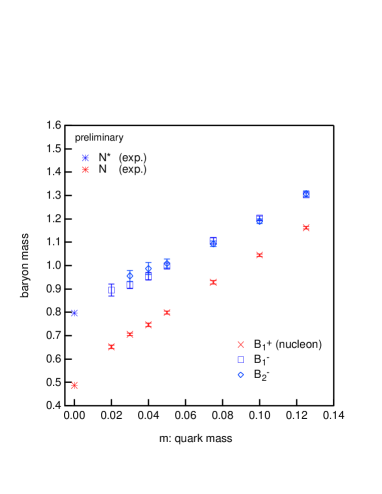
Figure 1: Dependence of $N$ (cross) and $N^{*}$ (square and diamond) mass on quark mass, $m_{f}$. Blasts at $m_{f}$=0 are experimental values in lattice unit, $a^{-1}$$\simeq$2 GeV.

Positive-parity nucleon states are created (destroyed) with interpolating operators $B_{1}^{+}=\epsilon_{abc}(u_{a}^{T}C\gamma_{5}d_{b})u_{c}$ and $B_{2}^{+}=\epsilon_{abc}(u_{a}^{T}Cd_{b})\gamma_{5}u_{c}$ while the negative-parity ones are created with $B_{1}^{-}=\gamma_{5}B_{1}^{+}=\epsilon_{abc}(u_{a}^{T}C\gamma_{5}d_{b})\gamma_{5}u_{c}$ and $B_{2}^{-}=\gamma_{5}B_{2}^{+}=\epsilon_{abc}(u_{a}^{T}Cd_{b})u_{c}$ with appropriate boundary conditions in time to reduce backward propagating contamination [1]. $B_{1}^{+}$ gives the ground-state nucleon ($N(939)$) mass. On the other hand $B_{2}^{+}$ seems to give the first excited positive parity state for heavier bare quark mass $m_{f}$. Whether it can reproduce the $N^{\prime}(1440)$ mass in the chiral limit is not yet known. $B_{1}^{-}$ and $B_{2}^{-}$ masses agree with each other, and yield the negative-parity ground state, $N^{*}(1535)$. Our quenched DWF calculation reproduces very well this large mass splitting between $N(939)$ and $N^{*}(1535)$ parity partners (see Figure 1). Phenomenological models like the non-relativistic quark model and the MIT bag model have failed here. It should be also noted that an earlier quenched lattice calculation using Wilson fermions [5] failed here too, though more recent calculations show improvements [6].

So DWF calculation of nucleon matrix elements seems promising. $g_{{}_{A}}$ is interesting because it is particularly clean with DWF since $Z_{{}_{A}}$=$Z_{{}_{V}}$. It is also interesting to see how well quenched calculations work for a well-known example of soft-pion behavior, namely the Goldberger-Treiman relation: $g_{{}_{A}}/g_{{}_{V}}$$\simeq$$f_{\pi}g_{\pi{{}_{N}}{{}_{N}}}/m_{{}_{N}}$$\simeq 1.31$. We know that with DWF the ratio $f_{\pi}/m_{{}_{N}}$ is almost constant over the range of $m_{f}$ we are using, and agrees well with the experimental value [3].

We follow the standard practice [4] for our two- and three-point function calculations. The two-point function is defined by

$$G_{{}_{{}_{N}}}(t)={\rm Tr}[(1+\gamma_{t})\sum_{\vec{x}}\langle TB_{1}(x)B_{1}(0)\rangle],$$

using $B_{1}=\epsilon_{abc}(u_{a}^{T}C\gamma_{5}d_{b})u_{c}$ for the proton. The three-point function for the local vector current is $G_{{}_{V}}^{u,d}(t,t^{\prime})$,

$${\rm Tr}[(1+\gamma_{t})\sum_{\vec{x}^{\prime},\vec{x}}\langle TB_{1}(x)V_{t}^{u,d}(x^{\prime})B_{1}(0)\rangle],$$

and for the local axial current, $G_{{}_{A}}^{u,d}(t,t^{\prime})$,

$${\rm Tr}[(1+\gamma_{t})\gamma_{i}\gamma_{5}\sum_{\vec{x}^{\prime},\vec{x}}\langle TB_{1}(x)A_{i}^{u,d}(x^{\prime})B_{1}(0)\rangle],$$

averaged over $i=x,y,z$. We choose a fixed $t=t_{\rm source}-t_{\rm sink}$ and $t^{\prime}<t$. From their lattice estimates

$$g_{{}_{\Gamma}}^{\rm lattice}=\frac{G_{{}_{\Gamma}}^{u}(t,t^{\prime})-G_{{}_{\Gamma}}^{d}(t,t^{\prime})}{G_{{}_{{}_{N}}}(t)},$$

with $\Gamma=V$ or $A$, the continuum values

$$g_{{}_{\Gamma}}=Z_{{}_{\Gamma}}g_{{}_{\Gamma}}^{\rm lattice},$$

are obtained. Here we need the non-perturbative renormalizations, defined by

$$[\bar{u}\Gamma d]_{\rm ren}=Z_{{}_{\Gamma}}[\bar{u}\Gamma d]_{0},$$

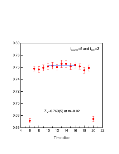
Figure 2: Dependence of vector renormalization, $Z_{{}_{V}}=1/g_{{}_{V}}^{\rm lattice}$, on $t^{\prime}$, at $m_{f}=0.02$. A good plateau is observed.

which should satisfy $Z_{{}_{A}}=Z_{{}_{V}}$ so that

$$\left(\frac{g_{{}_{A}}}{g_{{}_{V}}}\right)^{\rm continuum}=\left(\frac{G_{{}_{A}}^{u}(t,t^{\prime})-G_{{}_{A}}^{d}(t,t^{\prime})}{G_{{}_{V}}^{u}(t,t^{\prime})-G_{{}_{V}}^{d}(t,t^{\prime})}\right)^{\rm lattice}.$$

Note $g_{{}_{A}}$ is described as $\Delta u-\Delta d$ where $\Delta f$ ($f=u$ or $d$) is defined by

$$\langle p,s|\bar{f}\gamma_{5}\gamma_{\mu}f|p,s\rangle=2s_{\mu}\Delta q,$$

with $s$ satisfying $s\cdot p=0$ and $s^{2}=-1$. From these we obtain spin-polarized longitudinal parton distribution, $\Delta q=\int dx[q_{\uparrow}(x)-q_{\downarrow}(x)]=\Delta u+\Delta d$. Similarly, $\delta f$ is defined by

$$\langle p,s|i\bar{f}\sigma_{\mu\nu}\gamma_{5}f|p,s\rangle=2(s_{\mu}p_{\nu}-s_{\nu}p_{\mu})\delta f,$$

with $\sigma_{\mu\nu}=[\gamma_{\mu},\gamma_{\nu}]/2$. This gives the tensor charge which is related to the transverse parton distribution, $\delta q=\int dx[q_{\bot}(x)-q_{\top}(x)]=\delta u+\delta d$. We define $G_{{}_{T}}^{q}(t,t^{\prime})$ by inserting $T_{i}^{q}=\bar{q}\gamma_{t}\gamma_{i}\gamma_{5}q$ at $t^{\prime}$ and a projection operator $(1+\gamma_{t})\gamma_{i}\gamma_{5}$, and

$$\delta q^{\rm lattice}=\frac{G_{{}_{T}}^{u}(t,t^{\prime})+G_{{}_{T}}^{d}(t,t^{\prime})}{G_{{}_{N}}(t)}$$

is obtained. Here we need $Z_{{}_{T}}$, which is scheme- and scale-dependent. Note that $\Delta u=\delta u=4/3$ and $\Delta d=\delta d=-1/3$ in the heavy quark limit.

The numerical calculations are from 200 configurations at $\beta=6.0$ on a $16^{3}\times 32$ lattice with DWF parameters $L_{s}=16$ and $M_{5}=1.8$. We set the source at $t=5$, sink at 21, and current insertions in between. The vector renormalization, $Z_{{}_{V}}=1/g_{{}_{V}}^{\rm lattice}$, is well-behaved,

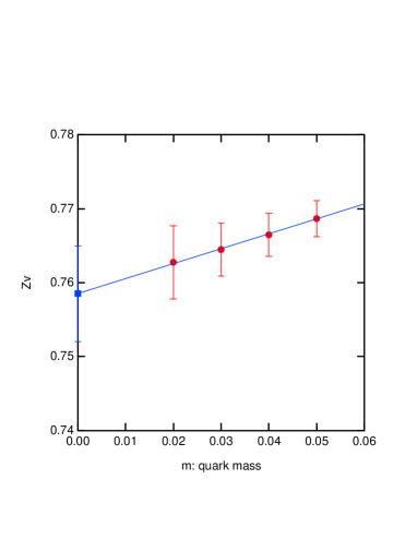
Figure 3: Dependence of vector renormalization, $Z_{{}_{V}}=1/g_{{}_{V}}^{\rm lattice}$, on $m_{f}$. Note the scale. Slight linear dependence extrapolates to the value of 0.759(6) at $m_{f}$=0.

The value $0.763(5)$ at $m_{f}=0.02$ (See Figure 2) agrees well with $Z_{{}_{A}}=0.7555(3)$, obtained from $\langle A^{\rm conserved}_{\mu}(t)\bar{q}\gamma_{5}q(0)\rangle=Z_{{}_{A}}\langle A^{\rm local}_{\mu}(t)\bar{q}\gamma_{5}q(0)\rangle$ [3]. A linear extrapolation gives $Z_{{}_{V}}=0.759(6)$ at $m_{f}=0$ (Figure 3). For the lattice axial charge, $g_{{}_{A}}^{\rm lattice}$, plateaus are seen for $10\leq t\leq 16$, with a fairly strong dependence on $m_{f}$ (See for example Figure 4). So the charge ratio, $g_{{}_{A}}/g_{{}_{V}}$, averaged in $10\leq t\leq 16$,

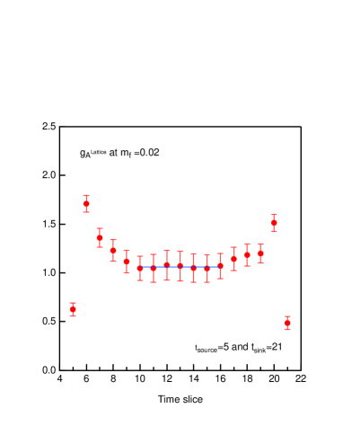
Figure 4: The lattice axial charge, $g_{{}_{A}}^{\rm lattice}$, at $m_{f}=0.02$. A good plateau is seen in $10\leq t\leq 16$.

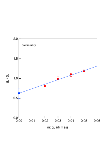
Figure 5: Dependence of $g_{{}_{A}}/g_{{}_{V}}$ on $m_{f}$.

linearly extrapolates to 0.62(13) at $m_{f}=0$ (Figure 5) which is about a factor of 2 smaller than experiment. However a linear fit may not be justified here. There is some curvature apparent in Figure 5, so the value of $g_{{}_{A}}/g_{{}_{V}}$ in the chiral limit may be even lower. The same calculation yields (with linear extrapolations to $m_{f}=0$) $\Delta u/g_{{}_{V}}=0.50(12)$ and $\Delta d/g_{{}_{V}}=-0.14(6)$. Similarly, $\delta u/g_{{}_{V}}=0.39(11)$ and $\delta d/g_{{}_{V}}=-0.11(4)$. A preliminary value for $Z_{{}_{T}}/Z_{{}_{A}}$ is 1.1(1) [2].

In summary we have explored the isovector weak interaction of the nucleon in lattice QCD with domain-wall fermions. All the relevant three-point functions are well behaved. $Z_{{}_{V}}$ determined from the matrix element of the vector current agrees closely with that from an NPR study of quark bilinears [2]. Linear extrapolations to $m_{f}$=0 give

• $g_{{}_{A}}/g_{{}_{V}}=0.62(13)$,

• $\Delta q/g_{{}_{V}}=0.36(14)$,

• $\delta q/g_{{}_{V}}=0.31(12)$.

The quite low value of $g_{{}_{A}}/g_{{}_{V}}$ that we obtained requires further investigation. In particular, we are studying the Ward-Takahashi identity which governs $g_{{}_{A}}$. If the matrix element of the pseudoscalar density does not develop a pole as $m_{f}\to 0$ which is expected in the Goldberger-Treiman relation, the left hand side, and therefore $g_{{}_{A}}$, must vanish. Further study is also required to check systematic errors arising from finite lattice volume, excited states (small separation between $t_{\rm source}$ and $t_{\rm sink}$), and quenching (zero modes, absent pion cloud, etc), especially in the lighter quark mass region.

References

[1] S. Sasaki, in Proc. NSTAR 2000, hep-ph/0004252.
[2] C. Dawson, in these proceedings and C. Dawson et al,
private communication.
[3] T. Blum et al (RBC Collaboration), hep-lat/0007038,
to appear in Phys. Rev. D.
[4] M. Fukugita et al, Phys. Rev. Lett. 75, 2092 (1995);
S.J. Dong et al, Phys. Rev. Lett. 75, 2096 (1995);
K.F. Liu et al, Phys. Rev. D49, 4755 (1994);
M. Göckeler et al, Phys. Rev. D53, 2317 (1996);
S. Capitani et al,
in Proc. Lattice 98, Nucl. Phys. B (Proc. Suppl.) 73, 294 (1999);
S. Capitani et al,
Proc. DIS 99, Nucl. Phys. B (Proc. Suppl.) 79, 548 (1999);
S. Güsken et al,
Phys. Rev. D59, 114502 (1999).
[5] F.X. Lee and D.B. Leinweber, in Proc. Lattice 98,
Nucl. Phys. B (Proc. Suppl.) 73, 258 (1999).
[6] D. Richards, in these proceedings; F.X. Lee, in
these proceedings.