Towards the application of the Maximum Entropy Method to finite temperature Upsilon Spectroscopy

Abstract

According to the Narnhofer Thirring Theorem [1] interacting systems at finite temperature cannot be described by particles with a sharp dispersion law. It is therefore mandatory to develop new methods to extract particle masses at finite temperature. The Maximum Entropy method offers a path to obtain the spectral function of a particle correlation function directly. We have implemented the method and tested it with zero temperature $\Upsilon$ correlation functions obtained from an NRQCD simulation. Results for different smearing functions are discussed.

1 Introduction

With $J/\Psi$-suppression being one of the key probes for the quark gluon plasma [2] a nonperturbative understanding of heavy quarkonia at temperatures above the transition temperature is important. The extraction of particle masses at finite temperature is aggravated on a practical level by the compactified Euclidean time direction and on a more fundamental level by the Narnhofer Thirring theorem. One has to employ methods that do not make any assumptions about the spectral structure. A zero momentum Euclidean current current correlator $G(\tau)$ has the following spectral representation [3]:

$$G(\tau)=\frac{1}{\pi}\int_{0}^{\infty}\frac{\cosh((\frac{\beta}{2}-\tau)\omega)}{\sinh(\frac{\beta}{2}\omega)}\rho(\omega)d\omega$$ (1)

The (temperature dependent) spectral function $\rho(\omega)$ contains all the real-time physics information we are interested in. Indeed the Fourier transform of the retarded correlator is given in terms of the spectral function as

$$\tilde{G}_{R}(\omega)=\frac{1}{\pi}\int_{-\infty}^{\infty}\frac{\rho(\omega^{\prime})}{\omega+i\epsilon-\omega^{\prime}}d\omega^{\prime}$$

Extraction of $\rho(\omega)$ from Eq.(1) by inversion is numerically an ill-posed problem [4] and the Maximum Entropy method can be seen as a regularization of this ill-posed problem, but has in fact a deeper justification from Bayesian statistics.

2 The Maximum Entropy Method

The Maximum Entropy method (MEM) is a well known technique for image reconstruction and has been successfully applied in astronomy and condensed matter physics. For a review see [5]. MEM is based on Bayesian methods of inference which in turn centers around Bayes theorem of conditional probabilities, which in our case reads:

$$P\left[\rho|G,I\right]\sim P\left[G|\rho,I\right]P\left[\rho|I\right]$$ (2)

where $\rho$ is the spectral function, G are the data for the correlator and I is any a priori information that is relevant to the problem. $P\left[G|\rho,I\right]$ is called the likelihood and is proportional to $\exp(-L)$ for a large number of measurements with

$$L=\frac{1}{2}\chi^{2}=\frac{1}{2}\sum_{i,j}^{N_{\tau}}(F(\tau_{i})-G(\tau_{i})C_{i,j}^{-1}(F(\tau_{j})-G(\tau_{j}))$$

$C_{i,j}$ being the covariance matrix and $F(\tau)=\int K(\tau,\omega)\rho(\omega)d\omega$ is the ’fit function’ in terms of the spectral density $\rho(\omega)$ and the kernel $K(\tau,\omega)$ defined by Eq(1). $P\left[\rho|I\right]$ is the prior probability for the spectral function. Using Bayesian lines of thought [6] one can show that the prior probability is of entropic form $\exp(-\alpha S)$.

$$S=\int[\rho(\omega)-m(\omega)-\rho(\omega)\log(\frac{\rho(\omega)}{m(\omega)})]d\omega$$

$m(\omega)$ is a default model with respect to which we measure the entropy of the spectral function. The freedom to choose a default model can be used to incorporate further knowledge, but trustable results should not depend on $m(\omega)$. We choose $m(\omega)\sim\omega^{2}$, which is the perturbative high energy form of mesonic spectral functions [7, 8]. The real and positive parameter $\alpha$ controls the relative weight between the entropy and the the likelihood. In the algorithm used here to determine the spectral function [9] $\alpha$ is eliminated by marginalization. A detailed analysis shows that one can determine the probability $P\left[\alpha|G\right]$ from the data. And the final result is then given as a weighted average over $\hat{\rho}_{\alpha}(\omega)$ which is the spectral function that maximises $Q=\alpha S-L$, i.e. maximises the conditional probability $P\left[\rho|G,I\right]$ in Eq.(2):

$$\bar{\rho}(\omega)=\int\hat{\rho}_{\alpha}(\omega)P\left[\alpha|G\right]d\alpha$$

The maximization of $Q$ over the space of $\rho$ makes use of a Singular Value Decomposition of the kernel $K(\tau,\omega)$, by expressing $\rho$ in terms of the singular vectors of $K$. In this way the algorithm chooses the appropriate degrees of freedom of which there are, by construction, always fewer than the number of timeslices. MEM therefore makes no assumption about the spectral shape except for that which is dictated by the the discretisation of the kernel.

3 Testing MEM with $\Upsilon$ data

Since we are ultimately interested in studying the melting of $\Upsilon$ and $J/\Psi$ above the critical temperature, we have tested the method with data from a precision $\Upsilon$ spectroscopy study at zero temperature using NRQCD reported in [10]. We have analyzed local and smeared correlation functions in the ${}^{3}S_{1}$-channel with Richardson potential radial wave functions for the smearings. The smearings at source and sink have to be identical for Eq.(1) to hold. Fig.1 shows our results.

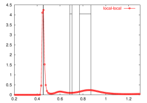
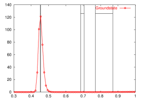
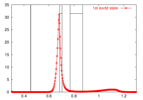
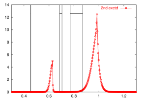
Figure 1: Spectral functions $\rho(\omega)/\omega^{2}$ for (top to bottom) the local-local correlator, ground-state smearing, 1st excited state smearing, 2nd excited state smearing. The vertical lines indicate the error-bands of the results of [10].

In all graphs we plot $f(\omega)=\rho(\omega)/\omega^{2}$ to divide out the assumed default model $m(\omega)=0.1\omega^{2}$. The integration in Eq.(1) is performed up to $\omega_{max}=7.5>2\pi$. The results do not depend on $\omega_{max}$ as long as $\omega_{max}>2\pi$, the maximum lattice momentum of the meson. We only show the spectral function up to $\omega\sim 1.2$, since $f(\omega)$ is virtually zero beyond this value except for $\omega$ close to $\omega_{max}$ when $f(\omega)$ tends to $0.1$, the default model value. The data do not contain enough information to constrain the spectral function at such high momenta. The results also do not depend on the discretisation $d\omega$ as long as $d\omega$ is smaller than the finest structure that is contained in the data. These results have been produced with $d\omega=0.01$. We have also checked the independence of our results from the default model. We have varied the prefactor of $\omega^{n}$ between 0.002 and 5.0 and the power $n$ of $\omega^{n}$ between 0 and 3.

3.1 Discussion of the results

The local-local correlator shows a clear ground-state peak at the location expected from the analysis in [10]. There is some indication for spectral strength of excited states, but the shape is not very pronounced. Similar behaviour has been reported in [7, 8]. What is new here is the analysis of smeared correlators. Although a smeared correlation function probes the same quantum numbers as the local correlator, the shape of the spectral function of a smeared operator will in general be different from the local spectral function. However the position of a peak in the spectral function should not be affected by smearing. The second plot of Fig.1 shows the result for ground-state smearing and indeed one finds a clear peak with no indication of any excited states. The next plot is the smearing for the first excited state. The peak position is consistent with the results from the standard analysis. There is no contamination from the ground-state and only a slight indication of higher excited states. For the last plot a comment is in order. We have not said anything so far about the statistical significance of our results and if we take the last plot at face value it presents us with a problem. The lower of the two peaks lies lower than the result for the first excited state. Either the 1st excited state smearing did in fact project onto a higher state and this is the true first excited state or something is problematic with the 2nd excited state smearing. The second peak which we expect to be the second excited state lies higher than the result from the correlated matrix fit of [10]. The large error band from the standard analysis already indicates that this state is difficult to analyse. The error analysis described in the next section indicates that both peak positions are in fact compatible with the results of [10] and that the data for this smearing are probably not good enough to pin down this state. One expects that higher excited states become more and more visible as one increases $N_{\tau}$, the number of points in the time direction. At finite temperature it will therefore be advisable to use anisotropic lattices in order to have large $N_{\tau}>24$ at still manageable spatial lattice sizes.

3.2 Rotated smearings

Suppose one has a set of smearings $\left.|0\right>,\left.|1\right>,\left.|2\right>...$. Measuring all cross correlators $\left<0|0\right>,\left<0|1\right>,\left<1|0\right>...$, one can construct all correlators with smearings that can be expressed as linear superpositions of the original smearings: $\left.|\Psi\right>=\alpha_{0}\left.|0\right>+\alpha_{1}\left.|1\right>+\alpha_{2}\left.|2\right>+...$. The correlator $G(\tau)=\left<\Psi(\tau)|\Psi(0)\right>$ will then also have a spectral representation which can be analysed with our methods. Fig.2 is an example of such a procedure.
Figure 2. Spectral functions for 3 different superpositions of the ground-state and excited state smearings.

This could be used to construct optimised smearing functions that contained little or no contamination from unwanted states.

3.3 Error analysis

An important issue is of course the error analysis for MEM reconstructed spectral functions. One important point to note here is the fact that the spectral function is a density. It therefore does not make sense to assign errors to individual points, since different points are correlated because e.g. the normalization of $\rho$ is fixed. One can adopt an approach suggested in [5] in which the covariance of $\rho$ around the maximum of $Q$ is averaged over $\alpha$. This is an approach within the logic of Bayesian statistics. We have taken a more reserved approach and asked how robust is the MEM prediction under a change of sample. To investigate this we have created bootstrap samples from the original data and run the whole analysis for every such sample. For the ground-state smearing this procedure results in a stable prediction. The peak position does not change, only the shape of the peak. For the 1st excited state smearing the situation is still very good. The result of this analysis for the 2nd excited state smearing is displayed in Figure 3. It is clear from this figure that one cannot trust the result for this smearing.
Figure 3. Spectral functions for 10 bootstrap samples for the 2nd excited state smearing showing the variation in shape and position of the peaks. The dotted lines are errors of the peak position based on 10 bootstraps.

This shows that it is possible to investigate the statistical significance of MEM prediction by general bootstrap methods.

4 Conclusions

We have shown that with the Maximum Entropy method one has access to the spectral function of a current-current correlator which contains all the information about the excitation spectrum of the theory in the channel represented by this current. We have also shown that one has good access to excited states when smeared operators are used. In particular rotating correlators in a given basis of smearing functions, one can produce smearings which contain almost no contamination from unwanted states, complementing standard spectroscopy techniques. Since the method makes no assumptions about the shape of the spectral function, it can also be used at finite temperature where little is known about its structure except for the absence of single particle $\delta$-function peaks. We intend to use the method to investigate $\Upsilon$ and $J/\Psi$ melting above the critical temperature.

References

- [1] M. Requard H. Narnhofer and W. Thirring. Commun. Math. Phys. 92, 247 (1983).
- [2] H. Satz. these proceedings.
- [3] S. Huang. Phys. Rev. D 47, 653 (1993).
- [4] Ph. de Forcrand et. al. Nucl. Phys. B (Proc. Suppl.) 63A-C, 460 (1998).
- [5] M. Jarrel and J. E. Gubernatis. Phys. Rep. 269, 133 (1996).
- [6] J. Skilling. In Maximum Entropy and Bayesian Methods, editor J. Skilling. Kluwer Academic Publishers (1989).
- [7] Y. Nakahara et. al. Phys. Rev. D 60, 091503 (1999).
- [8] Y. Nakahara et. al. Nucl. Phys. B (Proc. Suppl.) 83-84, 191 (2000).
- [9] R. K. Bryan. Eur. Biophys. J. 18, 165 (1990).
- [10] C. T. H. Davies et. al. Phys. Rev. D 50, 6963 (1994).