CERN-TH/2000-226

NORDITA-2000/80HE

hep-lat/0009025

TWO HIGGS DOUBLET DYNAMICS AT THE ELECTROWEAK
PHASE TRANSITION: A NON-PERTURBATIVE STUDY

M. Laine^a,b, K. Rummukainen^c,d

^aTheory Division, CERN, CH-1211 Geneva 23, Switzerland
^bDept. of Physics, P.O.Box 9, FIN-00014 Univ. of Helsinki, Finland
^cNORDITA, Blegdamsvej 17, DK-2100 Copenhagen Ø, Denmark
^dHelsinki Inst. of Physics, P.O.Box 9, FIN-00014 Univ. of Helsinki, Finland

Using a three-dimensional (3d) effective field theory and non-perturbative lattice simulations, we study the MSSM electroweak phase transition with two dynamical Higgs doublets. We first carry out a general analysis of spontaneous CP violation in 3d two Higgs doublet models, finding that this part of the parameter space is well separated from that corresponding to the physical MSSM. We then choose physical parameter values with explicit CP violation and a light right-handed stop, and determine the strength of the phase transition. We find a transition somewhat stronger than in 2-loop perturbation theory, leading to the conclusion that from the point of view of the non-equilibrium constraint, MSSM electroweak baryogenesis can be allowed even for a Higgs mass $m_{H}\approx 115$ GeV. We also find that small values of the mass parameter $m_{A}$ ($\mathop{\raise 1.29167pt\hbox{$<$\kern-7.5pt\raise-4.73611pt\hbox{$\sim$}}}120$ GeV), which would relax the experimental constraint on $m_{H}$, do not weaken the transition noticeably for a light enough stop. Finally we determine the properties of the phase boundary.

CERN-TH/2000-226
NORDITA-2000/80HE
November 2000

1 Introduction

The observed existence of a baryon asymmetry in our Universe is direct evidence for physics beyond the Minimal Standard Model. Indeed, the electroweak theory contains anomalous baryon number violation which is rapid enough to be in thermal equilibrium at temperatures $T\mathop{\raise 1.29167pt\hbox{$>$\kern-7.5pt\raise-4.73611pt\hbox{$\sim$}}}100$ GeV [1, 2, 3, 4], so that any pre-existing asymmetry is washed out. (Unless there is an asymmetry in baryon minus lepton number, $B-L$, which would also require physics beyond the Minimal Standard Model; for an overview on recent scenarios based on this, see [5]). As the Universe then cools down, it turns out that there is no electroweak phase transition at all for Higgs masses $m_{H}\mathop{\raise 1.29167pt\hbox{$>$\kern-7.5pt\raise-4.73611pt\hbox{$\sim$}}}72$ GeV [6, 7, 8], or $m_{H}\mathop{\raise 1.29167pt\hbox{$>$\kern-7.5pt\raise-4.73611pt\hbox{$\sim$}}}90$ GeV in the presence of primordial magnetic fields [9]: the cosmological evolution is just smooth and continuous. Taking the experimental lower bound $m_{H}\mathop{\raise 1.29167pt\hbox{$>$\kern-7.5pt\raise-4.73611pt\hbox{$\sim$}}}110$ GeV into account [10] (the factual bound is even a few GeV higher by now), this would mean that the baryon symmetric high temperature state simply freezes in, in contradiction with observation.

It is quite interesting that already one of the simplest extensions of the Minimal Standard Model, the Minimal Supersymmetric Standard Model (MSSM), offers a definite and experimentally testable way of changing this conclusion. One can uniquely identify a bosonic degree of freedom, the right-handed stop, which can be “light” and dynamical at the phase transition point without violating experimental constraints at zero temperature, and interacts strongly enough with the Higgs to strengthen the phase transition significantly [11]–[23]. There are also new sources of CP violation available which could potentially have a favourable effect [24]–[28]. Many details of the electroweak phase transition in this region have recently been studied [29]–[36].

In this paper, we address several issues related to the electroweak phase transition in the MSSM. The first is CP violation in the background configuration related to the fact that there are two Higgs doublets. The second is the strength of the phase transition at an experimentally viable parameter point corresponding to a Higgs mass of about 105 GeV, not excluded for the MSSM with smallish $m_{A}$. (We also consider other values close to these, notably $m_{H}$ up to $\sim$ 115 GeV.) The third is the structure of the phase boundary, or bubble wall, at the physical parameter point.

In particular, as to the first of these issues, we will pay some attention to the phenomenon of spontaneous CP violation. Spontaneous CP violation can in principle take place in any two Higgs doublet model [37], but for the physical MSSM parameters it cannot be realized at $T=0$ [38, 39]. However, it has been suggested that it might be more easily realized at finite temperatures [40, 41], or even only in the phase boundary between the symmetric and broken phases [42, 43] (in which case it is sometimes called “transitional” CP violation). The existence of spontaneous CP violation would mean that even small explicit phases can have a large physical effect, and such a situation within the phase boundary would conceivably be useful for electroweak baryogenesis [44]–[48].

The method we use to study all the three questions is the construction of an effective 3d field theory with the method of dimensional reduction, and its non-perturbative analysis with simple lattice simulations. The dimensional reduction step was already carried out in [49], and here we concentrate on the non-perturbative part.

The plan of this paper is the following. In Sec. 2 we review briefly the form of the 3d effective field theory for the MSSM, arising after dimensional reduction. In Sec. 3 we discuss the lattice implementation of this theory — this section should be skipped by those not interested. In Sec. 4 we carry out a general analysis of the phase diagram of the 3d theory, with particular view on spontaneous CP violation. In Sec. 5 we focus on a physical choice of parameters and determine the strength of the phase transition, while in Sec. 6 we determine the properties of the phase boundary appearing in the physical transition, checking also for the possibility of transitional CP violation. We summarise and discuss implications in Sec. 7.

2 The effective theory

2.1 The action

At finite temperatures around the electroweak phase transition, the thermodynamics of the MSSM can be represented by a 3d effective field theory containing two SU(2) Higgs doublets $H_{1},H_{2}$ and one SU(3) stop triplet $U$ [49]. The action is of the most general gauge invariant form,

$${\cal L}_{\mbox{\scriptsize 3d}} = {\frac{1}{2}}{\rm Tr\,}G_{ij}^{2}+(D_{i}^{s}U)^{\dagger}(D_{i}^{s}U)+m_{U}^{2}(T)U^{\dagger}U+\lambda_{U}(U^{\dagger}U)^{2}$$ (2.1)

$$+ \gamma_{1}U^{\dagger}UH_{1}^{\dagger}H_{1}+\gamma_{2}U^{\dagger}UH_{2}^{\dagger}H_{2}+\Bigl{[}\gamma_{12}U^{\dagger}UH_{1}^{\dagger}\tilde{H}_{2}+{\rm H.c.\ }\Bigr{]}$$

$$+ {\frac{1}{2}}{\rm Tr\,}F_{ij}^{2}+(D_{i}^{w}H_{1})^{\dagger}(D_{i}^{w}H_{1})+(D_{i}^{w}H_{2})^{\dagger}(D_{i}^{w}H_{2})$$

$$+ m_{1}^{2}(T)H_{1}^{\dagger}H_{1}+m_{2}^{2}(T)H_{2}^{\dagger}H_{2}+\Bigl{[}m_{12}^{2}(T)H_{1}^{\dagger}\tilde{H}_{2}+{\rm H.c.\ }\Bigr{]}$$

$$+ \lambda_{1}(H_{1}^{\dagger}H_{1})^{2}+\lambda_{2}(H_{2}^{\dagger}H_{2})^{2}+\lambda_{3}H_{1}^{\dagger}H_{1}H_{2}^{\dagger}H_{2}+\lambda_{4}H_{1}^{\dagger}\tilde{H}_{2}\tilde{H}_{2}^{\dagger}H_{1}$$

$$+ \Bigl{[}\lambda_{5}(H_{1}^{\dagger}\tilde{H}_{2})^{2}+\lambda_{6}H_{1}^{\dagger}H_{1}H_{1}^{\dagger}\tilde{H}_{2}+\lambda_{7}H_{2}^{\dagger}H_{2}H_{1}^{\dagger}\tilde{H}_{2}+{\rm H.c.\ }\Bigr{]}.$$

Here $D_{i}^{s},D_{i}^{w}$ are the spatial SU(3) and SU(2) covariant derivatives, $G_{ij},F_{ij}$ the corresponding field strength tensors, and $\tilde{H}_{2}=i\sigma_{2}H_{2}^{*}$. We denote the SU(3) and SU(2) gauge couplings by $g_{s},g_{w}$. We have neglected the dynamical effects of the U(1) subgroup since they are expected to be small [50] (although some aspects of the system with a dynamical U(1) remain to be understood [51]). Note also that compared with the MSSM, $U$ denotes the complex conjugate of the original right-handed stop triplet. The couplings in Eq. (2.1) can be expressed in terms of the physical parameters of the MSSM and the temperature $T$, as will be specified below.

For future reference, let us recall that if one is only interested in the strength of the phase transition, the effective theory in Eq. (2.1) is even unnecessarily complicated. Indeed, it is easy to understand [52, 14, 15, 16, 17, 49] (see also Appendix A) that if the two Higgs doublet mass matrix is diagonalized, one of the eigendirections is always heavy, and can be perturbatively integrated out. This results in an effective theory with a single SU(2) Higgs doublet, and the right-handed stop. We studied that effective theory with lattice simulations in [19]. The reason we keep here both Higgs doublets is that we measure a number of observables which are specific to the existence of both fields, and cannot be addressed with the simpler theory.

The couplings appearing in the 3d theory in Eq. (2.1) have the dimension GeV, and the fields have the dimension GeV^1/2. For later convenience, we will parameterise the couplings by introducing what from the point of view of the 3d theory is an arbitrary scale, the temperature $T$. We then scale all the couplings to a dimensionless form by dividing with $T$, and all the fields into a dimensionless form by dividing with $T^{1/2}$:

$$g^{2}\equiv\frac{g_{\mbox{\scriptsize 3d}}^{2}}{T},\quad\lambda_{i}\equiv\frac{\lambda_{i,{\mbox{\scriptsize 3d}}}}{T},\quad\gamma_{i}\equiv\frac{\gamma_{i,{\mbox{\scriptsize 3d}}}}{T},\quad\frac{H_{i}}{T}\equiv\frac{H_{i,{\mbox{\scriptsize 3d}}}}{T^{1/2}},\quad\frac{U}{T}\equiv\frac{U_{{\mbox{\scriptsize 3d}}}}{T^{1/2}}.$$ (2.2)

Expressed in terms of the newly defined coupling constants and fields, the action goes over into

$$S=\int\!d^{3}x\,{\cal L}_{\mbox{\scriptsize 3d,orig}}\to\frac{1}{T}\int\!d^{3}x\,{\cal L}_{\mbox{\scriptsize 3d}},$$ (2.3)

where the dimensionality of the new ${\cal L}_{\mbox{\scriptsize 3d}}$ is GeV⁴ as usually in 4d. We shall use this formulation throughout the paper, with $T$ taken to be the physical temperature.

2.2 Approximate physical values of couplings

Expressions for the parameters in Eq. (2.1), corresponding to the MSSM, have been derived in [49]; for a summary, see Appendix A.7 there. We cite the precise values used in Secs. 5, 6 later on, but let us recall the general orders of magnitude already here.

It is important to keep in mind a basic difference between the effective theories corresponding to the Standard Model and the MSSM. In the former, the physical Higgs mass is determined by the effective quartic scalar coupling, $\lambda\sim(g_{w}^{2}/8)(m_{H}^{2}/m_{W}^{2})$, while the temperature is determined by the 3d scalar mass parameter, $m_{\mbox{\scriptsize 3d}}^{2}(T)\sim-m_{H}^{2}/2+0.3T^{2}$. In the MSSM, on the contrary, the quartic Higgs couplings are fairly inert, $\sim g_{w}^{2}/8$, and are affected by the zero-temperature Higgs mass (i.e., by $\tan\beta$) only through small radiative corrections. Thus both the physical Higgs spectrum and the temperature reside now dominantly in the effective mass parameters. The rough generic orders of magnitude for the quartic couplings in the MSSM can therefore be cited [49], independent of the Higgs mass and temperature:

$$\lambda_{1}\sim 0.07,\quad\lambda_{2}\sim 0.13,\quad\lambda_{3}\sim 0.08,\quad\lambda_{4}\sim-0.22,$$ (2.4)

$$|\lambda_{5}|\mathop{\raise 1.29167pt\hbox{$<$\kern-7.5pt\raise-4.73611pt\hbox{$\sim$}}}0.002,\quad|\lambda_{6}|\mathop{\raise 1.29167pt\hbox{$<$\kern-7.5pt\raise-4.73611pt\hbox{$\sim$}}}0.01,\quad|\lambda_{7}|\mathop{\raise 1.29167pt\hbox{$<$\kern-7.5pt\raise-4.73611pt\hbox{$\sim$}}}0.02,$$ (2.5)

$$\lambda_{U}\sim 0.19,\quad g_{w}^{2}\sim 0.42,\quad g_{s}^{2}\sim 1.1.$$ (2.6)

In $\lambda_{1},\lambda_{3},\lambda_{4}$, we have included only the tree-level terms, but in $\lambda_{2}$ also the dominant 1-loop terms proportional to the top Yukawa coupling to the fourth power, $h_{t}^{4}$, which are absent in $\lambda_{1},\lambda_{3},\lambda_{4}$ (we recall that $h_{t}\approx 1.0$). In order to get the estimates for $\lambda_{5}...\lambda_{7}$, we have taken into account that when the right-handed stop is light, the squark mixing parameters cannot be too large compared with the left-handed stop mass, because of the stability of the theory (see below).

As to the three couplings $\gamma_{i}$ in Eq. (2.1), they can be reparameterised in terms of the three couplings $h_{t},\hat{A}_{t},\hat{\mu}$ as

$$\gamma_{1}=-h_{t}^{2}|\hat{\mu}|^{2},\quad\gamma_{2}=h_{t}^{2}(1-|\hat{A}_{t}|^{2}),\quad\gamma_{12}=h_{t}^{2}\hat{A}_{t}^{*}\hat{\mu}^{*},$$ (2.7)

where $A_{t},\mu$ are the mixing parameters in the 3rd generation squark mass matrix, $m_{Q}$ is the corresponding left-handed squark mass parameter, and $\hat{A}_{t}\approx A_{t}/m_{Q}$, $\hat{\mu}\approx\mu/m_{Q}$. There are of course radiative corrections to these relations, but we can also view them as a more general reparameterization, since $\hat{A}_{t},\hat{\mu}$ are essentially free parameters. We mostly assume $\hat{A}_{t},\hat{\mu}\mathop{\raise 1.29167pt\hbox{$<$\kern-7.5pt\raise-4.73611pt\hbox{$\sim$}}}0.3$, again in order not to destabilize the theory (see, e.g., [49]), and also since large values tend to weaken the phase transition (see, e.g., [13, 16, 20]).

Consider finally the mass parameters. Working in the limit $\tilde{m}_{U}^{2}\equiv-m_{U}^{2}\ll(2\pi T)^{2}\ll m_{Q}^{2}$, where $m_{U}^{2}$ is the right-handed stop mass parameter, we have at leading order

$$m_{U}^{2}(T) \approx -\tilde{m}_{U}^{2}+\biggl{(}{\frac{2}{3}}g_{s}^{2}+{\frac{1}{3}}h_{t}^{2}-{\frac{1}{6}}h_{t}^{2}(|\hat{A}_{t}|^{2}+|\hat{\mu}|^{2})\biggr{)}T^{2},$$ (2.8)

$$m_{1}^{2}(T) \approx {\frac{1}{2}}m_{A}^{2}-{\frac{1}{2}}(m_{A}^{2}+m_{Z}^{2})\cos\!2\beta\,+\biggl{(}{\frac{3}{8}}g_{w}^{2}-{\frac{1}{4}}h_{t}^{2}|\hat{\mu}|^{2}\biggr{)}T^{2},$$ (2.9)

$$m_{2}^{2}(T) \approx {\frac{1}{2}}m_{A}^{2}+{\frac{1}{2}}(m_{A}^{2}+m_{Z}^{2})\cos\!2\beta\,+\biggl{(}{\frac{3}{8}}g_{w}^{2}+{\frac{1}{2}}h_{t}^{2}-{\frac{1}{4}}h_{t}^{2}|\hat{A}_{t}|^{2}\biggr{)}T^{2},$$ (2.10)

$$m_{12}^{2}(T) \approx -{\frac{1}{2}}m_{A}^{2}\sin\!2\beta\,+{\frac{1}{4}}h_{t}^{2}\hat{A}_{t}^{*}\hat{\mu}^{*}T^{2}.$$ (2.11)

Here $m_{A},\tan\beta$ are the usual MSSM input parameters. We cite these expressions because they lead to some generic properties relevant for our discussion below, in particular that the trace of the two Higgs doublet mass matrix, $m_{1}^{2}(T)+m_{2}^{2}(T)$, is always positive in the region relevant for us.

3 Lattice formulation

For future reference, we recall next briefly how the theory in Eq. (2.1) can be discretized.

3.1 Lattice action

We discretize the action in Eq. (2.1) in the standard way. The finite lattice spacing $a$ enters as $\beta_{w}=4/(ag_{w}^{2}T)$, $\beta_{s}=6/(ag_{s}^{2}T)$, and the lattice volume is denoted by $N_{1}N_{2}N_{3}$. The gauge field terms $(1/2){\rm Tr\,}G_{ij}^{2}+(1/2){\rm Tr\,}F_{ij}^{2}$ are treated with the usual Wilson formulation, as in [19]. The scalar fields are rescaled into a dimensionless form by $H_{i}\to\hat{H}_{i}\equiv H_{i}/T$, $U\to\hat{U}\equiv U/T$, and then, e.g.,

$$S = \frac{1}{T}\int\!d^{3}x\,\Bigl{[}(D_{i}^{s}U)^{\dagger}(D_{i}^{s}U)+m_{U}^{2}(T)U^{\dagger}U+\lambda_{U}(U^{\dagger}U)^{2}\Bigr{]}$$ (3.1)

$$\to \hskip 28.45274pt\sum_{\bf x}\Bigl{[}-2aT\sum_{i}\mathop{\rm Re}\hat{U}^{\dagger}_{{\bf x}}U^{s}_{{{\bf x}},i}\hat{U}_{{\bf x}+{\bf i}}$$

$$\hskip 36.98866pt+\Bigl{(}6aT+(aT)^{3}(m_{U,B}^{2}/T^{2})\Bigr{)}\hat{U}^{\dagger}_{{\bf x}}\hat{U}_{{\bf x}}+\lambda_{U}(aT)^{3}(\hat{U}^{\dagger}_{{\bf x}}\hat{U}_{{\bf x}})^{2}\Bigr{]}.\hskip 14.22636pt$$

Here $U^{s}_{{{\bf x}},i}$ is the SU(3) link matrix at point ${\bf x}$ in direction $i$, and the bare lattice mass parameter $m_{U,B}^{2}$ is given in Appendix B.

Let us note that by computing $m_{U,B}^{2}$ we have fully renormalized the theory [53], but we have not implemented ${\cal O}(a)$ improvement [54] here. This is because according to Sec. B.4 of the latter ref. in [54], one would need $\beta_{w}>30$ to be comfortably in the regime where improvement works, and we are not able to go that close to the continuum limit, with the lattice sizes we can manage in practice. Thus we expect a more general lattice spacing dependence (and use correspondingly a more general fitting ansatz for the continuum extrapolation).

3.2 Update algorithm

The lattice simulations of the theory in Eq. (2.1) are quite demanding, due to the large range of mass scales near the first order transition temperature (we recall that many mass scales have already been removed by the analytic dimensional reduction computation, but a number of dynamical scales are still left over, particularly since we want to keep both Higgs doublets in the effective theory). The Monte Carlo update algorithms employed are nevertheless qualitatively similar to the ones used in ref. [19] for simulating MSSM with only one SU(2) Higgs doublet.

Our update algorithm consists of a mixture of overrelaxation, heat bath and Metropolis updates for both the Higgs and gauge fields. For all of the three Higgses ($H_{1},H_{2},U$), we use the “Cartesian overrelaxation” presented in [55, 19]. The overrelaxation update is much more efficient in evolving the fields than the diffusive heat bath and Metropolis updates; however, in order to ensure ergodicity one has to mix diffusive update steps with overrelaxation. We use a compound update cycle which consists of 5 overrelaxation sweeps through the lattice, followed by one heat bath/Metropolis sweep. For details, we refer to Sec. 6 of [19].

For the simulations to be reliable and to allow for an extrapolation both to the infinite volume and continuum limits, the lattice spacing $a$ and the lattice size $L=Na$ should satisfy two inequalities,

$$a\ll\xi_{\rm min};~{}~{}~{}~{}\xi_{\rm max}\ll Na\,,$$ (3.2)

where $\xi_{\rm min}$ and $\xi_{\rm max}$ are the smallest and the largest physical correlation lengths of the system. In the present system the mass scales near the transition can vary by roughly an order of magnitude (see Sec. 5.4). This makes it necessary to use relatively large lattice sizes $N$, but even then it is not easy to satisfy the inequalities in Eq. (3.2) with wide margins. This emphasizes the importance of a careful check of both the infinite volume and the continuum extrapolations.

The fact that the transition is strongly of the first order, makes the inequalities in Eq. (3.2) somewhat easier to satisfy than for instance in the case of a second order transition, since $\xi_{\mbox{\scriptsize max}}$ remains finite. However, the transition is now so strong that the system does not spontaneously tunnel from one metastable phase to another, especially in large volumes. On the other hand, probing the whole tunnelling phase space region is required in order to determine precisely the critical temperature, the order parameter discontinuities, and the surface tension. Thus, to allow for frequent tunnellings, we use the multicanonical simulation method with automatic weight function calculation, discussed in [19].

3.3 Observables

The simplest observables to be considered are the gauge invariant bilinears

$$O_{1}=H_{1}^{\dagger}H_{1},\quad O_{2}=H_{2}^{\dagger}H_{2},\quad R=\mathop{\rm Re}H_{1}^{\dagger}\tilde{H}_{2},\quad I=\mathop{\rm Im}H_{1}^{\dagger}\tilde{H}_{2}.$$ (3.3)

The operator $I$ is odd under complex conjugation, and constitutes thus an order parameter for spontaneous C violation (see below). In addition to the global expectation values of these operators, we also consider the corresponding correlation lengths, obtained from the 2-point functions.

In perturbative analyses, one often uses the SU(2) and U(1) symmetries of the theory to parameterise the two Higgs doublets for instance as

$$H_{1}=\frac{v_{1}}{\sqrt{2}}\left(\begin{array}[]{l}1\\ 0\end{array}\right),\quad\tilde{H}_{2}=\frac{v_{2}}{\sqrt{2}}\left(\begin{array}[]{l}\cos\theta e^{i\phi}\\ \sin\theta\end{array}\right),$$ (3.4)

and $\tan\beta=v_{2}/v_{1}$. When used beyond tree-level and in connection with, say, some covariant gauge, the values of the quantities $v_{1},v_{2},\theta,\phi$ in the broken phase are gauge dependent, and thus there is no unique relation to the values of the operators in Eq. (3.3). However, at the phase transition point ($T=T_{c}$) we may define a gauge and scale independent generalization of the perturbative parameters for instance by

$${\frac{1}{2}}v_{i}^{2}\equiv\langle H_{i}^{\dagger}H_{i}\rangle-\left.\langle H_{i}^{\dagger}H_{i}\rangle\right|_{\mbox{\scriptsize symmetric}},\quad\tan^{2}\beta=\frac{v_{2}^{2}}{v_{1}^{2}},$$ (3.5)

where $i=1,2$ and the latter expectation value is taken in the homogeneous “symmetric” high-temperature phase. We could also write $\phi\equiv\arctan(I/R)$, or $\phi\equiv\arctan[(I-I_{\mbox{\scriptsize symmetric}})/(R-R_{\mbox{\scriptsize symmetric}})]$, but such ratios are numerically very unstable, and we do not use them here. Rather it is the perturbative values of $v_{1},v_{2},\theta,\phi$ which should be converted into gauge invariant observables such as those in Eq. (3.3).

3.4 Mean field estimates

Finally, let us note that due to the relatively heavy cost of simulating the action in Eq. (2.1) on the lattice, many of the preliminary parameter scans have been made using relatively small lattice sizes. To at least partly account for the finite volume effects in the comparison with perturbation theory, we transform the perturbative results for the quantities in Eq. (3.4) into finite volume “mean field” estimates for the operators in Eq. (3.3) as follows.

A mean field estimate can be obtained by taking the fluctuations into account in the effective potential, and performing then the integral over the zero-modes of the fields, parameterised by $v_{1},v_{2},\theta,\phi$ as in Eq. (3.4). In addition, we take into account the fluctuations of $U$, and parameterise $U=(1/\sqrt{2})(\chi,0,0)^{T}$. The integration measure goes over into

$$dH_{1}\,dH_{2}\,dU = Cdv\,d\chi\,d\beta\,d\theta\,d\phi\,v^{7}\chi^{5}\!\cos^{3}\!\beta\sin^{3}\!\beta\cos\!\theta\sin\!\theta,$$ (3.6)

where $C$ is a constant. The action can be written as

$$S\approx\frac{V}{T}V_{\mbox{\scriptsize eff}}(v,\beta,\theta,\phi,\chi),$$ (3.7)

where $V=N_{1}N_{2}N_{3}a^{3}$ is the volume, and the mean field estimates are then obtained from

$$\langle O_{i}\rangle\approx Z^{-1}\int\!dH_{1}\,dH_{2}\,dU\,O_{i}\exp(-S),$$ (3.8)

where the $O_{i}$ are written using Eq. (3.4).

4 Spontaneous CP violation, and transitional

We now move to the first physics topic. In this section we consider the case of no explicit CP violation (i.e., all the parameters in Eq. (2.1) are assumed real), in order to carry out into completion the analysis outlined in [49]. The motivation is that if spontaneous CP violation would exist in the system where CP phases are put to zero, then one could expect large physical effects once small explicit phases are turned on.

4.1 Symmetries and phases

Let us start by reviewing briefly the overall setup. In the space of general couplings, the theory in Eq. (2.1) has several “phases”. First of all, there are the usual phases related to “gauge symmetry breaking”: the SU(3) gauge symmetry can be broken by an expectation value of $U$, and the SU(2) symmetry by expectation values of $H_{1},H_{2}$. In the physical case the parameters had better be such that one does not end up in the phase with a broken SU(3) symmetry, since one would be stuck there forever [22].

In addition to the gauge symmetries, there are also global symmetries in the system of Eq. (2.1). There is one continuous U(1) symmetry corresponding to the hypercharge, and then there are the usual discrete symmetries C, P. The time translation symmetry T is not directly visible any more in the 3d effective theory, but it dictates what kind of operators can arise in the dimensional reduction step [56].

As to the continuous U(1) symmetry, let us first recall how things are in the single Higgs doublet SU(2) theory, ${\cal L}=(D^{w}_{i}H)^{\dagger}(D^{w}_{i}H)+...\;$. In this case the global U(1) symmetry is $H\to\exp(i\alpha)H$. This global symmetry cannot get broken, however, since any configurations $H$, $\exp(i\alpha)H$ can be SU(2) gauge transformed to the same configuration (e.g. to the unitary gauge). Thus the system is U(1) invariant independent of the expectation value of $H$, and there is always a massless excitation in the gauged version of the theory.

Things are different if there are two Higgs doublets, ${\cal L}=\sum_{j=1,2}(D^{w}_{i}H_{j})^{\dagger}(D^{w}_{i}H_{j})+...\;$. Taking into account the general form of the two Higgs doublet potential, Eq. (2.1), there again remains a global symmetry $H_{1}\to\exp(i\alpha)H_{1},H_{2}\to\exp(-i\alpha)H_{2}$. However, now this symmetry can get broken: if $H_{1},H_{2}$ are not proportional to each other, it is not possible to unwind simultaneously the angle from $\exp(i\alpha)H_{1},\exp(-i\alpha)H_{2}$ by an SU(2) gauge transformation. For such expectation values of $H_{1},H_{2}$, physics is not U(1) invariant. In the gauged version of the theory, the photon becomes massive. In terms of the parametrization in Eq. (3.4), the breaking of the U(1) symmetry corresponds to $|\sin\theta|>0$, or $|\cos\theta|<1$.

As to the discrete symmetries, for real parameters this theory is even under both of the discrete symmetries C, P. The C transformation corresponds to

$$H_{i}\to H_{i}^{*}.$$ (4.1)

While parity is not expected to be spontaneously broken in this theory [57, 50], the C symmetry can be, thus violating also CP [37]. The breaking of C is signalled by a non-vanishing expectation value of the local gauge invariant order parameter $I$ in Eq. (3.3). In terms of the parametrization in Eq. (3.4), C symmetry corresponds to the invariance of the theory under $\phi\to-\phi$, and the breaking of C is signalled by $|\!\cos\phi\,|<1$.

4.2 The phase diagram in 1-loop perturbation theory

We now want to find out the parameter values for which the (global) phases discussed in the previous section are realized. We first do this in perturbation theory, using the (gauge specific) variables in Eq. (3.4). We work in the Landau gauge. We always assume $m_{U}^{2}(T)\mathop{\raise 1.29167pt\hbox{$>$\kern-7.5pt\raise-4.73611pt\hbox{$\sim$}}}0$, in order to avoid the dangerous charge and colour breaking minimum [22]. For real $\hat{A}_{t},\hat{\mu}$, the 1-loop effective potential is then

$$V(v_{1},v_{2},\theta,\phi)\!\! = \!\!{\frac{1}{2}}m_{1}^{2}(T)v_{1}^{2}+{\frac{1}{2}}m_{2}^{2}(T)v_{2}^{2}+m_{12}^{2}(T)v_{1}v_{2}\cos\theta\cos\phi$$ (4.2)

$$+ \!\!{\frac{1}{4}}\lambda_{1}v_{1}^{4}+{\frac{1}{4}}\lambda_{2}v_{2}^{4}+{\frac{1}{4}}\lambda_{3}v_{1}^{2}v_{2}^{2}+{\frac{1}{4}}\lambda_{4}v_{1}^{2}v_{2}^{2}\cos^{2}\theta$$

$$+ \!\!{\frac{1}{2}}\lambda_{5}v_{1}^{2}v_{2}^{2}\cos^{2}\theta\cos 2\phi+{\frac{1}{2}}(\lambda_{6}v_{1}^{2}+\lambda_{7}v_{2}^{2})v_{1}v_{2}\cos\theta\cos\phi$$

$$- \!\!\frac{T}{16\pi}g_{w}^{3}(v_{1}^{2}+v_{2}^{2})^{{\frac{3}{2}}}-\frac{T}{2\pi}(A+B\cos\theta\cos\phi)^{{\frac{3}{2}}}-\frac{T}{12\pi}\sum_{i=1}^{8}(m_{S,i}^{2})^{{\frac{3}{2}}}.\hskip 14.22636pt$$

Here $m_{S,i}^{2}$ are the real eigenvalues of the 8$\times$8 scalar mass matrix, obtained after making a shift according to Eq. (3.4) in Eq. (2.1), and

$$A=m_{U}^{2}(T)+{\frac{1}{2}}h_{t}^{2}v_{2}^{2}-{\frac{1}{2}}h_{t}^{2}(|\hat{\mu}|^{2}v_{1}^{2}+|\hat{A}_{t}|^{2}v_{2}^{2}),\quad B=h_{t}^{2}\hat{A}_{t}\hat{\mu}\,v_{1}v_{2}.$$ (4.3)

We now note that the dominant 1-loop effects in this effective potential are the terms from the vector bosons and from the stops, while the 1-loop scalar effects from $m_{S,i}^{2}$ on the last line in Eq. (4.2) are small. This is because the scalar self-couplings $\lambda_{i}$ are never large in the MSSM, being $\mathop{\raise 1.29167pt\hbox{$<$\kern-7.5pt\raise-4.73611pt\hbox{$\sim$}}}g_{w}^{2}/8$ (see above). Furthermore, we may set $\hat{A}_{t}=\hat{\mu}=0$ in Eq. (4.3) for the moment, which allows for a simple analytic treatment. We then work out a complete parametrization for the part of the parameter space leading to spontaneous C violation. The same could be done for the phase with broken U(1), but as it turns out to lie even farther away from the MSSM, we do not elaborate on it here. The details of the discussion concerning the C violating phase are presented in Appendix C, and we address now the results only.

To be explicit, we fix the couplings $\lambda_{1}...\lambda_{4}$ to the values given in Eq. (2.4). We then make a full scan of the remaining parameter space according to Eqs. (C.10)–(C.12), (C.24)–(C.26), without any additional restrictions on $\lambda_{5},\lambda_{6},\lambda_{7},m_{1}^{2}(T),m_{2}^{2}(T),m_{12}^{2}(T)$. As to the expectation value $v/T$, we take the realistic MSSM into account by recalling that there one does not get values as large as $v/T\sim 3$ at the electroweak phase transition, and in any case for such vevs dimensional reduction and the construction of the effective theory in Eq. (2.1) start to lose their accuracy. Thus we assume $v/T\mathop{\raise 1.29167pt\hbox{$<$\kern-7.5pt\raise-4.73611pt\hbox{$\sim$}}}3$.

Figure 1: Projections of the region of spontaneous C violation ($|\cos\phi|<1$) onto various planes. Here $M_{12}^{2}=m_{12}^{2}(T)+(1/2)(\lambda_{6}v_{1}^{2}+\lambda_{7}v_{2}^{2})$, $M=\sqrt{2}m_{U}(T)/h_{t}$, $\cos\alpha_{6}=\lambda_{6}/(2\sqrt{\lambda_{1}\lambda_{5}})$, $\cos\alpha_{7}=\lambda_{7}/(2\sqrt{\lambda_{2}\lambda_{5}})$, cf. Eqs. (C.1), (C.13), (C.24), (C.25). Thin contours (equally spaced, arbitrary normalization) indicate roughly the thickness of the allowed region of the parameter space in the orthogonal directions.

The results of the scan are shown in Fig. 1. We show the projections of the parameter space onto different axes, in most cases with $[m_{1}^{2}(T)+m_{2}^{2}(T)]/T^{2}$ as the $x$-axis. We have only shown the part $[m_{1}^{2}(T)+m_{2}^{2}(T)]/T^{2}>0$, as this is the case relevant for the MSSM, see Eqs. (2.9), (2.10) and the discussion below them.

Let us make a few observations on the results. First of all, for $\lambda_{1}...\lambda_{4}$ as given, the “bounded from below” constraint in Eq. (C.9) forbids values $\lambda_{5}\mathop{\raise 1.29167pt\hbox{$>$\kern-7.5pt\raise-4.73611pt\hbox{$\sim$}}}0.026$, and the fact that we only allow values $v/T\leq 3$ leads to a further restriction visible in Fig. 1, cf. Eq. (C.26). (Furthermore, note from Eq. (2.5) that only small values are produced by dimensional reduction.) Second, $M_{12}^{2}\equiv m_{12}^{2}+(1/2)(\lambda_{6}v_{1}^{2}+\lambda_{7}v_{2}^{2})$ is very small; this is in order to satisfy Eq. (C.2), for the small values of $\lambda_{5}$ that arise. Finally, the $x$-axis of the figures, $[m_{1}^{2}(T)+m_{2}^{2}(T)]/T^{2}$, is also restricted to quite small values. This is again ultimately due to the smallness of $\lambda_{5}$, as it was argued in [49] that one has to satisfy

$$m_{1}^{2}(T)+m_{2}^{2}(T)\mathop{\raise 1.29167pt\hbox{$<$\kern-7.5pt\raise-4.73611pt\hbox{$\sim$}}}2\lambda_{5}v^{2}.$$ (4.4)

This is strictly speaking quantitatively true only at tree-level, but we can observe from Fig. 1 that there is no order of magnitude change due to 1-loop effects.

As we discuss in Appendix C.6, the inclusions of 1-loop effects from the scalar self-couplings (contained in $m_{S,i}^{2}$) and from allowing $\hat{A}_{t},\hat{\mu}\neq 0$ in Eq. (4.3) do not change these results in an essential way. Let us reiterate that the $\lambda_{i}$’s are always small in the MSSM, so that one practically never enters the region relevant for the Standard Model and many other systems, where scalar fluctuations related to $\lambda_{i}$’s change the predictions of perturbation theory in a qualitative way (see, e.g., [6, 58, 59]).

4.3 The non-perturbative phase diagram

We now wish to explicitly check how the perturbative predictions above are changed by non-perturbative effects. The general experience from 3d gauge+Higgs systems is that the properties of phase transitions are badly described by perturbation theory if the transition is weak so that the smallest mass scale $m_{\mbox{\scriptsize min}}$ appearing is small, $g_{w}^{2}T/(\pi m_{\mbox{\scriptsize min}})\mathop{\raise 1.29167pt\hbox{$>$\kern-7.5pt\raise-4.73611pt\hbox{$\sim$}}}1$ [55]. This happens typically for large scalar self-couplings. On the other hand, the changes in the locations of the phase transitions are expected to be small even in that case: in the critical temperature $T_{c}$, non-perturbative effects arise only at next-to-next-to-leading order [60], so that parametrically $\delta[m_{1}^{2}(T_{c})+m_{2}^{2}(T_{c})]/T_{c}^{2}\sim\#g_{w}^{4}/(4\pi)^{2}$. We would now like to verify how well this is true numerically and, in particular, whether C violation could be more favoured than was perturbatively estimated. (For example, could it take place at somewhat larger $[m_{1}^{2}(T)+m_{2}^{2}(T)]/T^{2}$?)

In order to carry out this check, we shall increase $[m_{1}^{2}(T)+m_{2}^{2}(T)]/T^{2}$ starting from the phase where C is broken, crossing the phase transition. We parameterise the starting point as in Eqs. (C.10)–(C.12), and add then a new dimensionless parameter $y$ to $m_{1}^{2}(T)/T^{2},m_{2}^{2}(T)/T^{2}$:

$$\frac{m_{i}^{2}(T)}{T^{2}}\to\frac{m_{i}^{2}(T)}{T^{2}}+y,\quad i=1,2.$$ (4.5)

For simplicity we shall also denote what used to be $v/T$ in Eqs. (C.10)–(C.12) by $\nu$. Increasing $y$ corresponds to increasing the temperature in the 4d language, while $\nu,\tan\beta,\cos\phi$ are used to parameterise $m_{1}^{2}(T)/T^{2},m_{2}^{2}(T)/T^{2},m_{12}^{2}(T)/T^{2}$ at the reference point $y=0$.

The parameter space of the theory is quite large, so we have to make some choices. In the following, we choose a relatively small value $\lambda_{5}=0.001$ because this is natural from the point of view of dimensional reduction in the MSSM (cf. Eq. (2.4)), and since a small value leads more easily to relatively small $v/T$, not much larger than unity (cf. Eq. (C.26)), which is also what we expect around the electroweak phase transition. We do not expect our results to change qualitatively with variations of $\lambda_{5}$.

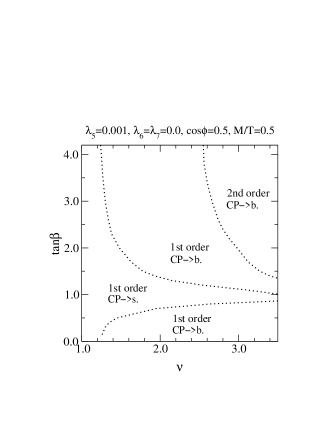
Figure 2: The 1-loop phase diagram for the transition from the C violating phase to the usual broken and symmetric phases as $y$ is varied, for fixed $\lambda_{5}=0.001,\lambda_{6}=\lambda_{7}=0$ ($\alpha_{6}=\alpha_{7}=\pi/2$), $\cos\phi=0.5$, $M/T=0.5$ ($m_{U}(T)/T=0.35$), $\hat{A}_{t}=\hat{\mu}=0$. The transition from the C violating phase can lead either directly to the symmetric phase (“s.”) or to the usual broken phase (“b.”), and it can be either of 1st or 2nd order.

We will also fix $\cos\phi=0.5$, which does not have a significant effect. Moreover, we choose here $\alpha_{6}=\pi/2$, $\alpha_{7}=\pi/2$, setting $\lambda_{6},\lambda_{7}$ to zero (according to Eqs. (C.24), (C.25), $\lambda_{6}=2\sqrt{\lambda_{1}\lambda_{5}}\cos\alpha_{6},\lambda_{7}=2\sqrt{\lambda_{2}\lambda_{5}}\cos\alpha_{7}$). If one would take other values, one needs to have an anti-correlation in the signs of $\lambda_{6},\lambda_{7}$, to get $M_{12}^{2}=m_{12}^{2}(T)+{\frac{1}{2}}\lambda_{6}v_{1}^{2}+{\frac{1}{2}}\lambda_{7}v_{2}^{2}$ close to zero; see Fig. 1. However, we again do not expect new qualitative effects from relaxing this assumption. As to the stop sector, we somewhat arbitrarily choose $m_{U}^{2}(T)/T^{2}\approx 0.13$, but vary $\hat{A}_{t},\hat{\mu}$ within $|\hat{A}_{t}|,|\hat{\mu}|\mathop{\raise 1.29167pt\hbox{$<$\kern-7.5pt\raise-4.73611pt\hbox{$\sim$}}}0.3$. We denote $M=\sqrt{2}m_{U}(T)/h_{t}$ (cf. Eq. (C.13)) so that $M/T=0.5$.

These choices fix the quartic couplings of the theory as well as the stop sector, but still leave the diagonal entries of the SU(2) scalar mass matrix, parameterised by $\nu,\tan\beta$ in Eqs. (C.10), (C.11), open. The perturbative phase diagram in this space, based on the full 1-loop effective potential in Eq. (4.2), is shown in Fig. 2. We have chosen a number of points from this diagram for further non-perturbative study, such that all different qualitative types of transitions are represented.

            

            

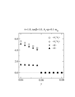
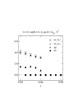
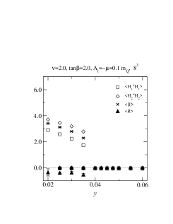
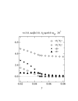
Figure 3: Top: Mean field estimates for the $y$-dependence of different expectation values, corresponding to the physical volume obtained with $\beta_{w}=8$, $N_{1}N_{2}N_{3}=20^{3}$. For $I$ the absolute value of the volume average is taken. Bottom: Lattice results at $\beta_{w}=8$. For the first two sets the transition is strongly of the first order, and a small volume has been used; in spite of this, some $y$-values allow for separate measurements in two different metastable phases. For the middle set, the transition goes on the lattice directly to the C conserving symmetric phase, rather than to the C conserving broken phase seen in the perturbative plot.

In Fig. 3, we show the mean field estimates for the behaviour of the operators in Eq. (3.3) for a few representative choices of parameters. These estimates follow from Eq. (3.8), with the 1-loop effective potential from Eq. (4.2), supplemented by a non-vanishing value of $\chi$ as needed in Eq. (3.8), whereby the contribution on the last line in Eq. (4.2) goes over into a sum over the eigenvalues of a 9$\times$9 matrix, with the radial $U$ direction coupled to the SU(2) scalars. (The Goldstone modes of $U$ appear separately as, e.g.,  in [17].)

The mean field estimates can be compared with the lattice results, shown also in Fig. 3 for the same parameter values. We observe that, as expected, the behaviours are quite close to each other. We then estimate that compared with Fig. 1, the largest value allowing for spontaneous C violation can change at most by

$$\delta\frac{m_{1}^{2}(T)+m_{2}^{2}(T)}{T^{2}}\approx 2\delta y_{c}\mathop{\raise 1.29167pt\hbox{$<$\kern-7.5pt\raise-4.73611pt\hbox{$\sim$}}}0.2,$$ (4.6)

where the upper bound is quite conservative.

4.4 Implications for the physical MSSM

Let us now compare Fig. 1 supplemented by Eq. (4.6), with the part of the parameter space allowed by the MSSM. One could make many comparisons, but we focus here on $m_{12}^{2}(T)/T^{2}$ and, in particular, $[m_{1}^{2}(T)+m_{2}^{2}(T)]/T^{2}$, cf. Eq. (4.4).

First of all, we recall from Fig. 1 that one needs small values of $M_{12}^{2}/T^{2}$ and therefore, due to the smallness of $\lambda_{6},\lambda_{7}$, small values of $m_{12}^{2}(T)/T^{2}$ (cf. Eq. (C.1)). It can be observed from Eq. (2.11) that in the MSSM this is easier to satisfy at finite temperatures than at zero temperature, due to a temperature correction which can cancel the $T=0$ part in $m_{12}^{2}(T)$ for $A_{t}\mu>0$. Furthermore, even if the experimental lower limit on $m_{A}$ appears to be rather high, $\sim 90$ GeV [10], one can at least partially compensate for this by taking a large $\tan\beta$, since only the combination $m_{A}^{2}\tan\beta/(1+\tan^{2}\beta)$ appears in Eq. (2.11).

However, the constraint on $[m_{1}^{2}(T)+m_{2}^{2}(T)]/T^{2}$ works in the opposite direction. To get spontaneous C violation $m_{1}^{2}(T)+m_{2}^{2}(T)$ should be small (Fig. 1), its order of magnitude given by $\lambda_{5}v^{2}$ (Eq. (4.4)). Finite temperature does not help with this constraint at all: $v^{2}$ gets smaller, while $m_{1}^{2}(T)+m_{2}^{2}(T)$ gets larger.

To be more precise, we obtain using Eqs. (2.9), (2.10) that in the MSSM,

$$m_{1}^{2}(T)+m_{2}^{2}(T)\approx m_{A}^{2}+0.5T^{2}+0.25T^{2}(1-|\hat{A}_{t}|^{2}-|\hat{\mu}|^{2}).$$ (4.7)

Let us now reiterate that in the limit of large $m_{Q}^{2}$ and small $m_{U}^{2}$ that we are working at, $1-|\hat{A}_{t}|^{2}-|\hat{\mu}|^{2}$ should in general be positive for the theory to be consistent from the point of view of boundedness and electroweak vacuum stability [49]. Taking into account also the experimental lower limit on the CP odd Higgs mass parameter $m_{A}\mathop{\raise 1.29167pt\hbox{$>$\kern-7.5pt\raise-4.73611pt\hbox{$\sim$}}}90$ GeV [10], we then get that in the MSSM,

$$[m_{1}^{2}(T)+m_{2}^{2}(T)]/T^{2}\mathop{\raise 1.29167pt\hbox{$>$\kern-7.5pt\raise-4.73611pt\hbox{$\sim$}}}1.3.$$ (4.8)

This holds for all temperatures below $100$ GeV, i.e., also in the broken electroweak Higgs phase.

This result can be contrasted with Fig. 1. We observe that there is no overlap, since $[m_{1}^{2}(T)+m_{2}^{2}(T)]/T^{2}\mathop{\raise 1.29167pt\hbox{$<$\kern-7.5pt\raise-4.73611pt\hbox{$\sim$}}}0.5$ always. A non-perturbative change of the order in Eq. (4.6) clearly cannot bridge the gap.

Figure 4: The tadpole graph leading to Eq. (4.10). The effective local quartic vertex shown, the second line in Eq. (2.1) with $\gamma_{i}$’s from Eq. (2.7), is a good approximation as long as $m_{U}^{2}\ll m_{Q}^{2}$.

It can be observed from Fig. 1 that increasing $m_{U}(T)$ seems to allow for larger values of $[m_{1}^{2}(T)+m_{2}^{2}(T)]/T^{2}$. However, this effect is not enough to change our conclusions. In fact, for large $m_{U}(T)$ the field $U$ can be integrated out, as we review in Appendix D, and the result is a theory of the form in Eq. (2.1) but without $U$. In this theory, there is an upper limit on $[m_{1}^{2}(T)+m_{2}^{2}(T)]/T^{2}$ leading to spontaneous C violation as well, numerically $[m_{1}^{2}(T)+m_{2}^{2}(T)]/T^{2}\mathop{\raise 1.29167pt\hbox{$<$\kern-7.5pt\raise-4.73611pt\hbox{$\sim$}}}0.4$ for $v/T\mathop{\raise 1.29167pt\hbox{$<$\kern-7.5pt\raise-4.73611pt\hbox{$\sim$}}}3.0$ [61]. The effect observed in Fig. 1 is equivalent to the fact seen in Eqs. (D.1), (D.2) that the effective $[m_{1}^{2}(T)+m_{2}^{2}(T)]/T^{2}$ after integrating out $U$ tends to decrease by increasing $m_{U}(T)$. More precisely, the last term in Eq. (4.7), $(h_{t}^{2}T^{2}/4)(1-|\hat{A}_{t}|^{2}-|\hat{\mu}|^{2})$, is multiplied by the factor

$$f=1-\frac{3}{\pi}\frac{m_{U}(T)}{T}.$$ (4.9)

However, this decrease does not continue forever, but the formula breaks down for large enough $m_{U}(T)$ when the high temperature expansion is no longer applicable, and $f$ then goes over into the tadpole integral shown in Fig. 4 (provided that still $m_{U}^{2}\ll m_{Q}^{2}$),

$$f\to\left.\frac{6}{\pi^{2}}\int_{0}^{\infty}dx\frac{x^{2}}{\sqrt{x^{2}+y^{2}}}\frac{1}{\exp({\sqrt{x^{2}+y^{2}}})-1}\right|_{y=m_{U}/T}.$$ (4.10)

This is always positive, so that $[m_{1}^{2}(T)+m_{2}^{2}(T)]/T^{2}$ does not decrease below $m_{A}^{2}/T^{2}+0.5\mathop{\raise 1.29167pt\hbox{$>$\kern-7.5pt\raise-4.73611pt\hbox{$\sim$}}}1.3$ even if $m_{U}(T)\mathop{\raise 1.29167pt\hbox{$>$\kern-7.5pt\raise-4.73611pt\hbox{$\sim$}}}T$, and our previous conclusion continues to hold.

In summary, spontaneous CP violation seems to be excluded in the MSSM both at $T=0$ and at finite temperatures around the electroweak phase transition.

4.5 Transitional CP violation

Let us finally come to the issue of “transitional CP violation”. There have been suggestions that even if not in the symmetric or broken phase, spontaneous C violation could take place within the phase boundary between the symmetric and broken phases [42, 43]. However, these suggestions could not be confirmed by later analyses for physical parameter values (particularly realistic $m_{A}$) [30]. Basically, the point is that as our discussion above indicated, spontaneous C violation is always more likely at large vevs, cf. Eqs. (C.2), (4.4). Thus it seems unlikely that C would be violated in the phase boundary, if it is not violated in the broken phase. Below, we will inspect the issue numerically at a physical phase boundary corresponding to the MSSM, and find the same conclusion. Let us note that, on the contrary, transitional C violation could take place in, say, the NMSSM [30, 29].

5 The strength of the physical phase transition

5.1 Parameter values

We now move to the electroweak phase transition in the physical MSSM. Let us start by choosing parameter values. We have previously carried out simulations corresponding to $\tan\beta=3,m_{H}=95$ GeV, a large $m_{A}\mathop{\raise 1.29167pt\hbox{$>$\kern-7.5pt\raise-4.73611pt\hbox{$\sim$}}}200$ GeV, and a light right-handed stop [19]. We found a transition which was somewhat stronger than in 2-loop perturbation theory and certainly strong enough for baryogenesis. Recently, 4d finite temperature lattice simulations have also been carried out in a scalar theory with MSSM type couplings, at $m_{H}\approx 45$ GeV [62]. There the transition is very strong, and it was found to agree well with perturbation theory.

We now want to take a larger $\tan\beta=12$ than in [19], corresponding to $m_{H}\approx 105$ GeV for a left-handed squark mass parameter $m_{Q}\approx 1$ TeV and a light right-handed stop. We also take a smaller $m_{A}\approx 120$ GeV for two reasons. First, because then the experimental Higgs mass lower bound is somewhat relaxed [10]. (Recently it has been suggested that the experimental Higgs mass lower bound may be further relaxed for such $m_{A}$ because of large explicit CP violation in the system, as we will have [63]–[66]). Second, because a smaller $m_{A}$ makes the heavy Higgs doublet eigendirection somewhat more dynamical, since effects related to it are suppressed by $\sim g_{w}^{2}T/(m_{A}^{2}+0.5T^{2})^{{\frac{1}{2}}}$, see Appendix A. This means that the situation could be favourable for “dynamical” CP violation [49] (i.e.,  a somewhat non-trivial profile for CP odd observables within the phase boundary, even if not actual spontaneous CP violation), as well as for having a non-trivial $\tan\beta$-profile [67, 20, 30], which might affect the actual baryon asymmetry produced [24]–[28].

We also introduce a non-vanishing squark mixing parameter $A_{t}\approx 200$ GeV, as well as gaugino and Higgsino mass parameters $M_{2}$, $\mu$, with $M_{2}\sim|\mu|\approx 200$ GeV. The strength of the phase transition depends little on these parameters [11]–[23]. In addition, to observe the CP violating effects more clearly, we choose a maximal explicit phase for the $\mu$-parameter, $\mu=i|\mu|$. The first and second generation squarks and sleptons are assumed heavy, whereby even such a large phase is not in conflict with electric dipole moment constraints [68]–[72].

Finally and most importantly, we take a negative right-handed squark mass parameter, $\tilde{m}_{U}^{2}\equiv-m_{U}^{2}>0$. Most of the time we work at $\tilde{m}_{U}=65$ GeV (see below). To summarise, we thus have

$$g_{w}^{2}\approx 0.42,\quad g_{s}^{2}\approx 1.1,\quad h_{t}\approx 1.0,$$ (5.1)

$$m_{Q}\approx 1\mbox{ TeV},\quad\tilde{m}_{U}\approx 65\mbox{ GeV},\quad m_{A}\approx 120\mbox{ GeV},\quad\tan\beta\approx 12,$$ (5.2)

$$A_{t}\approx|\mu|\approx M_{2}\approx 200\mbox{ GeV},\quad\mu\approx i|\mu|,$$ (5.3)

where on the first row the couplings are assumed to be evaluated at a scale $\sim 2\pi T$. These parameters correspond to a lightest physical Higgs mass of about 105 GeV, and a lightest stop mass of about 155 GeV, with an uncertainty of a few GeV.

Applying then the formulas in Appendix A.7 of [49] (and fixing $T\sim 95$ GeV, as suggested by 1-loop perturbation theory, inside logarithms and elsewhere where its effects are subdominant, in order to simplify the results), we obtain the following effective couplings for the theory in Eq. (2.1):

$$m_{1}^{2}(T)\approx 18380\mbox{ GeV}^{2}+0.1218T^{2},$$ (5.4)

$$m_{2}^{2}(T)\approx-3980\mbox{ GeV}^{2}+0.6218T^{2},$$ (5.5)

$$m_{12}^{2}(T)\approx(-1190-i100)\mbox{ GeV}^{2}+i0.0030T^{2},$$ (5.6)

$$m_{U}^{2}(T)\approx-4225\mbox{ GeV}^{2}+0.8534T^{2},$$ (5.7)

$$\gamma_{1}\approx-0.044,\quad\gamma_{2}\approx 0.96,\quad\gamma_{12}\approx-i0.037,\quad\lambda_{U}\approx 0.197,$$ (5.8)

$$\lambda_{1}\approx 0.0652,\quad\lambda_{2}\approx 0.1188,\quad\lambda_{3}\approx 0.0673,\quad\lambda_{4}\approx-0.1948,$$ (5.9)

$$\lambda_{5}\approx-0.00019,\quad\lambda_{6}\approx i0.0017,\quad\lambda_{7}\approx i0.0022.$$ (5.10)

We should stress that these numbers have of course some perturbative errors, but this is not essential for our main statements. Indeed, we will compare 3d perturbation theory with 3d lattice simulations, and precisely the same parameters in Eqs. (5.4)–(5.10) are chosen in both cases. This will allow us to unambiguously find out whether there are non-perturbative effects in the system. Such non-perturbative effects will then remain very similar even if the 4d parameter values are changed slightly, or if the reduction computation leading to Eqs. (5.4)–(5.10) is carried out more precisely.

Finally, let us mention a technical point. We treat the mass parameters in Eqs. (5.4)–(5.7) as those at the scale $\bar{\mu}=T$ inside the 3d theory (to be more precise: we choose the $\Lambda$-parameters discussed in Appendix A.4 to be $\Lambda\sim 1.0T$). In order to remove the ambiguity from this choice, a complete 2-loop dimensional reduction computation would be needed for the mass parameters [52]. Unfortunately, such computations have been carried out only in special cases. One is the Standard Model [52], where it turns out that numerically $\Lambda\sim 7T$. In [19] it was argued that this should be expected also for the MSSM. An explicit computation was then carried out in [21] for a small $m_{Q}\sim 300$ GeV, and the actual scale was found to be of order $\sim 2T$ for the diagonalized Higgs mass parameter (see Appendix A for the definition), $\sim 7T$ for the stop mass parameter. However, the scales depend on the other parameters of the theory. While the way to carry out the computation for large $m_{Q}$, the case relevant here, has also recently been clarified [73], explicit results for the full MSSM are still missing, so we cannot simply take over old values.

Fortunately, it turns out that this ambiguity is of very little significance for our results. Indeed, we have tested the effect of changing from $\Lambda\sim T$ to $\Lambda\sim 7T$ with 2-loop perturbation theory inside the 3d theory. We find that the critical temperature, as well as the value of $\tilde{m}_{U}$ corresponding to the “triple point” (see Fig. 5) change by a few GeV, but apart from this shift the values of $v/T$ at the transition remain almost the same. Thus the ambiguity is completely inconsequential, if we normalise our parameter values with respect to the triple point.

5.2 Phase transition in perturbation theory

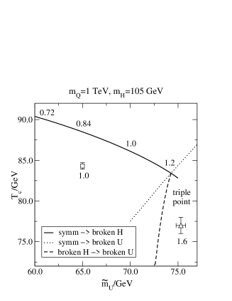
Figure 5: The perturbative 2-loop phase diagram for $m_{Q}=1$ TeV. The values of $v/T$ at the transition point are also shown. Lattice results are displayed at $\tilde{m}_{U}=65$ GeV (square), and at the triple point (triangle). The lattice triple point errorbars include only statistical errors (see the text), and are thus an underestimate.

         

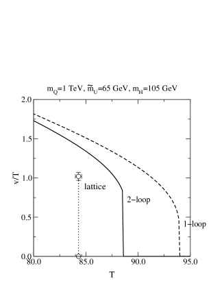
Figure 6: The properties of the phase transition in 1-loop and 2-loop perturbation theory, as well as on the lattice. Left: the perturbative effective potentials at the corresponding critical temperatures. Right: the vacuum expectation values as a function of $T$. The lattice value refers to $\left.v/T\right|_{\mbox{\scriptsize lattice}}=(2\Delta\sum_{i}\hat{H}_{i}^{\dagger}\hat{H}_{i})^{{\frac{1}{2}}}$, cf. Eqs. (3.1), (3.5).

For the parameter values in Eqs. (5.4)–(5.10), the theory in Eq. (2.1) has a first order electroweak phase transition. Let us first discuss its properties in perturbation theory. In the following, we use the Landau gauge and the scale parameter $\bar{\mu}=T$, as is conventional in the literature.

As we mentioned in Sec. 2.1, for studying the strength of the phase transition the theory in Eq. (2.1) can be simplified by integrating out a linear combination of the two Higgs doublets. This is not only a convenience but also a way of increasing the accuracy of perturbation theory: large effects related to a heavy excitation get resummed. We discuss the details of the integration out in Appendix A. After the integration out, we can directly employ the 2-loop effective potential computed in [19]. We may note that at 1-loop level we have also the effective potential in the full theory available, see Eq. (4.2), and in practice we find quite similar results as by using the diagonalized effective theory (to 1-loop accuracy).

In Fig. 5 we show the phase diagram as a function of $\tilde{m}_{U},T$. The three familiar types of transitions [17] are well visible. However, with our parameters, we observe that in fact a 2-stage transition as proposed in [17] is excluded, unlike with the parameter choice which we employed in [19]. Instead one has to worry about whether the metastability of the broken Higgs phase is sufficiently strong [74], if $\tilde{m}_{U}$ is very close to the triple point. However, we can here apply the logic of [22] in the opposite direction, and state that one would never tunnel into the broken $U$ direction even if possible in principle. (In the case of [22], the dashed line in Fig. 5 was tilted in the other direction, and the statement was that if one ends up in the phase with broken $U$, one can never get from there to the usual electroweak phase, even if that would be the thermodynamically stable phase.) Still, values $\tilde{m}_{U}\mathop{\raise 1.29167pt\hbox{$<$\kern-7.5pt\raise-4.73611pt\hbox{$\sim$}}}70$ GeV would seem safest. We choose here $\tilde{m}_{U}=65$ GeV for further study.

As discussed in Sec. 3.3, the strength of the phase transition is in perturbation theory usually addressed in terms of $v/T$ rather than $H_{1}^{\dagger}H_{1}+H_{2}^{\dagger}H_{2}$, or $h^{\dagger}h$ in the diagonalized theory of Appendix A. The relation is then obtained from Eq. (3.4) or, if one converts from lattice to perturbation theory, from Eq. (3.5). We show the 1-loop and 2-loop results for $v/T$ in Fig. 6. We observe the familiar feature that the transition is significantly stronger at 2-loop level [13]–[21], which is related to the fact that the critical temperature $T_{c}$ is lower.

Finally, let us recall that because a certain combination of the Higgs doublets is heavy, the transition takes essentially place in one “light” direction in the field space much like in the Standard Model (see also Fig. 14 below), and the sphaleron energy is really determined by the value of $H_{1}^{\dagger}H_{1}+H_{2}^{\dagger}H_{2}$ in the broken phase. Note, in particular, that even though possible in principle [75], we would not expect the sphaleron bounds to be modified by the CP violation apparent in the couplings in Eqs. (5.4)–(5.10), because the Higgs direction orthogonal to the light eigenmode $h$ is indeed so heavy that effects related to it are strongly suppressed; see Appendix A.

5.3 Lattice simulations

$\beta_{w}$ volumes 8 $12^{3}$    $16^{3}$    $24^{3}$ 12 $16^{3}$    $24^{3}$    $32^{3}$ 16 $24^{3}$    $32^{3}$ 24 $32^{3}$    $40^{3}$    $56^{3}$

Table 1: Lattice spacings $\beta_{w}=4/(g_{w}^{2}aT)$ and lattice volumes, used for simulations at the transition temperature. All the simulations here are multicanonical.

In order to inspect the reliability of the perturbative estimates discussed above, we have carried out lattice simulations at $\tilde{m}_{U}=65$ GeV. First, a series of simulations was performed in order to determine the transition temperature $T_{c}$, the value of $v/T$ in the broken phase, the latent heat and the surface tension. The lattice sizes and lattice spacings are shown in Table 1. For each lattice listed we performed 50 000 – 360 000 compound iterations (5 $\times$ overrelaxation + 1 $\times$ heat bath). All of the simulations in Table 1 are multicanonical, i.e. the probability distribution has been modified to enhance the tunnelling between the broken and symmetric phases. For technical details, we refer to Sec. 3.2 and to ref. [19], which includes a detailed description of the application of the multicanonical method to the MSSM (albeit with only one SU(2) Higgs doublet).

At this point in parameter space the transition is relatively strong, as can be seen from the probability distributions of $H_{1}^{\dagger}H_{1}+H_{2}^{\dagger}H_{2}$ in Fig. 7. The distributions measured have here been reweighted to a temperature which gives equal probabilistic weights to the symmetric and broken phases (“equal weight histograms”).

Figure 7: The “equal weight” probability distributions of $(H_{1}^{\dagger}H_{1}+H_{2}^{\dagger}H_{2})/T^{2}$ (without the subtractions in Eq. (B.7)), measured from $\beta_{w}\equiv 4/(g_{w}^{2}aT)=12$ lattices.

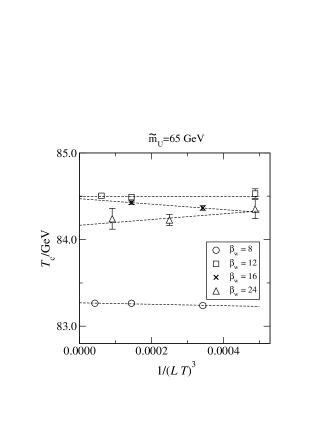
Figure 8: The transition temperatures at different $\beta_{w}$’s and volumes, plotted against inverse volume. The transition temperatures have been determined with the “equal weight” criterion.

5.4 Results for various physical observables

Critical temperature:

Tuning the temperature so that the “order parameter” probability distributions have equal weights in symmetric and broken phases (see Fig. 7) gives a good definition for the transition temperature at finite volumes. We use this definition in what follows. Other definitions can be found in [19]; at the infinite volume limit all of these give identical results within statistical errors.

In Fig. 8 the equal weight temperatures are shown for all lattices in Table 1. For each lattice spacing we perform an infinite volume extrapolation linear in $1/(\mbox{volume})$. As seen in Fig. 8, the slopes of the fits appear to behave somewhat unsystematically. This is caused by the statistical errors of the individual measurements: the differences of the transition temperatures at different volumes are small enough that a constant (in $1/V$) fit at each of the lattice spacings could have been used.

On the other hand, we note a clear lattice spacing dependence between $\beta_{w}=8$ and the other sets of data. Obviously here the lattice spacing $a=4/(\beta_{w}g_{w}^{2}T)\approx 1.2/T$ is so large that the subleading corrections start to be significant. Thus, we use only the infinite volume extrapolations at $\beta_{w}=12$, 16 and 24 to estimate the continuum limit value, with the result

$$T_{c}=84.3\pm 0.3\,\mbox{GeV}.$$ (5.11)

This can be compared with the 2-loop perturbative value 88.5 GeV (see Figs. 5, 6). Indeed, the difference between the perturbative and the non-perturbative results is much larger than the difference between the results from different lattice spacings. This behaviour agrees qualitatively with our previous study [19].

Figure 9: The joint probability distribution of $\hat{H}_{1}^{\dagger}\hat{H}_{1}+\hat{H}_{2}^{\dagger}\hat{H}_{2}$ and $\hat{U}^{\dagger}\hat{U}$ at the triple point, measured from a $\beta_{w}=12$, $12^{3}$ lattice. The transition symmetric$\leftrightarrow$broken $U$ is weak, as can be seen from the small suppression between the peaks. This means that it is relatively easy to end up in the phase with broken $U$, if one goes too close to the triple point. On the other hand, there is a suppression of $\sim e^{-20}$ between the symmetric and broken $H$ peaks, signalling a strong transition.

Triple point:

In the perturbative phase diagram in Fig. 5, there is a “triple point” at $\tilde{m}_{U}\approx 74.3$ GeV, $T_{c}\approx 83.4$ GeV, with $v/T\approx 1.24$. We have determined the triple point location also with lattice simulations at small volumes, using $\beta_{w}=12$, volume $12^{3}$ (see Fig. 9), and $\beta_{w}=16$, volume $16^{3}$. It is technically difficult and very time-consuming to perform multicanonical simulations at the triple point, and we did not attempt to do an infinite volume extrapolation here. However, the results obtained from the two lattices agree reasonably well with each other, and we can make an estimate for the triple point location, $T_{\rm triple}\approx 77\pm 1$ GeV, $\tilde{m}_{U,\rm triple}\approx 75.3\pm 0.5$ GeV, with an expectation value (see below for its determination) $v/T\approx 1.65\pm 0.10$. We emphasize that these values are just rough estimates; the lack of an infinite volume extrapolation can be significant here, since the SU(3) $U$-field is very light at this point. Nevertheless, a comparison with the perturbative values is shown in Fig. 5. The deviation from the perturbative triple point matches the behaviour at $\tilde{m}_{U}=65$ GeV, where we have a much better control of the systematics.

Order parameter discontinuities:

Going back to $\tilde{m}_{U}=65$ GeV, the discontinuity $\Delta v/T=[2\sum_{i}\Delta H_{i}^{\dagger}H_{i}/T^{2}]^{1/2}$ can be quite precisely measured from the probability distributions (Fig. 7), by determining the positions of the symmetric and broken phase peaks separately. The results for all the volumes are shown in the left panel of Fig. 10. We see that for each lattice spacing, $v/T$ remains practically constant over the whole range of volumes. Nevertheless, we again make an extrapolation linear in $1/V$ to the infinite volume limit.

           

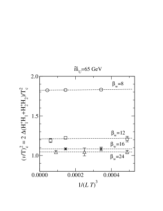
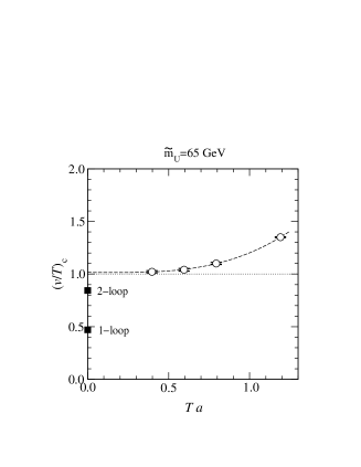
Figure 10: Left: the finite volume dependence of $(v/T)_{c}^{2}$, together with infinite volume extrapolations. Right: the continuum extrapolation of $(v/T)_{c}$. Note that in units of $T^{-1}$, we are able to operate on relatively large lattice spacings $a$, since the most ultraviolet fluctuations of the original 4d theory have been removed by dimensional reduction.

The lattice spacing dependence is relatively pronounced, and the discontinuity $\Delta v$ becomes smaller as the continuum limit is approached. In the right panel of Fig. 10 we show the infinite volume extrapolations of $v/T$ against the lattice spacing. The data is extrapolated to the continuum limit using a polynomial fit of the form $c_{0}+c_{2}(aT)^{2}+c_{3}(aT)^{3}$. A priori, there is no reason why a term linear in $a$ should not be there; however, when it is included in the fits, $v/T$ invariably becomes larger as $a$ is decreased at small $a$. While in principle possible, this kind of a behaviour does not seem very plausible, especially in view of the fast apparent convergence of the data as $a$ is decreased in Fig. 10. Thus, we effectively force the term linear in $aT$ to be $\geq 0$ in the extrapolation. This behaviour persists if we drop the largest lattice spacing $aT=1.2$ from the analysis; in this case we obtain a good fit with the ansatz $c_{0}+c_{2}(aT)^{2}$, with almost the same value and errors for $c_{0}$. Thus, in the continuum limit, we quote our result as

$$(v/T)_{c}=1.02\pm 0.05\,,$$ (5.12)

where the error includes both the statistical errors and the ambiguity due to different extrapolations. This can be compared with the 1-loop perturbative result $(v/T)_{c}\approx 0.47$, and the 2-loop perturbative result $(v/T)_{c}\approx 0.85$. See Figs. 6, 10 for comparisons.

In addition to the discontinuities at the transition point, we have also determined the Higgs condensates at temperatures close to $T_{c}$. In the first panel of Fig. 12 we show how the bilinears $H_{2}^{\dagger}H_{2}$, $R=\mathop{\rm Re}H_{1}^{\dagger}\tilde{H}_{2}$, $I=\mathop{\rm Im}H_{1}^{\dagger}\tilde{H}_{2}$ behave as we go through the transition. Since in our simulations $\tan\beta=12$ is large, $H_{1}^{\dagger}H_{1}$ is practically constant on the scale of the plot. We note that $I$ remains almost constant, too, and has at most only a very small jump at the transition; it is non-zero overall because of the small imaginary parts in the effective parameters, particularly $m_{12}^{2}(T)$, in Eqs. (5.4)–(5.10).

Latent heat:

The latent heat of the transition is closely related to the order parameter discontinuities of the 3d theory. In general, the latent heat is determined by

$$L=-T_{c}\bigg{(}{\frac{d(\Delta f)}{dT}}\bigg{)}_{T=T_{c}}\,,$$ (5.13)

where $\Delta f=f_{\mbox{\scriptsize symmetric}}-f_{\mbox{\scriptsize broken}}$ is the free energy density difference between the symmetric and broken phases, and the derivative is to be taken along the metastable branches. More concretely, $L$ measures the discontinuity in the energy density.

In our 3d theory with the parametrization in Eqs. (5.4)–(5.10), explicit temperature dependence appears only in the Higgs mass parameters. Thus, following [53, 55], the latent heat becomes

$$L=T_{c}^{3}\Delta\left\langle U^{\dagger}U{\frac{d}{dT}}{\frac{m_{U}^{2}(T)}{T^{2}}}+\sum_{i=1}^{2}H_{i}^{\dagger}H_{i}{\frac{d}{dT}}{\frac{m_{i}^{2}(T)}{T^{2}}}+\bigg{(}H_{1}^{\dagger}\tilde{H}_{2}{\frac{d}{dT}}{\frac{m_{12}^{2}(T)}{T^{2}}}+\mbox{H.c.}\bigg{)}\right\rangle,$$ (5.14)

where $\Delta\langle\cdot\rangle=\langle\cdot\rangle_{\rm broken}-\langle\cdot\rangle_{\rm symmetric}$.

We observe that the latent heat behaves numerically very much like the discontinuity in $v/T$, but with slightly larger statistical errors, since more condensates are involved. We do not show a separate figure. It should be noted that the $U^{\dagger}U$-term in Eq. (5.14) is significant, despite the fact that the $U$-field remains “unbroken” at all temperatures at this $\tilde{m}_{U}$. This is because $\langle U^{\dagger}U\rangle$ is somewhat smaller in the phase where the SU(2) Higgs fields $H_{i}$ are “broken”.

We use similar infinite volume and continuum extrapolations for the latent heat as for the condensate $v/T$ in Fig. 10. The final result (at our specific parameter point) becomes

$$L/T_{c}^{4}=0.42\pm 0.03\,,$$ (5.15)

which is substantially larger than the perturbative 2-loop value $L/T_{c}^{4}\approx 0.26$. The difference is quite large, but it is again qualitatively similar to the one observed in [19].

            

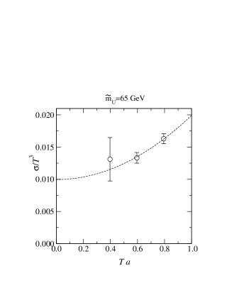
Figure 11: Left: the finite volume dependence of the surface tension. Right: a continuum estimate. We should stress that our determination of $\sigma/T_{c}^{3}$ is not meant to be nearly as precise as the determination of $(v/T)_{c}$ (see the text).

Surface tension:

We measure the tension of the interface between the symmetric and broken phases (also called the phase boundary) with the histogram method. The surface tension $\sigma$ equals the additional free energy/area carried by the interface. This extra free energy suppresses mixed phase configurations by a factor $\propto\exp(-\sigma A/T)$, where $A$ is the area of the interfaces. This causes a characteristic “valley” between the symmetric and broken phase peaks in probability distributions of order parameter like quantities; see, for example, Fig. 7.

In the histogram method one uses the mixed phase suppression to measure the surface tension. Assuming that the interfaces are perpendicular to the $x_{3}$-axis direction, $\sigma$ can be obtained from

$${\frac{1}{2L_{1}L_{2}}}\ln{\frac{P_{\rm max}}{P_{\rm min}}}\rightarrow{\frac{\sigma}{T}}\mbox{~{}~{}~{}~{}~{}~{}~{} as ~{}}V\rightarrow\infty\,.$$ (5.16)

Here $P_{\rm max,min}$ are the maximum and minimum of the peaks of the probability distribution, and $L_{i}=N_{i}a$ are lattice extensions in physical units. The factor $2$ appears in front of $L_{1}L_{2}$, because there are two interfaces in a box with periodic boundary conditions.

In the actual analysis we measure $\sigma$ from histograms of $H_{1}^{\dagger}H_{1}+H_{2}^{\dagger}H_{2}$. These are reweighted to a temperature where the peak heights are equal, which simplifies the analysis. We also use a finite volume scaling ansatz similar to our earlier work [19],

$${\frac{\sigma}{T_{c}^{3}}}={\frac{1}{2(LT)^{2}}}\left[\ln{\frac{P_{\rm max}}{P_{\rm min}}}+{\frac{1}{2}}\ln LT+\mbox{const.}\right],$$ (5.17)

where we have employed the fact that our lattices are all cubic, $L_{1}=L_{2}=L_{3}=L$.

In Fig. 11 we show the rough infinite volume extrapolations of $\sigma/T_{c}^{3}$ from $\beta_{w}=12$, 16 and 24 lattices. (For this observable, $\beta_{w}=8$ gives a surface tension larger by about a factor of 5, and we do not include it in the analysis.) The continuum limit estimate of $\sigma$ becomes now

$$\sigma/T_{c}^{3}\approx 0.010\pm 0.05.$$ (5.18)

The 2-loop perturbative value is $\sigma/T_{c}^{3}\approx 0.017$, which is larger than the lattice value. However, we stress first of all that our lattice determination is quite rough here, as we have only used cubic volumes, not the cylindrical ones often employed for getting good infinite volume extrapolations (see, e.g., [19]). Second, we should also remember that in the perturbative estimate no account is taken of the effects related to derivative terms discussed in [76, 77, 78, 79, 35], which would decrease that value. Nevertheless, the situation is certainly different from the case studied in [19] where even the raw perturbative value was smaller than the lattice value. On the other hand, the situation is qualitatively similar to the case of the Standard Model [55], where the transition is of a relatively weak strength compared with [19], as it is here too.

Correlation lengths:

   

   

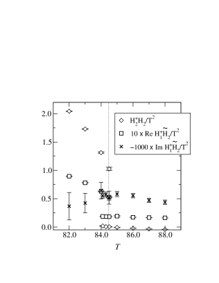
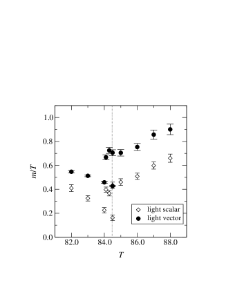
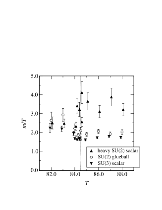
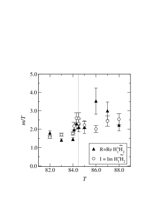
Figure 12: Top left: Higgs bilinears, subtracted according to Eq. (B.7), across the transition at $\beta_{w}=16$, volume $=32^{3}$. The vertical dotted line shows the location of $T_{c}$. Top right: light SU(2) scalar and vector inverse correlation lengths, $m/T$. Bottom left: heavy SU(2) scalar, SU(2) glueball and SU(3) scalar inverse correlation lengths. Bottom right: inverse correlation lengths related to the operators $R,I$. All the numbers in the bottom panels have relatively large systematic errors (see the text), and could almost be compatible with each other.

Next, let us explore spatial correlation lengths around the transition temperature. As usual, their inverses are called “screening masses”. The masses are measured from the 0-momentum correlation functions

$$C_{a}(x_{3})=\sum_{{\bf x},{\bf y}}\langle O_{a}({\bf y},0)O_{a}({\bf x},x_{3})\rangle\propto\exp[-m_{a}x_{3}],$$ (5.19)

where ${\bf x},{\bf y}$ are in the transverse $(x_{1},x_{2})$-plane, and the gauge invariant operator $O_{a}(x)$ is one of the following:

$$\begin{array}[]{ll}\mbox{C even SU(2) scalars:}&S^{w}_{a}(x)=H_{a}^{\dagger}(x)H_{a}(x),~{}~{}R(x)=\mathop{\rm Re}H_{1}^{\dagger}(x)\tilde{H}_{2}(x),\\ \mbox{C odd SU(2) scalar:}&I(x)=\mathop{\rm Im}H_{1}^{\dagger}(x)\tilde{H}_{2}(x),\\ \mbox{SU(2) vectors:}&V^{w}_{a,i}(x)=\mathop{\rm Im}H_{a}^{\dagger}(x)U^{w}_{i}(x)H_{a}(x+\hat{i}),\\ \mbox{SU(2) $O^{++}$ glueballs:}&G^{w}(x)=1-{\frac{1}{2}}{\rm Tr\,}P_{12}^{w}(x),\\ \mbox{SU(3) scalar:}&S^{s}(x)=U^{\dagger}(x)U(x),\\ \mbox{SU(3) vector:}&V^{s}_{i}(x)=\mathop{\rm Im}U^{\dagger}(x)U^{s}_{i}(x)U(x+\hat{i}),\\ \mbox{SU(3) $O^{++}$ glueballs:}&G^{s}(x)=1-{\frac{1}{3}}\mathop{\rm Re}{\rm Tr\,}P_{12}^{s}(x).\\ \end{array}$$

Here $i=1,2$; $a=1,2$ labels the two SU(2) Higgs fields; $U_{i}^{w}$ and $U_{i}^{s}$ are the standard lattice SU(2) and SU(3) gauge links (denoted by $U^{w}_{{{\bf x}},i},U^{s}_{{{\bf x}},i}$ in Eq. (3.1)); and $P^{w}_{12},P^{s}_{12}$ are $(x_{1},x_{2})$-plane plaquettes constructed from these links. In order to reduce statistical noise, we use recursive blocking and smearing of the gauge and Higgs fields along $(x_{1},x_{2})$-planes, and construct operators and measure all of the correlation functions from the blocked fields at each blocking level. The blocking is repeated up to 4 times. For details of the recursive blocking procedure we employ here, we refer to [19] (see also [80]).

The measurement of the correlation lengths in an interacting theory is complicated by the fact that all the operators in a given quantum number channel in general couple to the same set of physical states. For example, we can expect that all of the scalar operators above, including the $O^{++}$ glueballs, will in the limit $x_{3}\rightarrow\infty$ yield the screening mass of the lightest scalar state. On the other hand, in the real world the correlations may behave at intermediate distances in a different way, and to fully resolve this behaviour one usually measures the cross-correlation matrix of a large set of operators in a given quantum number channel, and diagonalises it.

However, in our case when only rough qualitative accuracy is needed, it turns out that this is not necessary: since we use a large $\tan\beta=12$, the active Higgs component in the transition projects almost completely to $H_{2}$, and correspondingly the light scalar and vector states couple strongly only to the operators $S_{2}^{w}$ and $V_{2,i}^{w}$, respectively. Moreover, the “coupling” (or overlap) of the SU(2) pure gauge and the whole SU(3) sector to the SU(2) scalar Higgs sector is weak. All in all, this implies that we can obtain the heavier scalar and vector screening masses just by measuring the exponential fall-offs of the corresponding correlation functions at intermediate distances; the accuracy of this approach is quite sufficient for our conclusions.

On the second panel of Fig. 12 we show the light SU(2) scalar and vector masses, and on the third and fourth panel the heavier masses. The lightest mass scale at the transition is an order of magnitude smaller than the heavy scales. This makes the condition in Eq. (3.2) very difficult to meet in practice, and in our case the first part $a\ll\xi_{\mbox{\scriptsize min}}$ is barely true. This circumstance also makes the measurement of the heavy masses difficult, since the correlation functions vanish into noise after a few lattice units, which explains the large errors in the data. However, for our purposes the accuracy obtained is sufficient.

We may now note first of all that while the large mass scales make the extrapolation to the continuum limit delicate (necessitating several lattice spacings, as we have), experience from QCD [81] indicates that the mass scales $\mathop{\raise 1.29167pt\hbox{$<$\kern-7.5pt\raise-4.73611pt\hbox{$\sim$}}}3T$ are still far from being too large for us to have any concerns about the applicability of dimensional reduction, used in the construction of the 3d effective field theory. The integration out of the Matsubara zero modes of the temporal components of the gauge fields is clearly more critical, but as we have discussed in [49], we expect even that to be reasonably under control. In any case, those masses are still much above the lightest ones in the system ($\ll T$), which determine the non-perturbative thermodynamical properties of the transition.

Furthermore, the screening mass spectra measured add further confidence to two statements we have made on other grounds before: (1) The correlation length related to $I$ is short, and thus not at all “critical”. This means that we are far from the possibility of spontaneous C violation. (2) The heavy SU(2) scalar correlation length is much shorter than the light one, and thus again far from “critical”. This means that it is only the “light” combination of the two Higgs doublets which is really “dynamical” at the transition point, and any effects related to the other one are suppressed.

6 The properties of the physical phase boundary

We now turn to the study of the properties of the phase boundary. We have outlined the measurements to be carried out, as well as some caveats in them, in [49].

In order to study a phase boundary, we have to make sure that there really is one on the lattice. This can be achieved by restricting, say, the volume average of $h^{2}\equiv H_{1}^{\dagger}H_{1}+H_{2}^{\dagger}H_{2}$ to a narrow band around $(h^{2}_{\rm symmetric}+h^{2}_{\rm broken})/2$. Provided that the volume of the system is large enough, this guarantees that the system will always remain in a broken + symmetric mixed state, with corresponding phase boundaries, or interfaces.

In the case at hand the interfaces are rather thick, and because of the periodic boundary conditions, there will be two interfaces spanning the lattice. This makes it advantageous to use cylindrical lattices: because of the surface tension, the interfaces will be preferentially oriented along the smallest cross-sectional area across the lattice, making them well separated along the longest lattice direction ($x_{3}$, say). This has the further advantage that we always know the orientation of the interfaces. Our interface simulations were made on $\beta_{w}=8$, $12^{2}\times 96$, and $\beta_{w}=16$, $24^{2}\times 192$ lattices, using up to 450 000 compound update sweeps per lattice.

6.1 Observables

We study the interface properties by looking at the Higgs bilinear operators in Eq. (3.3) as follows: first, for each configuration, we average the bilinears across the $(x_{1},x_{2})$-plane, so that we obtain them as functions of the $x_{3}$-coordinate. Then we average over all configurations in two ways: (1) the bilinears are measured as functions of the distance from a certain reference point, and (2) one bilinear is measured as a function of another. Let us look at these cases separately.

(1) Interface profiles:

The Monte Carlo simulation method described does not specify the location of the interfaces along the $x_{3}$-direction. However, in order to measure the profiles of various observables across the interface, we have to find a reference point in the $x_{3}$-direction, configuration by configuration (i.e., we have to remove the zero mode). Some care has to be taken here: for example, one may locate the $x_{3}$-value where $h^{2}$, averaged over $x_{1}$ and $x_{2}$, reaches the value half-way between the symmetric and broken phase ones. However, since $h^{2}$ (as any other local quantity) has large fluctuations, this kind of a sharply defined location will cause the configuration to be shifted such that the natural fluctuations across the interface may be summed “in phase”, which tends to distort the profile. The problem can be avoided by using a “softer” filter function. In this work employ the fact that there are two interfaces on a periodic lattice: thus we can find the “symmetry point” $x_{3,0}$ of the profile by taking a Fourier transform ($N_{3}$ is the extent of the lattice in the direction of $x_{3}$),

$$C=\sum_{x_{3}}h^{2}(x_{3})e^{i2\pi x_{3}/N_{3}}\equiv A\,e^{i2\pi x_{3,0}/N_{3}}.$$ (6.1)

Thus $x_{3,0}=N_{3}/(2\pi)\times(\mbox{polar angle of $C$})$. Configurations are then superimposed around this point.

In Fig. 13 we plot the profiles of the bilinears $H_{1}^{\dagger}H_{1}$, $H_{2}^{\dagger}H_{2}$, $R=\mathop{\rm Re}H_{1}^{\dagger}\tilde{H}_{2}$ and $I=\mathop{\rm Im}H_{1}^{\dagger}\tilde{H}_{2}$, measured from the $\beta_{w}=16$ lattice. (We observe no qualitative change compared with the $\beta_{w}=8$ lattice.) Only half of the profiles (one interface) are shown. Besides the obvious one in magnitudes, it is difficult to see qualitative differences between $H_{1}^{\dagger}H_{1}$, $H_{2}^{\dagger}H_{2}$ and $R$ across the interface.

Figure 13: The profiles of the operators in Eq. (3.3) as a function of the spatial coordinate across the wall. The cross-sectional area here is $\sim(14/T)^{2}$. The subtraction in Eq. (B.7) has not been carried out.

As for the C odd condensate $I$, its magnitude is even smaller and the errorbars correspondingly larger. For clarity, we have smoothed $I(x_{3})$ in Fig. 13 by an approximate Gaussian smearing:

$$I(x_{3})\leftarrow{\frac{1}{3}}[I(x_{3}-a)+I(x_{3})+I(x_{3}+a)]\,,$$ (6.2)

and repeated 4 times. Without this additional smearing it would be difficult to see any structure in the plot. After the smearing, we observe that $I$ increases slightly when the broken phase is entered. The overall negative value of $I$ is due to the small imaginary part of the $m_{12}^{2}(T)$ parameter, Eq. (5.6) (see Appendix A.1).

From Fig. 13 we see that the interface is rather thick: if we fit $H_{i}^{\dagger}H_{i}$ to a function of the form $a+b\tanh((x_{3}-c)/L)$, we obtain $L\sim 9/T$. However, one should bear in mind that in 3 dimensions the apparent interface thickness suffers from a logarithmic divergence as the area is increased (see, e.g., [82]). A natural way to resolve this arbitrariness is to consider the interfaces on physically relevant length scales. For our case, the longest correlation length $\xi_{\mbox{\scriptsize max}}$ at the transition is $\sim 6/T$ (see Fig. 12), so that the interfaces in Fig. 13 correspond to a cross-sectional area $\sim(2\xi_{\mbox{\scriptsize max}})^{2}$ .

(2) $H_{1}^{\dagger}H_{1}$ vs. $H_{2}^{\dagger}H_{2}$ and $I$ vs.  $R$ across the interface:

Instead of plotting the bilinears as functions of $x_{3}$, it can be more illustrative to consider the behaviour of one condensate as a function of another. This way there is no logarithmic divergence visible, and no need to locate the interface on the lattice.

         

Figure 14: Behaviour of (unsubtracted) $H_{2}^{\dagger}H_{2}$, plotted against $H_{1}^{\dagger}H_{1}$, and $-I=-\mathop{\rm Im}H_{1}^{\dagger}\tilde{H}_{2}$, plotted against $R=\mathop{\rm Re}H_{1}^{\dagger}\tilde{H}_{2}$, across the interface. Values are in units of $T^{2}$. The dashed curve on the left is a straight line, and solid curves are fits.

         

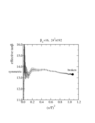
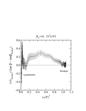
Figure 15: Left: behaviour of the effective $\tan\beta$, Eq. (3.5), across the interface. We note that the “dynamical” value differs only a little from the zero temperature input value $\tan\beta\approx 12.0$. Nevertheless, the effective $\tan\beta$ is not constant across the interface, but varies by a relative amount $\mathop{\raise 1.29167pt\hbox{$<$\kern-7.5pt\raise-4.73611pt\hbox{$\sim$}}}5$%. Right: the same data, plotted as $(v/v_{\mbox{\scriptsize broken}})(\tan\beta-\tan\beta_{\mbox{\scriptsize broken}})$.

In Fig. 14 we show $H_{2}^{\dagger}H_{2}$ as a function of $H_{1}^{\dagger}H_{1}$, and $I$ as a function of $R$. In the former case, there is a small but statistically clear deviation from the straight line between the symmetric and broken phases. We show the same data in Fig. 15 using the definition in Eq. (3.5).

We observe that in terms of $v_{i}=\sqrt{2\Delta H_{i}^{\dagger}H_{i}}$, the deviation from a straight line is ${\cal O}(\mbox{a few }\times 10^{-2})$. We also observe that C violation has some structure: the operator $I$ tends to saturate close to the broken phase value considerably faster than R (or $v/T$). However, we do not observe any significant amplification of $I$ inside the interface, and thus no sign of transitional C violation.

The orders of magnitude observed for the variation in $I$ and $\tan\beta$ agree roughly with perturbation theory [67, 20, 30] and, in the case of $\tan\beta$, with previous 4d simulations [62], although in most cases the parameter values were not identical to ours.

7 Summary and Conclusions

         

         

Figure 16: The Higgs mass $m_{H}$ and broken phase expectation value $v/T$ at the triple point (see Fig. 5) according to 2-loop perturbation theory, as a function of various quantities. The vertical lines indicate the location of our reference parameter values. The Higgs mass is computed with the 1-loop relations specified in [49] (corresponding to [84]). Note that the combination relevant for large $m_{A}$, $A_{t}-\mu^{*}\cot\beta$, is in most cases close to $A_{t}$, since we keep $\mu=i\,200$ GeV fixed and $\cot\beta=1/\tan\beta$ is small. In the values of $m_{H}$ we expect an uncertainty of a few GeV, due to unimplemented 2-loop zero temperature Higgs mass corrections, 2-loop dimensional reduction corrections, and perhaps also the fact that explicit CP violation has not been rigorously treated in the zero temperature relations we employ here [49] (for recent discussions, see [63]–[66]).

In this paper, we have studied the electroweak phase transition in the MSSM, with particular attention on CP violation in the background (“vacuum”) configuration, as well as on the strength of the phase transition.

The method we have used is based on 3d effective field theories, and their non-perturbative study. At finite temperatures around the electroweak phase transition, the thermodynamics of the MSSM can be represented by a theory containing two SU(2) Higgs doublets and one SU(3) stop triplet. Despite its complexity, we have demonstrated that this theory can be studied in a controlled way with lattice simulations.

The phase diagram of this theory is non-trivial, involving a phase where CP is (even) spontaneously violated, as well as a phase where the U(1) symmetry corresponding to a massless photon is broken. We have studied the phase with spontaneous CP violation in some detail. We have found that for the parameter values allowed by the MSSM, one does not end up in this phase close to the electroweak phase transition. In more general two Higgs doublet theories this could happen, with potential implications for baryogenesis.

We have then studied the electroweak phase transition at physical parameter values, in particular $m_{H}\approx 105$ GeV, not ruled out for the MSSM. We observe very clearly the feature familiar from our previous MSSM study [19] that the transition is significantly stronger than in 1-loop perturbation theory, and even stronger than at 2-loop level, due to the fact that the critical temperature $T_{c}$ is lower. Let us note that the situation is different from that studied with 4d simulations in [62], where the transition was quite strong ($m_{H}\approx 45$ GeV), and good agreement even with 1-loop perturbation theory was found. We do not consider there to be any discrepancy, however, since all our previous experience is that perturbation theory works the better, the smaller the Higgs mass.

At the point of our present study, we observe (Fig. 10) that the transition is strong enough for baryogenesis, since $v/T\approx 1.0$. (Based on analytic estimates, one would expect that $v/T$ has to be somewhat larger than 1.0 [55], but a dynamical lattice computation suggests that 1.0 should be enough [83]). However, this concerns a particular parameter point, and it is important to ask how much room there is around it.

To get a comprehensive estimate, let us now go to the point of the strongest possible transition, i.e. the triple point shown in Fig. 5. We then vary various parameters and use 2-loop perturbation theory to compute $v/T$. The results are shown in Fig. 16. We find the rather remarkable fact that the results are almost independent of the Higgs sector parameters $m_{A},\tan\beta$. This is so because at the triple point the properties of the transition are dictated by the stop sector.

On the other hand, the transition weakens rapidly away from the triple point (see Fig. 5). Our lattice results provide a strengthening effect which can partly compensate for this. Nevertheless, one needs to remain close to the triple point in any case, for instance $\tilde{m}_{U}\sim 65...77$ GeV for the parameters employed in Fig. 5. The perturbative range would have been $\tilde{m}_{U}\sim 69...74$ GeV.

Apart from $v/T$, we have also measured other important characteristics of the phase transition. The values of the latent heat $L/T_{c}^{4}$ and surface tension $\sigma/T_{c}^{3}$ allow us to discuss the real time history of the phase transition. Estimates such as in [85, 86, 87, 17, 35] lead to the conclusion that the latent heat is probably large enough to reheat the system back to $T_{c}$ after the bubble nucleation period [35], since $L/T_{c}^{4}\mathop{\raise 1.29167pt\hbox{$>$\kern-7.5pt\raise-4.73611pt\hbox{$\sim$}}}8(\sigma/T_{c}^{3})^{{\frac{3}{4}}}$ [87]. (In fact, the system looks very much like the case B studied in [87], but the physical friction is orders of magnitude larger [33] than assumed in [87] based on the literature available at the time, and the physical velocities are therefore smaller than in [87], $\mathop{\raise 1.29167pt\hbox{$<$\kern-7.5pt\raise-4.73611pt\hbox{$\sim$}}}0.1$ [33, 34].) The small bubble wall velocities before and particularly after reheating (when they are $\sim 0.001$) may lead to enhanced baryon number production according to the standard computations [24, 25, 26].

Finally we have studied the properties of the phase boundary, or bubble wall, at the physical transition point. We have determined the profiles corresponding to $\tan\beta$ and to the C violating phase angle $\cos\phi$ numerically, and excluded spontaneous (also called transitional) CP violation within the phase boundary, too. Explicit CP violating effects in the Higgs background are non-vanishing but small, even if the explicit phases are of order unity, because they are suppressed by effective couplings of the type $g_{w}^{2}T$ over the heavy mass scale $\mathop{\raise 1.29167pt\hbox{$>$\kern-7.5pt\raise-4.73611pt\hbox{$\sim$}}}(m_{A}^{2}+0.5T^{2})^{{\frac{1}{2}}}$. The profiles we have determined could in principle be used as the semiclassical background entering the actual baryogenesis computations [24]–[31],[36].

In summary, from the point of view of the non-equilibrium constraint, there is some parameter space available for electroweak baryogenesis in the MSSM. Our non-perturbative results agree well with the ones in [20], based on 2-loop perturbation theory and our previous lattice results [19], and allow for a strong transition even for a Standard Model like Higgs mass $m_{H}\sim 115...120$ GeV if $m_{Q}\mathop{\raise 1.29167pt\hbox{$>$\kern-7.5pt\raise-4.73611pt\hbox{$\sim$}}}$ a few TeV and $A_{t}/m_{Q}\mathop{\raise 1.29167pt\hbox{$>$\kern-7.5pt\raise-4.73611pt\hbox{$\sim$}}}0.5$ (see Fig. 16). On the other hand, we find also a small value of $m_{A}\mathop{\raise 1.29167pt\hbox{$<$\kern-7.5pt\raise-4.73611pt\hbox{$\sim$}}}120$ GeV to be acceptable close enough to the triple point, even though away from it large values are favoured. Small values of $m_{A}$ make the MSSM look less like the Standard Model and relax the experimental constraint on $m_{H}$ [10], [63]–[66], allowing perhaps for somewhat smaller $m_{Q}$ as well. Thus electroweak baryogenesis continues to be a viable scenario, besides for instance those based on Majorana type neutrino masses, if at the same time quite strongly constrained.

Appendix Appendix A Integrating out the heavy Higgs direction

We review in this Appendix how the effective theory in Eq. (2.1) can be simplified by integrating out a linear combination of the Higgs doublets, if we are not interested in C violation but only in the strength of the phase transition. We have discussed the procedure previously in Secs. 6,7 of [16] and in Sec. 3.1 of [49]. We complete those results here by allowing for complex parameters (explicit CP violation), as well as by having a light dynamical stop. We work at 1-loop level.

It should be noted that contrary to the case at zero temperature, integrating out a linear combination of the Higgs doublets is reliable even for small values of $m_{A}$, because thermal corrections increase the effective mass of the degree of freedom that is integrated out (see below).

A.1 Phase redefinition

The starting point is the effective theory in Eq. (2.1). We take first a trivial step, removing one extra phase from the parameters in order to simplify the notation. Indeed, if $m_{12}^{2}(T)=|m_{12}^{2}(T)|\exp(i\phi_{12})$, then we can make a field redefinition

$$H_{1}\to H_{1}e^{i\phi_{12}},\quad H_{2}\to H_{2}.$$ (A.1)

As a result, the real parameters in Eq. (2.1) remain unchanged, but the five complex parameters change as

$$m_{12}^{2({\mbox{\scriptsize new}})}(T) = |m_{12}^{2}(T)|,$$ (A.2)

$$\gamma_{12}^{({\mbox{\scriptsize new}})} = \gamma_{12}e^{-i\phi_{12}},$$ (A.3)

$$\lambda_{5}^{({\mbox{\scriptsize new}})} = \lambda_{5}e^{-2i\phi_{12}},$$ (A.4)

$$\lambda_{6}^{({\mbox{\scriptsize new}})} = \lambda_{6}e^{-i\phi_{12}},$$ (A.5)

$$\lambda_{7}^{({\mbox{\scriptsize new}})} = \lambda_{7}e^{-i\phi_{12}}.$$ (A.6)

We leave out the superscripts “(new)” in the following, with the understanding that after each step, the new parameters are denoted with the same symbols as the old ones before it.

Note that if $\gamma_{12},\lambda_{5},\lambda_{6},\lambda_{7}$ are small and there is no spontaneous CP violation, then this field redefinition directly determines the phase angle of $\langle H_{1}^{\dagger}\tilde{H}_{2}\rangle$. For instance, for the parameter value in Eq. (5.6) with $T\mathop{\raise 1.29167pt\hbox{$<$\kern-7.5pt\raise-4.73611pt\hbox{$\sim$}}}100$ GeV, we get $m_{12}^{2}(T)\sim-1200\,e^{i\,0.02\pi}\mbox{ GeV}^{2}$, and consequently $H_{1}^{\dagger}\tilde{H}_{2}\sim|H_{1}^{\dagger}\tilde{H}_{2}|e^{-i\,0.02\pi}$, and $\mathop{\rm Im}H_{1}^{\dagger}\tilde{H}_{2}<0$; see Fig. 14.

A.2 Diagonalising the mass matrix

Next we want to define new fields as linear combinations of $H_{1},\tilde{H}_{2}$, such that the term mixing the two directions, $\sim m_{12}^{2}(T)H_{1}^{\dagger}\tilde{H}_{2}$, vanishes at tree-level (1-loop corrections can still induce a mixing and this effect shows up below). Following [16, 49], we write

$$H^{1} = \cos\!\alpha\,h+\sin\!\alpha\,H,$$ (A.7)

$$\tilde{H}^{2} = -\sin\!\alpha\,h+\cos\!\alpha\,H.$$ (A.8)

The angle $\alpha$ is chosen so that

$$\tan\!2\alpha=\frac{2m_{12}^{2}(T)}{m_{2}^{2}(T)-m_{1}^{2}(T)},\quad\sin\!2\alpha=\frac{2m_{12}^{2}(T)}{\sqrt{(m_{1}^{2}(T)-m_{2}^{2}(T))^{2}+4m_{12}^{4}(T)}}.$$ (A.9)

It should be noted that in the practical case considered in Sec. 5, the large value of $\tan\beta$ implies that $\alpha\approx\pi/2$, which means that the light field $h$ is almost in the direction of the original $\tilde{H}_{2}$.

After the rotation, the quadratic part of the scalar potential is

$${\cal V}_{2}=m_{U}^{2}(T)U^{\dagger}U+m_{h}^{2}(T)h^{\dagger}h+m_{H}^{2}(T)H^{\dagger}H,$$ (A.10)

where the new mass parameters are

$$m_{h}^{2}(T) = {\frac{1}{2}}\Bigl{[}m_{1}^{2}(T)+m_{2}^{2}(T)-\sqrt{(m_{1}^{2}(T)-m_{2}^{2}(T))^{2}+4m_{12}^{4}(T)}\Bigr{]},$$ (A.11)

$$m_{H}^{2}(T) = {\frac{1}{2}}\Bigl{[}m_{1}^{2}(T)+m_{2}^{2}(T)+\sqrt{(m_{1}^{2}(T)-m_{2}^{2}(T))^{2}+4m_{12}^{4}(T)}\Bigr{]}.$$ (A.12)

The stop mass parameter $m_{U}^{2}(T)$ does not change from the value in Eq. (2.1).

The scalar couplings are modified as follows. The stop self-coupling $\lambda_{U}$ does not change. Denoting the quartic scalar potential related to the Higgses by

$${\cal V}_{4,{\mbox{\scriptsize Higgs}}} = \gamma_{1}U^{\dagger}Uh^{\dagger}h+\gamma_{2}U^{\dagger}UH^{\dagger}H+\Bigl{[}\gamma_{12}U^{\dagger}Uh^{\dagger}H+{\rm H.c.\ }\Bigr{]}$$ (A.13)

$$+ \lambda_{1}(h^{\dagger}h)^{2}+\lambda_{2}(H^{\dagger}H)^{2}+\lambda_{3}h^{\dagger}hH^{\dagger}H+\lambda_{4}h^{\dagger}HH^{\dagger}h$$

$$+ \Bigl{[}\lambda_{5}(h^{\dagger}H)^{2}+\lambda_{6}h^{\dagger}hh^{\dagger}H+\lambda_{7}H^{\dagger}Hh^{\dagger}H+{\rm H.c.\ }\Bigr{]},$$

we get

$$\gamma_{1}^{({\mbox{\scriptsize new}})} = \gamma_{1}\cos^{2}\alpha+\gamma_{2}\sin^{2}\alpha-\mathop{\rm Re}\gamma_{12}\sin 2\alpha,$$ (A.14)

$$\gamma_{2}^{({\mbox{\scriptsize new}})} = \gamma_{1}\sin^{2}\alpha+\gamma_{2}\cos^{2}\alpha+\mathop{\rm Re}\gamma_{12}\sin 2\alpha,$$ (A.15)

$$\mathop{\rm Re}\gamma_{12}^{({\mbox{\scriptsize new}})} = {\frac{1}{2}}(\gamma_{1}-\gamma_{2})\sin 2\alpha+\mathop{\rm Re}\gamma_{12}\cos 2\alpha,$$ (A.16)

$$\mathop{\rm Im}\gamma_{12}^{({\mbox{\scriptsize new}})} = \mathop{\rm Im}\gamma_{12},$$ (A.17)

$$\mathop{\rm Im}\lambda_{5}^{({\mbox{\scriptsize new}})} = \mathop{\rm Im}\lambda_{5}\cos 2\alpha+{\frac{1}{2}}\mathop{\rm Im}(\lambda_{6}-\lambda_{7})\sin 2\alpha,$$ (A.18)

$$\mathop{\rm Im}\lambda_{6}^{({\mbox{\scriptsize new}})} = -\mathop{\rm Im}\lambda_{5}\sin 2\alpha+\mathop{\rm Im}\lambda_{6}\cos^{2}\alpha+\mathop{\rm Im}\lambda_{7}\sin^{2}\alpha,$$ (A.19)

$$\mathop{\rm Im}\lambda_{7}^{({\mbox{\scriptsize new}})} = \mathop{\rm Im}\lambda_{5}\sin 2\alpha+\mathop{\rm Im}\lambda_{6}\sin^{2}\alpha+\mathop{\rm Im}\lambda_{7}\cos^{2}\alpha.$$ (A.20)

The Higgs self-couplings $\lambda_{1}...\lambda_{4}$, together with the real parts $\mathop{\rm Re}\lambda_{5}...\mathop{\rm Re}\lambda_{7}$, on the other hand, are related by the matrix in Eq. (6.21) of [16].

A.3 Integrating out the heavy direction

In Eq. (A.9) the angle $\alpha$ has been chosen such that the field $h$ is light, as can be seen from Eq. (A.11). Then the heavy field $H$ can be integrated out. Indeed, the expansion parameters related to this integration are

$$\frac{g_{w}^{2}T}{4\pi m_{H}(T)},\quad\frac{\lambda_{i}T}{4\pi m_{H}(T)},$$ (A.21)

which are small close to the phase transition. This is because one of the eigenvalues of the Higgs mass matrix must be very light at the point of the phase transition, $m_{h}^{2}(T)\sim(g_{w}^{2}T)^{2}$, so that the other eigenvalue is equal to the trace of the mass matrix, given in Eq. (4.7):

$$m_{H}^{2}(T)\sim m_{1}^{2}(T)+m_{2}^{2}(T)\mathop{\raise 1.29167pt\hbox{$>$\kern-7.5pt\raise-4.73611pt\hbox{$\sim$}}}m_{A}^{2}+0.5T^{2}.$$ (A.22)

When $H$ is removed, the resulting theory is just the same as studied in [17, 19],

$${\cal L}_{\mbox{\scriptsize 3d}} = {\frac{1}{2}}{\rm Tr\,}G_{ij}^{2}+(D_{i}^{s}U)^{\dagger}(D_{i}^{s}U)+m_{U}^{2}(T)U^{\dagger}U+\lambda_{U}(U^{\dagger}U)^{2}$$ (A.23)

$$+ {\frac{1}{2}}{\rm Tr\,}F_{ij}^{2}+(D_{i}^{w}h)^{\dagger}(D_{i}^{w}h)+m_{h}^{2}(T)h^{\dagger}h+\lambda_{h}(h^{\dagger}h)^{2}+\gamma\,U^{\dagger}Uh^{\dagger}h.$$

At 1-loop level, the new couplings are:

$$g_{w}^{2({\mbox{\scriptsize new}})}\!\! = \!\!g_{w}^{2}\biggl{(}1-\frac{g_{w}^{2}T}{48\pi m_{H}(T)}\biggr{)},$$ (A.24)

$$g_{s}^{2({\mbox{\scriptsize new}})}\!\! = \!\!g_{s}^{2},$$ (A.25)

$$\!\!m_{h}^{2({\mbox{\scriptsize new}})}(T)\!\! = \!\!m_{h}^{2}(T)-\frac{1}{4\pi}(2\lambda_{3}+\lambda_{4})m_{H}(T)T,$$ (A.26)

$$\!\!m_{U}^{2({\mbox{\scriptsize new}})}(T)\!\! = \!\!m_{U}^{2}(T)-\frac{1}{2\pi}\gamma_{2}m_{H}(T)T,$$ (A.27)

$$\lambda_{h}^{({\mbox{\scriptsize new}})}\!\! = \!\!\lambda_{1}-\frac{T}{8\pi m_{H}(T)}\Bigl{(}\lambda_{3}^{2}+\lambda_{3}\lambda_{4}+{\frac{1}{2}}\lambda_{4}^{2}+2|\lambda_{5}|^{2}+12\mathop{\rm Re}(\lambda_{6}-\lambda_{7})\lambda_{6}^{*}\Bigr{)},\hskip 14.22636pt$$ (A.28)

$$\lambda_{U}^{({\mbox{\scriptsize new}})}\!\! = \!\!\lambda_{U}-\frac{T}{8\pi m_{H}(T)}\Bigl{(}\gamma_{2}^{2}+4|\gamma_{12}|^{2}\Bigr{)},$$ (A.29)

$$\gamma^{({\mbox{\scriptsize new}})}\!\! = \!\!\gamma_{1}-\frac{T}{8\pi m_{H}(T)}\Bigl{(}2\lambda_{3}\gamma_{2}+\lambda_{4}\gamma_{2}+4|\gamma_{12}|^{2}+12\mathop{\rm Re}(\lambda_{6}-\lambda_{7})\gamma_{12}^{*}\Bigr{)}.\hskip 14.22636pt$$ (A.30)

A.4 2-loop mass parameters

Finally, let us recall how the results above would change by a 2-loop integration out of $H$. From the practical point of view, the most important effects are in the mass parameters [52]. After the integration, the renormalized mass parameters in the $\overline{\mbox{\rm MS}}$ scheme can be written as

$$m_{h}^{2({\mbox{\scriptsize new}})}(T) = m_{h}^{2}(T)+\frac{T^{2}}{(4\pi)^{2}}\Bigl{(}\frac{51}{16}g_{w}^{4}+9\lambda_{h}g_{w}^{2}-12\lambda_{h}^{2}-3\gamma^{2}+8g_{s}^{2}\gamma\Bigr{)}\ln\frac{\Lambda_{h}}{\bar{\mu}},\hskip 22.76228pt$$ (A.31)

$$m_{U}^{2({\mbox{\scriptsize new}})}(T) = m_{U}^{2}(T)+\frac{T^{2}}{(4\pi)^{2}}\Bigl{(}8g_{s}^{4}+\frac{64}{3}\lambda_{U}g_{s}^{2}-16\lambda_{U}^{2}-2\gamma^{2}+3g_{w}^{2}\gamma\Bigr{)}\ln\frac{\Lambda_{U}}{\bar{\mu}},$$ (A.32)

where $m_{h}^{2}(T),m_{U}^{2}(T)$ are the 1-loop results in Eqs. (A.26), (A.27). Thus a 2-loop computation amounts to a determination of the expressions for $\Lambda_{h},\Lambda_{U}\sim\mbox{a few}\times T$ [52, 19, 21, 73]; see Sec. 5.1 for a discussion of the status of such computations.

Appendix Appendix B Lattice counterterms

We collect here the lattice counterterms needed in Sec. 3.1. The derivation of the counterterms proceeds as in [53, 88, 89], and a major part of the results can be extracted from there. However, some new parts are needed too, because there are now two SU(2) Higgs doublets in contrast to just one.

The most non-trivial 2-loop changes can be obtained as follows. In the contributions proportional to $g^{4}$, we have to replace $T$ by $\sum_{i}T_{i}$ in Eq. (E.4) of [89], where $i$ runs over all the fields (fundamental or adjoint) interacting with the SU($N$) gauge fields, and $T_{i}=1$ in the former case, $N$ in the latter. In the present case of two fundamental doublets, one thus simply needs to put $\sum_{i}T_{i}\to 2$ for the SU(2) case $g=g_{w}$. To obtain the $g^{2}\lambda,g^{2}\gamma$-terms, we replace $m^{2}d$ by the trace of the scalar mass matrix, computed in the appropriate Higgs background, in Eq. (E.5) of [89]. Finally, the numerical factors in the terms of types $\lambda^{2},\gamma^{2}$ have to be computed by hand.

The bare parameters appearing in the lattice action are then of the form

$$m_{i,B}^{2}=m_{i}^{2}(T)+\delta m_{i}^{2},$$ (B.1)

where $m_{i}^{2}(T)$ are the $\overline{\mbox{\rm MS}}$ scheme parameters at a scale $\bar{\mu}$. The results for the counterterms $\delta m_{i}^{2}$ are:

$$\delta m_{U}^{2}\!\! = \!\!-\frac{\Sigma}{4\pi a}\biggl{(}{\frac{8}{3}}g_{s}^{2}+8\lambda_{U}+2\gamma_{1}+2\gamma_{2}\biggr{)}T$$ (B.2)

$$-\frac{T^{2}}{16\pi^{2}}\biggl{[}\biggl{(}8g_{s}^{4}+\frac{64}{3}\lambda_{U}g_{s}^{2}+3g_{w}^{2}(\gamma_{1}+\gamma_{2})$$

$$-16\lambda_{U}^{2}-2(\gamma_{1}^{2}+\gamma_{2}^{2}+2|\gamma_{12}|^{2})\biggr{)}\biggl{(}\ln\frac{6}{a\bar{\mu}}+0.08849\biggr{)}$$

$$+19.633g_{s}^{4}+12.362\lambda_{U}g_{s}^{2}+1.7384(\gamma_{1}+\gamma_{2})g_{w}^{2}\biggr{]},$$

$$\delta m_{1}^{2}\!\! = \!\!-\frac{\Sigma}{4\pi a}\biggl{(}{\frac{3}{2}}g_{w}^{2}+6\lambda_{1}+2\lambda_{3}+\lambda_{4}+3\gamma_{1}\biggr{)}T$$ (B.3)

$$-\frac{T^{2}}{16\pi^{2}}\biggl{[}\biggl{(}\frac{45}{16}g_{w}^{4}+{\frac{3}{2}}(6\lambda_{1}+2\lambda_{3}+\lambda_{4})g_{w}^{2}+8\gamma_{1}g_{s}^{2}-3(\gamma_{1}^{2}+|\gamma_{12}|^{2})$$

$$-(12\lambda_{1}^{2}+2\lambda_{3}^{2}+2\lambda_{4}^{2}+2\lambda_{3}\lambda_{4}+12|\lambda_{5}|^{2}+9|\lambda_{6}|^{2}+3|\lambda_{7}|^{2})\biggr{)}\biggl{(}\ln\frac{6}{a\bar{\mu}}+0.08849\biggr{)}$$

$$+5.4650g_{w}^{4}+0.86921(6\lambda_{1}+2\lambda_{3}+\lambda_{4})g_{w}^{2}+4.6358\gamma_{1}g_{s}^{2}\biggr{]},$$

$$\delta m_{2}^{2}\!\! = \!\!-\frac{\Sigma}{4\pi a}\biggl{(}{\frac{3}{2}}g_{w}^{2}+6\lambda_{2}+2\lambda_{3}+\lambda_{4}+3\gamma_{2}\biggr{)}T$$ (B.4)

$$-\frac{T^{2}}{16\pi^{2}}\biggl{[}\biggl{(}\frac{45}{16}g_{w}^{4}+{\frac{3}{2}}(6\lambda_{2}+2\lambda_{3}+\lambda_{4})g_{w}^{2}+8\gamma_{2}g_{s}^{2}-3(\gamma_{2}^{2}+|\gamma_{12}|^{2})$$

$$-(12\lambda_{2}^{2}+2\lambda_{3}^{2}+2\lambda_{4}^{2}+2\lambda_{3}\lambda_{4}+12|\lambda_{5}|^{2}+3|\lambda_{6}|^{2}+9|\lambda_{7}|^{2})\biggr{)}\biggl{(}\ln\frac{6}{a\bar{\mu}}+0.08849\biggr{)}$$

$$+5.4650g_{w}^{4}+0.86921(6\lambda_{2}+2\lambda_{3}+\lambda_{4})g_{w}^{2}+4.6358\gamma_{2}g_{s}^{2}\biggr{]},$$

$$\delta m_{12}^{2}\!\! = \!\!-\frac{\Sigma}{4\pi a}3\Bigl{(}\lambda_{6}+\lambda_{7}+\gamma_{12}\Bigr{)}T$$ (B.5)

$$-\frac{T^{2}}{16\pi^{2}}\biggl{[}\biggl{(}{\frac{9}{2}}(\lambda_{6}+\lambda_{7})g_{w}^{2}+8\gamma_{12}g_{s}^{2}-3\gamma_{12}(\gamma_{1}+\gamma_{2})$$

$$-3\Bigl{(}2\lambda_{1}\lambda_{6}+2\lambda_{2}\lambda_{7}+(\lambda_{3}+\lambda_{4})(\lambda_{6}+\lambda_{7})+2\lambda_{5}(\lambda_{6}^{*}+\lambda_{7}^{*})\Bigr{)}\biggr{)}\biggl{(}\ln\frac{6}{a\bar{\mu}}+0.08849\biggr{)}$$

$$+2.6076(\lambda_{6}+\lambda_{7})g_{w}^{2}+4.6358\gamma_{12}g_{s}^{2}\biggr{]}.$$

Here $\Sigma=3.175911535625$ and $a$ is the lattice spacing.

The continuum operators in Eq. (3.3), on the other hand, are obtained as

$$\left.\frac{\langle U^{\dagger}U\rangle}{T^{2}}\right|_{\overline{\mbox{\rm MS}},\bar{\mu}} = \left.\langle\hat{U}^{\dagger}\hat{U}\rangle\right|_{\mbox{\scriptsize lattice}}-\biggl{[}\frac{3\Sigma}{4\pi aT}+\frac{8g_{s}^{2}}{(4\pi)^{2}}\biggl{(}\ln\frac{6}{a\bar{\mu}}+0.66796\biggr{)}\biggr{]},$$ (B.6)

$$\left.\frac{\langle H_{i}^{\dagger}{\tilde{H}}_{j}\rangle}{T^{2}}\right|_{\overline{\mbox{\rm MS}},\bar{\mu}} = \left.\langle\hat{H}_{i}^{\dagger}{\hat{\tilde{H}}}_{j}\rangle\right|_{\mbox{\scriptsize lattice}}-\delta_{ij}\biggl{[}\frac{\Sigma}{2\pi aT}+\frac{3g_{w}^{2}}{(4\pi)^{2}}\biggl{(}\ln\frac{6}{a\bar{\mu}}+0.66796\biggr{)}\biggr{]}.$$ (B.7)

In practice we choose to discuss $\overline{\mbox{\rm MS}}$ parameters with $\bar{\mu}=T$, so that

$$\frac{6}{a\bar{\mu}}=\frac{6}{aT}={\frac{3}{2}}g_{w}^{2}\beta_{w}=g_{s}^{2}\beta_{s}.$$ (B.8)

Appendix Appendix C The C violating phase in perturbation theory

We collect here the details related to the discussion outlined in Sec. 4.2. The starting point is the effective potential in Eq. (4.2). Note that we are free to choose $\beta,\theta\in(0,\frac{\pi}{2}),\phi\in(-\pi,\pi)$. We ignore first $\hat{A}_{t},\hat{\mu}$ and the 1-loop effects from the SU(2) Higgs masses $m_{S,i}^{2}$, and present a complete parameterization for the C violating phase in that case. We then discuss the effect of $\hat{A}_{t},\hat{\mu}\neq 0$ and $m_{S,i}^{2}\neq 0$.

C.1 Minimization with respect to $\theta,\phi$

Let us assume for the moment that $v,\beta$, or $v_{1},v_{2}>0$, are given. We denote

$$M_{12}^{2}=m_{12}^{2}(T)+{\frac{1}{2}}\lambda_{6}v_{1}^{2}+{\frac{1}{2}}\lambda_{7}v_{2}^{2},$$ (C.1)

and assume first that $M_{12}^{2}\neq 0$. Minimizing Eq. (4.2) with respect to $\phi$, we obtain that the region for spontaneous C violation is

$$\lambda_{4}-2\lambda_{5}<0,\quad\lambda_{5}\frac{2v_{1}v_{2}}{|M_{12}^{2}|}>1,$$ (C.2)

and then

$$\cos\theta=1,\quad\cos\phi=-\frac{M_{12}^{2}}{2\lambda_{5}v_{1}v_{2}}.$$ (C.3)

The region where U(1) is broken is

$$\lambda_{4}-2\lambda_{5}>0,\quad(\lambda_{4}-2\lambda_{5})\frac{v_{1}v_{2}}{2|M_{12}^{2}|}>1-\lambda_{5}\frac{2v_{1}v_{2}}{|M_{12}^{2}|},$$ (C.4)

and then

$$\cos\theta=\frac{2|M_{12}^{2}|}{(2\lambda_{5}+\lambda_{4})v_{1}v_{2}},\quad|\cos\phi|=1.$$ (C.5)

For $\lambda_{4}-2\lambda_{5}=0$ and $\lambda_{5}\frac{2v_{1}v_{2}}{|M_{12}^{2}|}>1$, $\cos\theta$ and $\cos\phi$ are undetermined but

$$\cos\theta\cos\phi=-\frac{M_{12}^{2}}{2\lambda_{5}v_{1}v_{2}}.$$ (C.6)

Elsewhere, $\cos\theta=|\cos\phi|=1$. The special case $M_{12}^{2}=0$ can be treated as a limit of these formulas.

We will in the following concentrate on the case in Eq. (C.2). Then, the value of the effective potential at the minimum of Eq. (C.3) is

$$\left.V(v_{1},v_{2})\right|_{\mbox{\scriptsize\mbox{Eq.~{}(\ref{CPmin})}}} = {\frac{1}{2}}m_{1}^{2}(T)v_{1}^{2}+{\frac{1}{2}}m_{2}^{2}(T)v_{2}^{2}+{\frac{1}{4}}\lambda_{1}v_{1}^{4}+{\frac{1}{4}}\lambda_{2}v_{2}^{4}+{\frac{1}{4}}\lambda_{3}v_{1}^{2}v_{2}^{2}$$ (C.7)

$$+ {\frac{1}{4}}(\lambda_{4}-2\lambda_{5})v_{1}^{2}v_{2}^{2}-\frac{1}{4\lambda_{5}}\Bigl{(}m_{12}^{2}(T)+{\frac{1}{2}}\lambda_{6}v_{1}^{2}+{\frac{1}{2}}\lambda_{7}v_{2}^{2}\Bigr{)}^{2}$$

$$- \frac{T}{16\pi}g_{w}^{3}(v_{1}^{2}+v_{2}^{2})^{{\frac{3}{2}}}-\frac{T}{2\pi}\Bigl{(}m_{U}^{2}(T)+{\frac{1}{2}}h_{t}^{2}v_{2}^{2}\Bigr{)}^{{\frac{3}{2}}}.$$

C.2 Boundedness

Next, we discuss which values of the couplings naively leading to spontaneous C violation are actually allowed from the point of view of the consistency of the theory. Let us first of all recall that according to Eq. (C.2),

$$\lambda_{5}>0,\quad\lambda_{4}-2\lambda_{5}<0.$$ (C.8)

Furthermore, for the theory to be bounded from below, we must clearly also require that $\lambda_{1},\lambda_{2}>0$ in Eq. (4.2). However, this is not enough. It turns out that the most critical direction in the field space is where spontaneous C violation indeed takes place (since this means that the 2nd order polynomial in $\cos\phi$, Eq. (4.2), has been successfully minimized). The value at the minimum is given by Eq. (C.7). We observe that the contribution in Eq. (C.7) effectively normalizes the values of $\lambda_{1}...\lambda_{3}$ in Eq. (4.2). It is then easy to see that boundedness requires that in addition to Eq. (C.8), one has to satisfy

$$\lambda_{6}^{2}<4\lambda_{1}\lambda_{5},\quad\lambda_{7}^{2}<4\lambda_{2}\lambda_{5},$$

$$\lambda_{3}+\lambda_{4}-2\lambda_{5}-\frac{\lambda_{6}\lambda_{7}}{2\lambda_{5}}>-2\sqrt{\Bigl{(}\lambda_{1}-\frac{\lambda_{6}^{2}}{4\lambda_{5}}\Bigr{)}\Bigl{(}\lambda_{2}-\frac{\lambda_{7}^{2}}{4\lambda_{5}}\Bigr{)}}.$$ (C.9)

These will be replaced by stronger constraints below when we restrict ourselves to finding a C violating minimum at some finite values of $v_{1},v_{2}$, but are nevertheless useful as simple relations involving the quartic couplings only.

C.3 Stationary point with respect to $v_{1},v_{2}$

Next, we should minimize the effective potential with respect to $v_{1},v_{2}$ in addition to $\theta,\phi$ as has been done before, in order to express $v_{1},v_{2}$ in terms of the parameters of the theory. It turns out that it is convenient to turn around the question: we will use $v_{1},v_{2}$ to parameterise different theories leading to spontaneous C violation, and express $m_{1}^{2}(T),m_{2}^{2}(T),m_{12}^{2}(T)$ in terms of these.

Since the potential has already been minimized with respect to $\theta,\phi$ (c.f. Eq. (C.7)), it is sufficient to impose $\partial V/\partial v_{i}=0,i=1,2$. We then find that a stationary point at $(v_{1},v_{2})=v(\cos\beta,\sin\beta)$, with a C violating angle $\cos\phi$, is obtained for given $\lambda_{1}...\lambda_{7}$ provided that the mass parameters are

$$\frac{m_{1}^{2}}{T^{2}} = -\biggl{[}{\frac{1}{2}}\lambda_{6}\cos\phi\sin 2\beta+\lambda_{1}\cos^{2}\beta+{\frac{1}{2}}(\lambda_{3}+\lambda_{4}-2\lambda_{5})\sin^{2}\beta\biggr{]}\frac{v^{2}}{T^{2}}+G\frac{v}{T},\hskip 28.45274pt$$ (C.10)

$$\frac{m_{2}^{2}}{T^{2}} = -\biggl{[}{\frac{1}{2}}\lambda_{7}\cos\phi\sin 2\beta+\lambda_{2}\sin^{2}\beta+{\frac{1}{2}}(\lambda_{3}+\lambda_{4}-2\lambda_{5})\cos^{2}\beta\biggr{]}\frac{v^{2}}{T^{2}}+G\frac{v}{T}$$ (C.11)

$$+H\frac{1}{T}\Bigl{(}M^{2}+v^{2}\sin^{2}\!\beta\Bigr{)}^{1/2},$$

$$\frac{m_{12}^{2}}{T^{2}} = -\biggl{[}\lambda_{5}\cos\phi\sin 2\beta+{\frac{1}{2}}\lambda_{6}\cos^{2}\beta+{\frac{1}{2}}\lambda_{7}\sin^{2}\beta\biggr{]}\frac{v^{2}}{T^{2}},$$ (C.12)

where we have denoted

$$G=\frac{3}{16\pi}g_{w}^{3}\approx 0.018,\quad H=\frac{3}{4\sqrt{2}\pi}h_{t}^{3}\approx 0.169,\quad M^{2}=\frac{2}{h_{t}^{2}}m_{U}^{2}(T).$$ (C.13)

C.4 Local minimum with respect to $v_{1},v_{2}$

Not all of the stationary points obtained through Eqs. (C.10)–(C.12) are local minima. The final stage is imposing this condition, which leads to some further restrictions on the parameters (and on the values of $v$ allowed). Of course, the requirement of obtaining a global minimum in addition to a local one, would lead to still stronger restrictions, but for the present purpose it is enough to consider the local condition.

As in the previous paragraph, after the minimization with respect to $\theta,\phi$ has been carried out, leading to Eq. (C.7), it is enough to consider the potential as a function of $v_{1},v_{2}$. The constraint is that the mass matrix ${\cal M}_{ij}=\partial^{2}V/\partial v_{i}\partial v_{j}$ have only positive eigenvalues, i.e.,

$$\det{\cal M}>0,\quad{\rm Tr\,}{\cal M}>0.$$ (C.14)

These conditions result in the following constraints:

$$\lambda_{1}-\frac{\lambda_{6}^{2}}{4\lambda_{5}}-\frac{GT}{2v}>0,$$ (C.15)

$$\lambda_{2}-\frac{\lambda_{7}^{2}}{4\lambda_{6}}-\frac{GT}{2v}-\frac{HT}{2\sqrt{M^{2}+v_{2}^{2}}}>0,$$ (C.16)

$$\biggl{|}\lambda_{3}+\lambda_{4}-2\lambda_{5}-\frac{\lambda_{6}\lambda_{7}}{2\lambda_{5}}-G\frac{T}{v}\biggr{|}<$$

$$\hskip 56.9055pt2\sqrt{\biggl{(}\lambda_{1}-\frac{\lambda_{6}^{2}}{4\lambda_{5}}-\frac{GT}{2v}\biggr{)}\biggl{(}\lambda_{2}-\frac{\lambda_{7}^{2}}{4\lambda_{5}}-\frac{GT}{2v}-\frac{HT}{2\sqrt{M^{2}+v_{2}^{2}}}\biggr{)}}.$$ (C.17)

Note that these equations cannot be satisfied at arbitrarily small values of $v/T$, and thus spontaneous C violation can only take place at sufficiently large $v/T$.

C.5 A complete parametrization

In the previous paragraphs, we have obtained expressions for the mass parameters leading to spontaneous C violation, Eqs. (C.10)–(C.12), but also a number of constraints that have to be satisfied, Eqs. (C.15)–(C.17). We can now present a complete parametrization for all the C violating states allowed by the potential in Eq. (4.2) (with $\hat{A}_{t},\hat{\mu},m_{S,i}^{2}=0$), such that the constraints are automatically taken care of.

Suppose we want to have a local minimum where C is spontaneously violated ($|\cos\phi|<1$), at a given vev $v/T$, with a given $\tan\beta=v_{2}/v_{1}$. Take arbitrary $\lambda_{1},\lambda_{2}$, $\lambda_{5}>0$, and $G,H,M$ as defined in Eq. (C.13). Then there is a 4-parameter family of possibilities, parameterised by

$$\alpha_{3},\alpha_{6},\alpha_{7}\in(0,\pi);\quad p_{4}\in(0,\infty),$$ (C.18)

provided that

$$\frac{v}{T}>\mathop{\rm max}\biggl{(}\frac{G}{2\lambda_{1}\sin^{2}\alpha_{6}},\kappa\biggr{)},$$ (C.19)

where $\kappa$ is the unique root in the range

$$\kappa>\frac{G}{2\lambda_{2}\sin^{2}\alpha_{7}}$$ (C.20)

of the equation

$$(M^{2}/T^{2}+\kappa^{2}\sin^{2}\!\beta)(2\kappa\lambda_{2}\sin^{2}\!\alpha_{7}-G)^{2}=H^{2}\kappa^{2}.$$ (C.21)

The remaining couplings have to be chosen as

$$\lambda_{3}=2p_{4}+G\frac{T}{v}+2\sqrt{\lambda_{1}\lambda_{2}}\biggl{[}\cos\alpha_{6}\cos\alpha_{7}$$ (C.22)

$$+\sin\alpha_{6}\sin\alpha_{7}\cos\alpha_{3}\sqrt{\biggl{(}1-\frac{GT}{2v\lambda_{1}\sin^{2}\alpha_{6}}\biggr{)}\biggl{(}1-\frac{GT+HTv/\sqrt{M^{2}+v^{2}\sin^{2}\!\beta}}{2v\lambda_{2}\sin^{2}\alpha_{7}}\biggr{)}}\biggr{]},$$

$$\lambda_{4}=2(\lambda_{5}-p_{4}),$$ (C.23)

$$\lambda_{6}=2\sqrt{\lambda_{1}\lambda_{5}}\cos\alpha_{6},$$ (C.24)

$$\lambda_{7}=2\sqrt{\lambda_{2}\lambda_{5}}\cos\alpha_{7},$$ (C.25)

and the mass parameters according to Eqs. (C.10)–(C.12).

For later purposes, it is also useful to represent the parametrization in a slightly different form. Suppose now that $\lambda_{3},\lambda_{4}$ are given parameters, in addition to $\lambda_{1},\lambda_{2}$. For $\lambda_{4}$, this is certainly consistent with the parametrization in Eq. (C.23) if $\lambda_{5}>0$ and $\lambda_{4}<0$. The former we assumed to be the case in order to get C violation, and the latter is always true in the MSSM. The constraint for $\lambda_{3}$, Eq. (C.22), then implies that $\lambda_{5}$ has a maximum allowed value for given $\lambda_{3},\lambda_{4}$,

$$\!\!\!\!0<\lambda_{5}<\lambda_{5,{\mbox{\scriptsize max}}}\equiv{\frac{1}{2}}\biggl{\{}\lambda_{3}+\lambda_{4}-G\frac{T}{v}-2\sqrt{\lambda_{1}\lambda_{2}}\biggl{[}\cos\alpha_{6}\cos\alpha_{7}$$

$$\!\!\!\!-\sin\alpha_{6}\sin\alpha_{7}\sqrt{\biggl{(}1-\frac{GT}{2v\lambda_{1}\sin^{2}\alpha_{6}}\biggr{)}\biggl{(}1-\frac{GT+HTv/\sqrt{M^{2}+v^{2}\sin^{2}\!\beta}}{2v\lambda_{2}\sin^{2}\alpha_{7}}\biggr{)}}\biggr{]}\biggr{\}}.\hskip 14.22636pt$$ (C.26)

This holds in the case that the expression on the right hand side is positive; otherwise no values of $\lambda_{5}$ are allowed (this typically happens for small $v/T$ close to the minimum given by Eq. (C.19)). The parameters $\lambda_{6},\lambda_{7}$ are still given by Eqs. (C.24), (C.25).

C.6 The effect of Higgs self-couplings and $\hat{A}_{t},\hat{\mu}$

In the analysis above, we ignored 1-loop effects from the SU(2) Higgses $H_{1},H_{2}$, and set $\hat{A}_{t}=\hat{\mu}=0$. Let us discuss here what happens when these assumptions are relaxed. Because we consider spontaneous C violation, $\hat{A}_{t},\hat{\mu}$ are assumed real.

Clearly the introduction of $\hat{A}_{t},\hat{\mu},m_{S,i}^{2}\neq 0$ does not change the boundedness constraints, Sec. C.2. We will also not consider the condition of a local minimum, Sec. C.4, since this would be quite tedious. But looking for a stationary point as in Sec. C.3 leads to useful observations.

First, consider the effect of $\hat{A}_{t},\hat{\mu}\neq 0$. Let us look at a local extremum constraint at some $v_{1},v_{2},\theta,\phi$, obtained with mass parameters $m_{1}^{2}(T),m_{2}^{2}(T),m_{12}^{2}(T)$. By taking derivatives of Eq. (4.2), we see that there is an extremum at the same point $v_{1},v_{2},\theta,\phi$ also in the theory without any stop contribution in Eq. (4.2), but at the modified mass parameter values $\tilde{m}_{1}^{2}(T),\tilde{m}_{2}^{2}(T),\tilde{m}_{12}^{2}(T)$, where

$$m_{1}^{2}(T) = \tilde{m}_{1}^{2}(T)-\frac{3}{4\pi}h_{t}^{2}|\hat{\mu}|^{2}\,T\left[A+B\cos\theta\cos\phi\right]^{1/2},$$ (C.27)

$$m_{2}^{2}(T) = \tilde{m}_{2}^{2}(T)+\frac{3}{4\pi}h_{t}^{2}(1-|\hat{A}_{t}|^{2})\,T\left[A+B\cos\theta\cos\phi\right]^{1/2},$$ (C.28)

$$m_{12}^{2}(T) = \tilde{m}_{12}^{2}(T)+\frac{3}{4\pi}h_{t}^{2}\hat{A}_{t}\hat{\mu}\,T\left[A+B\cos\theta\cos\phi\right]^{1/2},$$ (C.29)

and $A,B$ are from Eq. (4.3).

We can now see that the values of, say, $m_{1}^{2}(T)+m_{2}^{2}(T)$ leading to spontaneous C violation, differ typically from those obtained earlier on, $\tilde{m}_{1}^{2}(T)+\tilde{m}_{2}^{2}(T)$, by small effects $\sim-(3/(4\pi))h_{t}^{2}(|\hat{A}_{t}|^{2}+|\hat{\mu}|^{2})T[m_{U}^{2}(T)+(1/2)h_{t}^{2}v_{2}^{2}]^{{\frac{1}{2}}}$. (Recall that the dominant term in Eq. (C.28) which does not depend on $\hat{A}_{t},\hat{\mu}$, was already included in our previous discussion.) Furthermore, the sign is negative, so that the part of the parameter space extending to the phenomenologically interesting region $m_{1}^{2}(T)+m_{2}^{2}(T)>0$ tends to decrease. The decrease can be rephrased by noting that $\hat{A}_{t},\hat{\mu}\neq 0$ tend to decrease $v/T$, since they effectively decrease the coefficient of the cubic term which would be obtained from Eq. (4.2) in the limit $m_{U}^{2}(T)\to 0$, and a smaller $v/T$ makes C violation less likely. To summarise, we do not expect the inclusion of $\hat{A}_{t},\hat{\mu}\neq 0$ to change our conclusions.

Similarly to Eqs. (C.27)–(C.29), the 1-loop effects of the scalars $H_{1},H_{2}$ are expected to change $[m_{1}^{2}(T)+m_{2}^{2}(T)]/T^{2}$ by terms parametrically of the type $\sim\lambda_{i}m_{j}/(2\pi T)$. It is hard to dicuss this effect analytically, since in the general background of Eq. (3.4), the scalar mass matrix has the dimension $8\times 8$. However, numerically we observe that the scalar contributions can also slightly increase the parameter space leading to spontaneous C violation, in contrast to $\hat{A}_{t},\hat{\mu}$: parameters which would otherwise not result in a C broken minimum, can do so when the last term in Eq. (4.2) is included. Nevertheless, the effect is too small, numerically of order $\sim\lambda_{i}m_{j}/(2\pi T)\sim 0.1$, to have any qualitative significance.

Appendix Appendix D Integrating out the right-handed stop

If the right-handed stop is heavy, it can be integrated out from the action in Eq. (2.1). In this case the electroweak phase transition is too weak for baryogenesis for physical Higgs masses in excess of 70…80 GeV [14, 15, 16]. Nevertheless, we summarise here how the couplings of the 3d SU(2) + two Higgs doublet model would change at 1-loop level if $U$ is integrated out from Eq. (2.1), since we need the argument in Sec. 4.4:

$$\delta m_{1}^{2}(T) = -\frac{3}{4\pi}\gamma_{1}m_{U}(T)T,$$ (D.1)

$$\delta m_{2}^{2}(T) = -\frac{3}{4\pi}\gamma_{2}m_{U}(T)T,$$ (D.2)

$$\delta m_{12}^{2}(T) = -\frac{3}{4\pi}\gamma_{12}m_{U}(T)T,$$ (D.3)

$$\delta\lambda_{1} = -\frac{3}{16\pi}\frac{T}{m_{U}(T)}\gamma_{1}^{2},$$ (D.4)

$$\delta\lambda_{2} = -\frac{3}{16\pi}\frac{T}{m_{U}(T)}\gamma_{2}^{2},$$ (D.5)

$$\delta\lambda_{3} = -\frac{3}{8\pi}\frac{T}{m_{U}(T)}\gamma_{1}\gamma_{2},$$ (D.6)

$$\delta\lambda_{4} = -\frac{3}{8\pi}\frac{T}{m_{U}(T)}|\gamma_{12}|^{2},$$ (D.7)

$$\delta\lambda_{5} = -\frac{3}{16\pi}\frac{T}{m_{U}(T)}\gamma_{12}^{2},$$ (D.8)

$$\delta\lambda_{6} = -\frac{3}{8\pi}\frac{T}{m_{U}(T)}\gamma_{1}\gamma_{12},$$ (D.9)

$$\delta\lambda_{7} = -\frac{3}{8\pi}\frac{T}{m_{U}(T)}\gamma_{2}\gamma_{12}.$$ (D.10)

This integration is reliable in the limit that $\gamma_{i}T,\lambda_{U}T,g_{s}^{2}T\ll m_{U}(T)$. As to the numerical magnitudes of the 1-loop corrections, recall from Sec. 2.1 that typically $\gamma_{1}\sim|\gamma_{12}|\ll\gamma_{2}\sim 1$.

References

- [1] V.A. Kuzmin, V.A. Rubakov and M.E. Shaposhnikov, Phys. Lett. B 155 (1985) 36.
- [2] P. Arnold, D.T. Son and L.G. Yaffe, Phys. Rev. D 55 (1997) 6264 [hep-ph/9609481]; ibid. 59 (1999) 105020 [hep-ph/9810216]; ibid. 60 (1999) 025007 [hep-ph/9901304]; P. Arnold and L.G. Yaffe, hep-ph/9912305; hep-ph/9912306.
- [3] G.D. Moore, C. Hu and B. Müller, Phys. Rev. D 58 (1998) 045001 [hep-ph/9710436]; G.D. Moore, Nucl. Phys. B 568 (2000) 367 [hep-ph/9810313]; G.D. Moore and K. Rummukainen, Phys. Rev. D 61 (2000) 105008 [hep-ph/9906259]; D. Bödeker, G.D. Moore and K. Rummukainen, Phys. Rev. D 61 (2000) 056003 [hep-ph/9907545]; G.D. Moore, Phys. Rev. D 62 (2000) 085011 [hep-ph/0001216].
- [4] D. Bödeker, Phys. Lett. B 426 (1998) 351 [hep-ph/9801430]; Nucl. Phys. B 566 (2000) 402 [hep-ph/9903478]; ibid. 559 (1999) 502 [hep-ph/9905239].
- [5] W. Buchmüller and M. Plümacher, hep-ph/0007176.
- [6] K. Kajantie, M. Laine, K. Rummukainen and M. Shaposhnikov, Phys. Rev. Lett. 77 (1996) 2887 [hep-ph/9605288]; K. Rummukainen, M. Tsypin, K. Kajantie, M. Laine and M. Shaposhnikov, Nucl. Phys. B 532 (1998) 283 [hep-lat/9805013].
- [7] M. Gürtler, E.M. Ilgenfritz and A. Schiller, Phys. Rev. D 56 (1997) 3888 [hep-lat/9704013].
- [8] F. Csikor, Z. Fodor and J. Heitger, Phys. Rev. Lett. 82 (1999) 21 [hep-ph/9809291].
- [9] K. Kajantie, M. Laine, J. Peisa, K. Rummukainen and M. Shaposhnikov, Nucl. Phys. B 544 (1999) 357 [hep-lat/9809004]; M. Laine, hep-ph/0001292.
-
[10]
ALEPH, DELPHI, L3 and OPAL Collaborations,
presentation at
“Rencontres de Moriond”, Les Arcs, France, March 11–25, 2000
[http://alephwww.cern.ch/ALPUB/oldconf/oldconf00/29/moriond.ps];
P. Igo-Kemenes, presentation at CERN, November 3, 2000
[http://lephiggs.web.cern.ch/LEPHIGGS/talks/pik_lepc_nov3_2000.ps]. - [11] M. Carena, M. Quirós and C.E.M. Wagner, Phys. Lett. B 380 (1996) 81 [hep-ph/9603420].
- [12] D. Delepine, J.-M. Gérard, R. Gonzalez Felipe and J. Weyers, Phys. Lett. B 386 (1996) 183 [hep-ph/9604440].
- [13] J.R. Espinosa, Nucl. Phys. B 475 (1996) 273 [hep-ph/9604320]; B. de Carlos and J.R. Espinosa, Nucl. Phys. B 503 (1997) 24 [hep-ph/9703212].
- [14] J.M. Cline and K. Kainulainen, Nucl. Phys. B 482 (1996) 73 [hep-ph/9605235]; ibid. 510 (1998) 88 [hep-ph/9705201].
- [15] M. Losada, Phys. Rev. D 56 (1997) 2893 [hep-ph/9605266]; G.R. Farrar and M. Losada, Phys. Lett. B 406 (1997) 60 [hep-ph/9612346].
- [16] M. Laine, Nucl. Phys. B 481 (1996) 43 [hep-ph/9605283]; ibid. 548 (1999) 637 (E).
- [17] D. Bödeker, P. John, M. Laine and M.G. Schmidt, Nucl. Phys. B 497 (1997) 387 [hep-ph/9612364].
- [18] M. Carena, M. Quirós and C.E.M. Wagner, Nucl. Phys. B 524 (1998) 3 [hep-ph/9710401].
- [19] M. Laine and K. Rummukainen, Phys. Rev. Lett. 80 (1998) 5259 [hep-ph/9804255]; Nucl. Phys. B 535 (1998) 423 [hep-lat/9804019].
- [20] J.M. Cline and G.D. Moore, Phys. Rev. Lett. 81 (1998) 3315 [hep-ph/9806354].
- [21] M. Losada, Nucl. Phys. B 537 (1999) 3 [hep-ph/9806519].
- [22] J.M. Cline, G.D. Moore and G. Servant, Phys. Rev. D 60 (1999) 105035 [hep-ph/9902220].
- [23] M. Losada, Nucl. Phys. B 569 (2000) 125 [hep-ph/9905441]; S. Davidson, T. Falk and M. Losada, Phys. Lett. B 463 (1999) 214 [hep-ph/9907365].
- [24] M. Carena, M. Quirós, A. Riotto, I. Vilja and C.E.M. Wagner, Nucl. Phys. B 503 (1997) 387 [hep-ph/9702409].
- [25] M. Aoki, A. Sugamoto and N. Oshimo, Prog. Theor. Phys. 98 (1997) 1325 [hep-ph/9706287].
- [26] J.M. Cline, M. Joyce and K. Kainulainen, Phys. Lett. B 417 (1998) 79 [hep-ph/9708393]; JHEP 0007 (2000) 018 [hep-ph/0006119]; J.M. Cline and K. Kainulainen, hep-ph/0002272.
- [27] A. Riotto, Phys. Rev. D 58 (1998) 095009 [hep-ph/9803357].
- [28] N. Rius and V. Sanz, Nucl. Phys. B 570 (2000) 155 [hep-ph/9907460].
- [29] S.J. Huber and M.G. Schmidt, Eur. Phys. J. C 10 (1999) 473 [hep-ph/9809506]; hep-ph/0003122.
- [30] P. John, Phys. Lett. B 452 (1999) 221 [hep-ph/9810499]; S.J. Huber, P. John, M. Laine and M.G. Schmidt, Phys. Lett. B 475 (2000) 104 [hep-ph/9912278].
- [31] M. Joyce, K. Kainulainen and T. Prokopec, Phys. Lett. B 468 (1999) 128 [hep-ph/9906411]; ibid. 474 (2000) 402 [hep-ph/9910535]; JHEP 0010 (2000) 029 [hep-ph/0002239].
- [32] M. Brhlik, G.J. Good and G.L. Kane, hep-ph/9911243.
- [33] G.D. Moore, JHEP 0003 (2000) 006 [hep-ph/0001274].
- [34] P. John and M.G. Schmidt, hep-ph/0002050.
- [35] G.D. Moore and K. Rummukainen, hep-ph/0009132.
- [36] M. Carena, J.M. Moreno, M. Quirós, M. Seco and C.E.M. Wagner, hep-ph/0011055.
- [37] T.D. Lee, Phys. Rev. D 8 (1973) 1226.
- [38] N. Maekawa, Phys. Lett. B 282 (1992) 387.
- [39] A. Pomarol, Phys. Lett. B 287 (1992) 331 [hep-ph/9205247].
- [40] D. Comelli and M. Pietroni, Phys. Lett. B 306 (1993) 67 [hep-ph/9302207].
- [41] J.R. Espinosa, J.M. Moreno and M. Quirós, Phys. Lett. B 319 (1993) 505 [hep-ph/9308315].
- [42] D. Comelli, M. Pietroni and A. Riotto, Nucl. Phys. B 412 (1994) 441 [hep-ph/9304267].
- [43] K. Funakubo, A. Kakuto, S. Otsuki and F. Toyoda, Prog. Theor. Phys. 99 (1998) 1045 [hep-ph/9802276]; K. Funakubo, S. Otsuki and F. Toyoda, Prog. Theor. Phys. 102 (1999) 389 [hep-ph/9903276].
- [44] L. McLerran, M. Shaposhnikov, N. Turok and M. Voloshin, Phys. Lett. B 256 (1991) 451.
- [45] A.E. Nelson, D.B. Kaplan and A.G. Cohen, Nucl. Phys. B 373 (1992) 453.
- [46] M. Joyce, T. Prokopec and N. Turok, Phys. Rev. D 53 (1996) 2958 [hep-ph/9410282].
- [47] P. Huet and A.E. Nelson, Phys. Rev. D 53 (1996) 4578 [hep-ph/9506477].
- [48] J.M. Cline, K. Kainulainen and A.P. Vischer, Phys. Rev. D 54 (1996) 2451 [hep-ph/9506284].
- [49] M. Laine and K. Rummukainen, Nucl. Phys. B 545 (1999) 141 [hep-ph/9811369].
- [50] K. Kajantie, M. Laine, K. Rummukainen and M. Shaposhnikov, Nucl. Phys. B 493 (1997) 413 [hep-lat/9612006].
- [51] M. Laine and M. Shaposhnikov, Phys. Lett. B 463 (1999) 280 [hep-th/9907194].
- [52] K. Kajantie, M. Laine, K. Rummukainen and M. Shaposhnikov, Nucl. Phys. B 458 (1996) 90 [hep-ph/9508379].
- [53] K. Farakos, K. Kajantie, K. Rummukainen, and M. Shaposhnikov, Nucl. Phys. B 442 (1995) 317 [hep-lat/9412091].
- [54] G.D. Moore, Nucl. Phys. B 493 (1997) 439 [hep-lat/9610013]; ibid. 523 (1998) 569 [hep-lat/9709053].
- [55] K. Kajantie, M. Laine, K. Rummukainen and M. Shaposhnikov, Nucl. Phys. B 466 (1996) 189 [hep-lat/9510020].
- [56] K. Kajantie, M. Laine, K. Rummukainen and M. Shaposhnikov, Phys. Lett. B 423 (1998) 137 [hep-ph/9710538].
- [57] J. Ambjørn, K. Farakos and M.E. Shaposhnikov, Mod. Phys. Lett. A 6 (1991) 3099; Nucl. Phys. B 393 (1993) 633 [hep-lat/9205022].
- [58] A. Hart, O. Philipsen, J.D. Stack and M. Teper, Phys. Lett. B 396 (1997) 217 [hep-lat/9612021].
- [59] K. Kajantie, M. Laine, A. Rajantie, K. Rummukainen and M. Tsypin, JHEP 9811 (1998) 011 [hep-lat/9811004].
- [60] P. Arnold, Phys. Rev. D 46 (1992) 2628 [hep-ph/9204228].
- [61] M. Laine and K. Rummukainen, Nucl. Phys. B (Proc. Suppl.) 83 (2000) 577 [hep-lat/9908045].
- [62] F. Csikor, Z. Fodor, P. Hegedüs, A. Jakovác, S.D. Katz and A. Piróth, Phys. Rev. Lett. 85 (2000) 932 [hep-ph/0001087].
- [63] A. Pilaftsis, Phys. Rev. D 58 (1998) 096010 [hep-ph/9803297]; A. Pilaftsis and C.E.M. Wagner, Nucl. Phys. B 553 (1999) 3 [hep-ph/9902371]; M. Carena, J. Ellis, A. Pilaftsis and C.E.M. Wagner, Nucl. Phys. B 586 (2000) 92 [hep-ph/0003180]; hep-ph/0009212.
- [64] D.A. Demir, Phys. Rev. D 60 (1999) 055006 [hep-ph/9901389].
- [65] S.Y. Choi, M. Drees and J.S. Lee, Phys. Lett. B 481 (2000) 57 [hep-ph/0002287].
- [66] G.L. Kane and L. Wang, Phys. Lett. B 488 (2000) 383 [hep-ph/0003198].
- [67] J.M. Moreno, M. Quirós and M. Seco, Nucl. Phys. B 526 (1998) 489 [hep-ph/9801272].
- [68] P. Nath, Phys. Rev. Lett. 66 (1991) 2565.
- [69] Y. Kizukuri and N. Oshimo, Phys. Rev. D 46 (1992) 3025.
- [70] S. Pokorski, J. Rosiek and C.A. Savoy, Nucl. Phys. B 570 (2000) 81 [hep-ph/9906206].
- [71] A.G. Cohen, D.B. Kaplan and A.E. Nelson, Phys. Lett. B 388 (1996) 588 [hep-ph/9607394].
- [72] D. Chang, W. Keung and A. Pilaftsis, Phys. Rev. Lett. 82 (1999) 900 [hep-ph/9811202]; ibid. 83 (1999) 3972 (E); A. Pilaftsis, Phys. Lett. B 471 (1999) 174 [hep-ph/9909485]; Phys. Rev. D 62 (2000) 016007 [hep-ph/9912253]; D. Chang, W. Chang and W. Keung, Phys. Lett. B 478 (2000) 239 [hep-ph/9910465].
- [73] M. Laine and M. Losada, Nucl. Phys. B 582 (2000) 277 [hep-ph/0003111].
- [74] J. McDonald, Phys. Lett. B 413 (1997) 30 [hep-ph/9707290].
- [75] J. Grant and M. Hindmarsh, Phys. Rev. D 59 (1999) 116014 [hep-ph/9811289].
- [76] D. Bödeker, W. Buchmüller, Z. Fodor and T. Helbig, Nucl. Phys. B 423 (1994) 171 [hep-ph/9311346].
- [77] J. Baacke, Phys. Rev. D 52 (1995) 6760 [hep-ph/9503350].
- [78] J. Kripfganz, A. Laser and M.G. Schmidt, Z. Phys. C 73 (1997) 353 [hep-ph/9512340].
- [79] A. Parnachev and L.G. Yaffe, Phys. Rev. D 62 (2000) 105034 [hep-th/0005269].
- [80] O. Philipsen, M. Teper and H. Wittig, Nucl. Phys. B 469 (1996) 445 [hep-lat/9602006].
- [81] M. Laine and O. Philipsen, Nucl. Phys. B 523 (1998) 267 [hep-lat/9711022]; Phys. Lett. B 459 (1999) 259 [hep-lat/9905004]; A. Hart and O. Philipsen, Nucl. Phys. B 572 (2000) 243 [hep-lat/9908041]; A. Hart, M. Laine and O. Philipsen, Nucl. Phys. B 586 (2000) 443 [hep-ph/0004060].
- [82] K. Binder, in Phase Transitions and Critical Phenomena , eds. C. Domb and M.S. Green, Vol. 2 (Academic Press, New York, 1972).
- [83] G.D. Moore, Phys. Lett. B 439 (1998) 357 [hep-ph/9801204]; Phys. Rev. D 59 (1999) 014503 [hep-ph/9805264].
- [84] J. Ellis, G. Ridolfi and F. Zwirner, Phys. Lett. B 262 (1991) 477.
- [85] K. Kajantie, Phys. Lett. B 285 (1992) 331.
- [86] J. Ignatius, K. Kajantie, H. Kurki-Suonio and M. Laine, Phys. Rev. D 50 (1994) 3738 [hep-ph/9405336].
- [87] H. Kurki-Suonio and M. Laine, Phys. Rev. Lett. 77 (1996) 3951 [hep-ph/9607382].
- [88] M. Laine, Nucl. Phys. B 451 (1995) 484 [hep-lat/9504001].
- [89] M. Laine and A. Rajantie, Nucl. Phys. B 513 (1998) 471 [hep-lat/9705003].