DESY 00-131

HUB-EP-2000/32

ROM2F/2000/28

September 2000

Non-perturbative results for the coefficients
$b_{\rm m}$ and $b_{\rm A}-b_{\rm P}$ in O($a$) improved lattice QCD

Marco Guagnelli^a, Roberto Petronzio^a, Juri Rolf${}^{\scriptscriptstyle\,b}$,
Stefan Sint^a, Rainer Sommer^c and Ulli Wolff${}^{\scriptscriptstyle\,b}$

We determine the improvement coefficients $b_{\rm m}$ and $b_{\rm A}-b_{\rm P}$ in quenched lattice QCD for a range of $\beta$-values, which is relevant for current large scale simulations. At fixed $\beta$, the results are rather sensitive to the precise choices of parameters. We therefore impose improvement conditions at constant renormalized parameters, and the coefficients are then obtained as smooth functions of $g_{0}^{2}$. Other improvement conditions yield a different functional dependence, but the difference between the coefficients vanishes with a rate proportional to the lattice spacing. We verify this theoretical expectation in a few examples and are therefore confident that O($a$) improvement is achieved for physical quantities. As a byproduct of our analysis we also obtain the finite renormalization constant which relates the subtracted bare quark mass to the bare PCAC mass.

1 Introduction

Lattice QCD with Wilson quarks provides an attractive framework for studying the strong interactions beyond perturbation theory. Its main shortcoming consists in the explicit breaking of all axial symmetries. This is generally not considered a fundamental problem, but it renders the renormalization of the theory more complicated. In addition, the lack of chiral symmetry is at the origin of many O($a$) lattice artifacts in physical quantities ($a$ is the lattice spacing), which can be rather large in practice [?,?]. In order to ease continuum extrapolations it is therefore highly desirable to accelerate the approach to the continuum by cancelling at least the leading cutoff effects proportional to $a$. The theoretical framework for this goes under the name of Symanzik improvement [?,?], and without any loss it may be restricted to on-shell quantities and correlation functions at physical distances [?].

The structure of the on-shell O($a$) improved lattice action has been derived a long time ago by Sheikholeslami and Wohlert [?]. A detailed discussion of the on-shell improved theory with $N_{\rm f}$ mass degenerate quarks can be found in refs. [?,?]. There, it was also shown how chiral symmetry may be used to determine some of the improvement coefficients non-perturbatively. In particular, the improved action has been determined for both $N_{\rm f}=0$ (quenched approximation) and $N_{\rm f}=2$ [?,?]. Concerning the improvement of composite fields, non-perturbative results have been obtained for quark bilinear operators without derivatives. So far all results are for the quenched theory. However, while the methods used to determine the coefficients $c_{\rm A}$ [?,?], $c_{\rm V}$ [?] and $c_{\rm T}$ [?,?] also apply for $N_{\rm f}\neq 0$, the situation is less clear for the $b$-coefficients, which multiply cutoff effects proportional to the subtracted bare quark mass $m_{\rm q}=m_{0}-m_{\rm c}$.

In the quenched approximation all the $b$-coefficients can be determined from chiral Ward identities, by considering the more general case of mass non-degenerate quarks [?,?,?]. Unfortunately these methods do not easily generalise to the full theory, as the theory with non-degenerate quarks requires many more O($a$) counterterms (for the case $N_{\rm f}=3$ cp. [?]). Non-perturbative quenched results are known for $b_{\rm V}$ [?], for $b_{\rm m}$ and for the combination $b_{\rm A}-b_{\rm P}$ [?]. Furthermore, results for all coefficients have been published in refs. [?,?]. Finally we mention that all relevant improvement coefficients are known to one-loop order of perturbation theory [?–?]

In the present paper we restrict ourselves to the determination of $b_{\rm m}$ and the combination $b_{\rm A}-b_{\rm P}$ in the quenched approximation. These coefficients are needed for the determination of renormalized quark masses using either the bare subtracted or the bare PCAC quark masses as starting point [?,?]. Motivated by this application we thus extend the previous study of ref. [?] to larger bare couplings, and also investigate the O($a$) ambiguities in these coefficients.

The paper is organized as follows. In sect. 2 we recall the PCAC relation and its generalization to the theory with non-degenerate quarks in the quenched approximation. It is then shown how the improvement coefficients can be isolated by defining appropriate ratios of current quark masses. Evaluating these both in perturbation theory and non-perturbatively motivates our strategy (sect. 3). The results, together with some checks and technical details are given in sect. 4, and we conclude with a summary of our findings.

2 The PCAC relation

In this section we assume that the reader is familiar with ref. [?]. In particular we refer to this reference for unexplained conventions and notation.

2.1 Mass degenerate quarks

Our starting point is the PCAC relation

$$\partial_{\mu}A_{\mu}^{a}=2mP^{a},$$ (2.1)

where $\psi$ is a doublet of light quarks and

$$A_{\mu}^{a}=\bar{\psi}\gamma_{\mu}\gamma_{5}\hbox{$\tau^{a}\over 2$}\psi,\qquad P^{a}=\bar{\psi}\gamma_{5}\hbox{$\tau^{a}\over 2$}\psi,$$ (2.2)

are the isovector axial current and density respectively. On the lattice with Wilson quarks this relation only holds up to lattice artifacts of O($a$). These may be reduced to O($a^{2}$) by tuning the coefficient $c_{\rm sw}$ of the Sheikholeslami-Wohlert term in the action, and the coefficient $c_{\rm A}$ in the improved axial current,

$$(A_{I})_{\mu}^{a}=A_{\mu}^{a}+c_{\rm A}a\tilde{\partial}_{\mu}P^{a},$$ (2.3)

such that the PCAC relation with the improved current holds exactly in a few selected matrix elements. In this way, non-perturbative results have been obtained for $c_{\rm A}$ and $c_{\rm sw}$ in the quenched approximation [?] and for $c_{\rm sw}$ also in the case $N_{\rm f}=2$ [?].

Given the improved action and the improved axial current, the PCAC relation leads to the definition of a renormalized O($a$) improved quark mass,

$$m_{{\hbox{\sixrm R}}}={{Z_{\rm A}(1+b_{\rm A}am_{\rm q})}\over{Z_{\rm P}(1+b_{\rm P}am_{\rm q})}}m.$$ (2.4)

Here, $m$ is a bare current quark mass defined through some matrix element of the PCAC relation. On the other hand, the renormalized quark can be written in the form

$$m_{{\hbox{\sixrm R}}}=Z_{\rm m}\widetilde{m}_{\rm q},\qquad\widetilde{m}_{\rm q}=m_{\rm q}(1+b_{\rm m}am_{\rm q}),$$ (2.5)

where $m_{\rm q}=m_{0}-m_{\rm c}$ is the subtracted bare quark mass. Combining these equations and expanding in powers of $a$ we obtain

$$m=Z\,m_{\rm q}\Bigl{(}1+\left[b_{\rm m}-b_{\rm A}+b_{\rm P}\right]am_{\rm q}\Bigr{)}+{\rm O}(a^{2}),$$ (2.6)

where $Z$ is a finite combination of renormalization constants,

$$Z={Z_{\rm m}Z_{\rm P}\over Z_{\rm A}},$$ (2.7)

which is a function of $\tilde{g}_{0}^{2}=g_{0}^{2}(1+b_{\rm g}am_{\rm q})$ only. From this equation it is clear that the combination $b_{\rm m}-b_{\rm A}+b_{\rm P}$ of improvement coefficients can be determined by studying the dependence of $m$ upon $m_{\rm q}$ at fixed $\tilde{g}_{0}$. If instead $g_{0}$ is kept constant, one obtains an additional contribution,

$$m=Zm_{\rm q}\left(1+\left[b_{\rm m}-b_{\rm A}+b_{\rm P}+g_{0}^{2}\,{\partial\ln Z\over\partial g_{0}^{2}}\,b_{\rm g}\right]am_{\rm q}\right)+{\rm O}(a^{2}),$$ (2.8)

where the renormalization constant is now evaluated at $g_{0}^{2}$. We note however, that knowledge of the combination $b_{\rm m}-b_{\rm A}+b_{\rm P}$ is not sufficient to determine a renormalized improved quark mass, if one starts from the (measurable) subtracted bare quark mass $m_{\rm q}=m_{0}-m_{\rm c}$ or the bare PCAC mass $m$. Beside the determination of the renormalization constants it is then necessary to determine $b_{\rm m}$ and the combination $b_{\rm A}-b_{\rm P}$ separately.

2.2 Non-degenerate quarks and the quenched approximation

It has been noticed in ref. [?] and later in ref. [?] that the quenched (or valence) approximation leads to major simplifications, which may be used to determine the coefficients $b_{\rm A},b_{\rm P}$ and $b_{\rm m}$ separately. First of all the coefficient $b_{\rm g}$ vanishes in this approximation. But more importantly, the structure of the O($a$) improved theory with non-degenerate quarks remains relatively simple, in contrast to the full theory, where non-degenerate quarks lead to a proliferation of new improvement coefficients [?]. In the remainder of the paper we will restrict ourselves to the quenched approximation and shortly review the features that will be needed in the sequel.

In the quenched approximation the bare quark masses are separately improved for each quark flavour, i.e. an equation of the form

$$\widetilde{m}_{\rm q}=m_{\rm q}(1+b_{\rm m}am_{\rm q}),$$ (2.9)

holds for each flavour. The isospin symmetry is broken in the presence of non-degenerate masses, and it is useful to introduce the off-diagonal bilinear fields through

$$A_{\mu}^{\pm}=A_{\mu}^{1}\pm iA_{\mu}^{2},\qquad P^{\pm}=P^{1}\pm iP^{2},$$ (2.10)

which are expected to satisfy the PCAC relation

$$\partial_{\mu}A_{\mu}^{\pm}=(m_{\rm u}+m_{\rm d})P^{\pm},$$ (2.11)

up to cutoff effects. In the quenched approximation the improvement of these off-diagonal fields is the same as in the degenerate case, except that $b_{\rm A}$ and $b_{\rm P}$ now multiply the average of the subtracted bare quark masses. For instance the improved axial current is given by

$$(A_{\sixrm R})_{\mu}^{\pm}=Z_{\rm A}\left[1+b_{\rm A}\hbox{$1\over 2$}\left(am_{\rm q,u}+am_{\rm q,d}\right)\right](A_{I})_{\mu}^{\pm},$$ (2.12)

and the axial density has an analogous structure. The mass dependence is such that $b_{\rm m}$ can be disentangled from $b_{\rm A}-b_{\rm P}$ by considering the analogue of eq. (2.6) for the case of non-degenerate quarks.

2.3 Current quark masses and estimators for $b_{\rm m}$, $b_{\rm A}-b_{\rm P}$ and $Z$

To define current quark masses we use correlation functions derived from the QCD Schrödinger functional [?,?,?],

$$f_{\rm A}^{ij}(x_{0})=-\hbox{$1\over 2$}\langle A_{0}^{+}(x)O^{-}\rangle,\qquad f_{\rm P}^{ij}(x_{0})=-\hbox{$1\over 2$}\langle P^{+}(x)O^{-}\rangle,$$ (2.13)

with the source $O^{\pm}=O^{1}\pm iO^{2}$ and

$$O^{a}=a^{6}\sum_{{\bf y},{\bf z}}\bar{\zeta}({\bf y})\gamma_{5}\hbox{$\tau^{a}\over 2$}\zeta({\bf z}).$$ (2.14)

The indices $i,j$ refer to choices $m_{0,{\rm u}}=m_{0,i}$ and $m_{0,{\rm d}}=m_{0,j}$ for the quark masses taken from a list of numerical values $\{m_{0,1},m_{0,2},\ldots\}$ to be specified later. This definition is such that the standard correlation functions $f_{\rm A}$ and $f_{\rm P}$ [?,?] are recovered in the degenerate case $i=j$. We now define bare current quark masses through

$$m_{ij}={\tilde{\partial}_{0}f_{\rm A}^{ij}(x_{0})+ac_{\rm A}\partial_{0}^{\ast}\partial_{0}f_{\rm P}^{ij}(x_{0})\over{2f_{\rm P}^{ij}(x_{0})}}.$$ (2.15)

Apart from $x_{0}$ these quark masses depend on the lattice size $L/a$, the ratio $T/L$, the angle $\theta$ [?] and also the precise definition of the derivatives. In eq. (2.15) we have followed ref. [?] by setting $\tilde{\partial}_{0}=\hbox{$1\over 2$}(\partial_{0}+\partial_{0}^{\ast})$, with the usual forward and backward derivatives given by

$$\partial_{0}f(t) = {1\over a}\left[f(t+a)-f(t)\right],$$ (2.16)

$$\partial_{0}^{\ast}f(t) = {1\over a}\left[f(t)-f(t-a)\right].$$ (2.17)

In addition we consider current quark masses with improved derivatives [?], by replacing in eq. (2.15),

$$\tilde{\partial}_{0} \rightarrow \tilde{\partial}_{0}\left(1-\hbox{$1\over 6$}a^{2}\partial_{0}^{\ast}\partial_{0}\right),$$ (2.18)

$$\partial_{0}^{\ast}\partial_{0} \rightarrow \partial_{0}^{\ast}\partial_{0}\left(1-\hbox{$1\over 12$}a^{2}\partial_{0}^{\ast}\partial_{0}\right).$$ (2.19)

When acting on smooth functions these improved lattice derivatives have errors of O($a^{4}$) only. The generalization of eq. (2.6) now reads

$$m_{ij} = Z\Bigl{[}\hbox{$1\over 2$}(m_{{\rm q},i}+m_{{\rm q},j})+\hbox{$1\over 2$}b_{\rm m}(am_{{\rm q},i}^{2}+am_{{\rm q},j}^{2})$$ (2.20)

$$\hphantom{012345}-\hbox{$1\over 4$}(b_{\rm A}-b_{\rm P})a(m_{{\rm q},i}+m_{{\rm q},j})^{2}\Bigr{]}+{\rm O}(a^{2}).$$

To isolate the coefficients we consider the combination

$$2am_{12}-am_{11}-am_{22}=f(am_{{\rm q},1},am_{{\rm q},2}),$$ (2.21)

which is an analytic function of the subtracted bare quark masses. Furthermore, it is symmetric under exchange of the arguments, $f(x,y)=f(y,x)$, and vanishes for $x=y$, so that its series expansion can be cast in the form

$$f(x,y)=(x-y)^{2}\sum_{n,k=0}^{\infty}c_{nk}(x-y)^{2n}(x+y)^{k},$$ (2.22)

with real coefficients $c_{nk}$. In particular, we note that [?]

$$c_{00}=Z\hbox{$1\over 2$}(b_{\rm A}-b_{\rm P}),$$ (2.23)

up to terms of O($a$) which do not depend on the quark masses. To isolate $b_{\rm A}-b_{\rm P}$ we also consider the difference

$$am_{11}-am_{22}=g(am_{{\rm q},1},am_{{\rm q},2}),$$ (2.24)

and obtain an expansion of the form

$$g(x,y)=(x-y)\sum_{n,k=0}^{\infty}d_{nk}(x-y)^{2n}(x+y)^{k},$$ (2.25)

with $d_{00}=Z$ (up to quark mass independent terms of order $a^{2}$). Hence it is clear that the ratio

$$R_{\rm AP}={{2(2m_{12}-m_{11}-m_{22})}\over{(m_{11}-m_{22})(am_{{\rm q},1}-am_{{\rm q},2})}},$$ (2.26)

has a chiral limit and provides an estimate for the coefficient $b_{\rm A}-b_{\rm P}$, up to terms of O($am_{{\rm q},1}+am_{{\rm q},2}$) and other quark mass independent lattice artifacts of O($a$).

To obtain a similar estimate for $b_{\rm m}$ it is useful to introduce a third quark mass given by the mean of the first two,

$$m_{0,3}=\hbox{$1\over 2$}(m_{0,1}+m_{0,2}).$$ (2.27)

Taking the same steps as above we can estimate $b_{\rm m}$ through

$$R_{\rm m}={{4(m_{12}-m_{33})}\over{(m_{11}-m_{22})(am_{{\rm q},1}-am_{{\rm q},2})}},$$ (2.28)

where the error is again O($am_{{\rm q},1}+am_{{\rm q},2}$). We note in passing that the combination $b_{\rm A}-b_{\rm P}-b_{\rm m}$ can be estimated from the ratio

$$R_{\rm AP}-R_{\rm m}={{2(2m_{33}-m_{11}-m_{22})}\over{(m_{11}-m_{22})(am_{{\rm q},1}-am_{{\rm q},2})}},$$ (2.29)

which involves only correlation functions with mass degenerate quarks (cf. subsect. 2.1). Furthermore one could estimate the finite renormalization constant $Z$ through

$$R_{Z}={{m_{11}-m_{22}}\over{m_{{\rm q},1}-m_{{\rm q},2}}}+(b_{\rm A}-b_{\rm P}-b_{\rm m})(am_{11}+am_{22}),$$ (2.30)

which is correct up to O($a^{2}$) for the correct choice of $b_{\rm A}-b_{\rm P}-b_{\rm m}$. However, knowledge of this combination is not required as one may instead use the estimate (2.29). Alternative estimates of $Z$ can be obtained from current quark masses which derive from correlation functions with non-degenerate quarks. Also in this case it is possible to cancel errors of O($am$) by using the estimates $R_{\rm AP}$ and $R_{\rm m}$. Finally we emphasize that all the ratios have a chiral limit, and none of them requires knowledge of the critical mass $m_{\rm c}$.

$L/a$	$R_{\rm AP}^{(0)}$	$R_{\rm AP}^{(1)}$	$R_{\rm m}^{(0)}$	$R_{\rm m}^{(1)}$	$R_{Z}^{(0)}$	$R_{Z}^{(1)}$
standard derivatives
8	$-0.0591$	$-0.0544$	$-0.4628$	$-0.0819$	1.0022	0.0881
12	$-0.0405$	$-0.0381$	$-0.4753$	$-0.0867$	1.0010	0.0895
16	$-0.0307$	$-0.0297$	$-0.4815$	$-0.0891$	1.0005	0.0900
20	$-0.0248$	$-0.0245$	$-0.4853$	$-0.0905$	1.0003	0.0902
24	$-0.0207$	$-0.0210$	$-0.4877$	$-0.0915$	1.0002	0.0903
improved derivatives
8	0.0065	0.0035	$-0.4734$	$-0.0850$	0.9973	0.0856
12	0.0039	0.0024	$-0.4824$	$-0.0890$	0.9988	0.0885
16	0.0028	0.0018	$-0.4869$	$-0.0910$	0.9993	0.0894
20	0.0022	0.0014	$-0.4896$	$-0.0921$	0.9996	0.0898
24	0.0018	0.0011	$-0.4913$	$-0.0929$	0.9997	0.0900
$\infty$	0.0	$-0.0009$	$-0.5$	$-0.0962$	1.0	0.0905

Table 1: The estimates for the improvement coefficients and the renormalization constant in perturbation theory on lattices of size $T/a\times(L/a)^{3}$ with $T=3L/2$. We have set $x_{0}=T/2$, $\theta=0.5$ and chosen the bare quark masses such that $Lm_{\rm q,1}=0.24$ and $Lm_{\rm q,2}=0.40$ for all lattice sizes. The expected limiting values for the coefficients are given in the last row. Corrections at finite lattice size are O($a/L$) for the improvement coefficients and O($a^{2}/L^{2}$) for the renormalization constant (up to logarithms).

2.4 Perturbation theory

The perturbative expansion of $f_{\rm A}$ and $f_{\rm P}$ on a lattice of fixed size $L/a$ has been explained in ref. [?,?]. It is then straightforward to obtain the corresponding expansion of the current quark masses and hence of the ratios $R_{\rm X}$ (${\rm X}={\rm AP,m},Z$), viz.

$$R_{\rm X}=R_{\rm X}^{(0)}+g_{0}^{2}R_{\rm X}^{(1)}+{\rm O}(g_{0}^{4}).$$ (2.31)

After extrapolation to the chiral limit the coefficients are still affected by quark mass independent lattice artifacts. However, as $L$ is then the only scale in the problem, these effects may be cancelled by extrapolating the lattice size $L/a$ to infinity. Alternatively one may fix the subtracted bare quark masses in units of $L$, and then take the limit $L/a\rightarrow\infty$, i.e. the chiral and the infinite volume limit are reached at the same time. An example is given in table 1. As expected the estimates for the coefficients converge to the known results of ref. [?], which were obtained by requiring scaling of renormalized finite volume correlation functions. For gauge group SU(3) and neglecting terms of O($g_{0}^{4}$) one has

$$b_{\rm m} = -\hbox{$1\over 2$}-0.09623(3)\times g_{0}^{2},$$ (2.32)

$$b_{\rm A}-b_{\rm P} = -0.00093(8)\times g_{0}^{2}.$$ (2.33)

The perturbative result for the renormalization constant $Z$ is implicit in the literature [?] and has been computed by one of the authors [?]. For $N=3$ it is given by

$$Z=1+0.090514(2)\times g_{0}^{2}+{\rm O}(g_{0}^{4}).$$ (2.34)

3 Improvement conditions

3.1 Improvement conditions at fixed lattice size

Beyond perturbation theory the estimates for the improvement coefficients are affected by an intrinsic ambiguity of order $a/r_{0}$ ($r_{0}$ denotes the hadronic scale of ref. [?]). In contrast to the perturbative example of the last section it is thus impossible to eliminate this ambiguity by chiral and infinite volume extrapolations. Therefore the estimates $R_{\rm X}$ at some fixed lattice size $L/a$, at fixed quark masses $am_{0,i}$ and for a definite choice of $T/L$ and $\theta$ may be taken as a definition of the improvement coefficients, provided the O($am_{\rm q}$) and O($a/L$) lattice artifacts are not too large. At our strongest coupling $\beta=6/g_{0}^{2}=6.0$ we expect typical O($a/r_{0}$) ambiguities to be around 0.1 or less. Taking this as a guideline we use perturbation theory to choose the lattice size and the quark mass parameters.

A typical example is summarized in table 2. The lattice size is $12\times 8^{3}$, the angle $\theta=0.5$, and the bare masses are $am_{\rm q,1}=0.03$ and $am_{\rm q,2}=0.05$. To obtain the one-loop coefficients we have used $c_{\rm A}^{(1)}=-0.00757$ and the critical quark mass has been set to its value in infinite volume [?]. However, as expected, the dependence upon the latter is weak.

$x_{0}$	$R_{\rm AP}^{(0)}$	$R_{\rm AP}^{(1)}$	$R_{\rm m}^{(0)}$	$R_{\rm m}^{(1)}$	$R_{Z}^{(0)}$	$R_{Z}^{(1)}$
standard derivatives
3	$-0.052$	$-0.035$	$-0.456$	$-0.086$	1.002	0.089
4	$-0.054$	$-0.039$	$-0.458$	$-0.082$	1.002	0.090
5	$-0.056$	$-0.046$	$-0.460$	$-0.081$	1.002	0.089
6	$-0.059$	$-0.054$	$-0.463$	$-0.082$	1.002	0.088
7	$-0.062$	$-0.062$	$-0.466$	$-0.084$	1.002	0.087
8	$-0.065$	$-0.068$	$-0.469$	$-0.085$	1.002	0.085
9	$-0.069$	$-0.069$	$-0.472$	$-0.086$	1.002	0.084
improved derivatives
3	0.009	0.020	$-0.471$	$-0.098$	0.997	0.094
4	0.008	0.005	$-0.472$	$-0.087$	0.997	0.088
5	0.007	0.004	$-0.473$	$-0.086$	0.997	0.086
6	0.007	0.004	$-0.473$	$-0.085$	0.997	0.086
7	0.006	0.003	$-0.474$	$-0.085$	0.997	0.085
8	0.005	0.002	$-0.475$	$-0.085$	0.997	0.085
9	0.003	0.011	$-0.477$	$-0.086$	0.997	0.089

Table 2: The estimates for the improvement coefficients and the renormalization constant $Z$ in perturbation theory on a $12\times 8^{3}$ lattice. The parameters are as explained in the text. The one-loop coefficients have been evaluated for gauge group SU(3).

We note that the improved derivative yields consistently better results also at the one-loop level, where this is a priori not expected. With the chosen parameters, the perturbative results show the expected behaviour for the cutoff effects. In particular, we have checked that the deviation from the exact results becomes smaller with decreasing quark masses.

Evaluating the same estimators non-perturbatively at $\beta=6.0$, with approximately the same choice of parameters (cp. sect. 4), and with the non-perturbative values for $c_{\rm sw}$ and $c_{\rm A}$ [?], we obtain the results shown in figs. 1 and 2.

Figure 1: Estimates of $b_{\rm A}-b_{\rm P}$ versus $x_{0}$. Squares are obtained with the standard, circles with the improved derivative.

Somewhat surprisingly the non-perturbative results for $b_{\rm A}-b_{\rm P}$ are quite sensitive to the choice of parameters, and to the choice of the lattice derivative. The situation may be slightly improved by correcting for the tree-level cutoff effects, i.e. by setting

$$b_{\rm A}-b_{\rm P}=R_{\rm AP}-R_{\rm AP}^{(0)},\qquad b_{\rm m}=R_{\rm m}-R_{\rm m}^{(0)}-\hbox{$1\over 2$},$$ (3.35)

such that the estimators assume the correct values in the continuum limit.

Figure 2: Estimates of $b_{\rm m}$ versus $x_{0}$. Squares are obtained with the standard, circles with the improved derivative.

However, from the perturbative results of table 2 we infer that this only corrects for a fraction of the discrepancy in the case of $b_{\rm A}-b_{\rm P}$, while the $x_{0}$ dependence of the estimator for $b_{\rm m}$ becomes somewhat more pronounced.

3.2 Improvement conditions at constant physics

At least the case of $b_{\rm A}-b_{\rm P}$ seems different from the determination of $c_{\rm sw}$ and $c_{\rm A}$ in ref. [?], where the results were quite stable against a variation of the parameters. Already in perturbation theory the ${\rm O}(a)$ effects in $b_{\rm A}-b_{\rm P}$ are much larger than in $c_{\rm sw}$ and $c_{\rm A}$. One might argue that our quark masses are not small enough, or that the lattice size is too small. However, it is our general experience that the spread of the estimates is considerably larger than naively expected, also on larger lattices or if a chiral extrapolation is attempted. It should be emphasized at this point that this does not imply a failure of the improvement programme. Improvement is an asymptotic concept, and thus only determines the rate of the continuum approach. It is a priori not clear how large the intrinsic O($a$) ambiguities typically are for a given improvement coefficient.

There are essentially two alternative ways of dealing with this situation. First one may determine a “typical” spread of the values for $R_{\rm X}$ (${\rm X}\neq Z$) and quote a corresponding systematic error for the estimate of the improvement coefficient. In this paper we follow a second approach by imposing the improvement condition at constant physics. More precisely, we fix all renormalized quantities in units of $L$ and keep $L/r_{0}$ constant as we approach the continuum limit. As a consequence the estimates become smooth functions of $a/r_{0}$ and thus also of $g_{0}$. Furthermore it is obvious that any other estimate $\tilde{R}_{\rm X}$ may have a different dependence upon $g_{0}$, but the difference $R_{\rm X}-\tilde{R}_{\rm X}$ is again a smooth function which must vanish in the continuum limit with a rate proportional to $a/r_{0}$. Note that the very same strategy has previously been applied to the determination of the finite renormalization constants for the isospin currents [?]. However, in the case of renormalization constants the intrinsic ambiguity is of O($a^{2}$).

Our procedure highlights the importance of the continuum limit. Furthermore we emphasize that in cases where the intrinsic O($a$) ambiguity is large, the important result is not so much a numerical value for the improvement coefficient at fixed $\beta$ but rather its dependence on $g_{0}$ which follows from keeping the physics fixed.

Figure 3: This plot illustrates how well the physics is kept constant. Full symbols refer to the bare current quark masses, empty symbols to the renormalized quark masses (the latter are not available at the largest $\beta$ value).

4 Technical details and results

We describe the technical aspects of the numerical simulations in detail and present our results.

4.1 Choice of simulation parameters

The improved action and axial current have been determined for $\beta=6/g_{0}^{2}\geq 6.0$ [?]. This sets the upper limit for the bare couplings to be considered. At $\beta=6.0$ the probability of encountering a quark zero mode (so-called “exceptional configurations”) increases rapidly if the lattice volume is too large or the quark mass too small [?]. To avoid this problem we choose a $12\times 8^{3}$ lattice, $\theta=0.5$ and quark masses such that $am_{11}=0.03$ and $am_{22}=0.05$. The parameters are thus approximately the same as in the perturbative example discussed in the preceding section. Note that by using the current quark masses instead of the subtracted bare quark masses we avoid the determination of the critical quark mass. In fact, as none of our observables requires the knowledge of $m_{\rm c}$ we will not determine this parameter at all.

We want to keep the physics constant as we vary $\beta$ towards larger values. To this end we fix all dimensionfull quantities in units of the physical scale $r_{0}$ [?], which has been determined very precisely in ref. [?]. From the fit function,

$$\ln(a/r_{0}) = -1.6805-1.7139(\beta-6)+0.8155(\beta-6)^{2}$$ (4.36)

$$\hphantom{0123}-0.6667(\beta-6)^{3},$$

which is valid in the interval $5.7\leq\beta\leq 6.57$, we infer that our lattice size $L/a=8$ at $\beta=6.0$ corresponds to $L/r_{0}=1.49$. The requirement that this ratio be constant as the lattice size $L/a$ is increased determines the corresponding $\beta$ values. Furthermore, we choose $T=3L/2$ and tune the bare quark masses $m_{0,1}$ and $m_{0,2}$ such as to maintain

$$Lm_{11}=0.24,\qquad Lm_{22}=0.40$$ (4.37)

for all lattice sizes with the third bare quark mass then given by (2.27). The resulting simulation parameters are summarized in table 3. Note that we quote the values for the hopping parameter $\kappa=1/(2am_{0}+8)$ rather than $am_{0}$, since we use this parameter in our programs. A complication arises at our largest lattice size, $L/a=24$, as the corresponding $\beta$ value lies clearly outside the range of validity of eq. (4.36). In order to include the largest lattice we have extrapolated the data points in [?] using a linear fit of $\ln(a/r_{0})$ as a function of $\beta$. Of course this procedure is not unique. From the spread of results obtained with different ansätze for the fit we estimate the error in $\beta$ to be at most $0.003$. However, from this procedure it is not possible to estimate the real error in a reliable way and the results obtained at $\beta=6.756$ have to be taken with some care.

$L/a$	$\beta$	$\kappa_{1}$	$\kappa_{2}$
8	$6.0$	$0.133931$	$0.133241$
10	$6.13826$	$0.134828$	$0.134263$
12	$6.26229$	$0.135107$	$0.134654$
16	$6.46895$	$0.135126$	$0.134794$
24	$6.756$	$0.134856$	$0.134634$

Table 3: Values for $\beta$, $\kappa_{1}$ and $\kappa_{2}$ for simulations with constant physical volume and with $Lm_{11}=0.24$ and $Lm_{22}=0.4$.

In fig. 3 one can see how precisely the conditions (4.37) are satisfied. The relative accuracy is better than 2 per cent. The reader may be worried that we are keeping fixed the bare current quark mass in units of $L$, rather than corresponding renormalized masses. It turns out that the difference is small in the range of $\beta$ values considered. To illustrate this, we have, for $L/a\leq 16$, also plotted $Lm_{{\hbox{\sixrm R}}}=LmZ_{\rm A}/Z_{\rm P}$ for both masses. They are obtained using the non-perturbative result for $Z_{\rm A}$ [?] and $Z_{\rm P}$ in the SF scheme [?,?]. The largest lattice had to be left out, as a non-perturbative result for $Z_{\rm P}$ is not available for $\beta=6.756$. As the renormalization constant barely varies over the range of couplings considered, also the renormalized quark masses are constant to a good precision.

4.2 The numerical simulation

Our numerical simulations were performed on APE/Quadrics parallel computers with SIMD architecture and single precision arithmetic following the IEEE standard. We have used machines with up to 512 processors with an approximate peak performance of 50 MFlops per node. While we have distributed the larger lattices over the whole machine the smaller lattices have been simulated with up to 32 independent replica. To generate the gauge fields we have applied a hybrid overrelaxation algorithm with two overrelaxation steps per heatbath sweep. Every 15th complete update step the fermionic correlation functions have been measured for all combinations of quark masses. With these choices the integrated autocorrelation time between successive measurements of the fermionic correlations was found to be negligible. All in all we have accumulated between 870 and 3712 independent measurements for the various lattice sizes. From expectation values of the fermionic correlation functions our secondary observables (2.26), (2.28) and (2.30) can be constructed as described in sect. 2. To increase statistics we have chosen to average our secondary observables over the time slices $L/(2a),\ldots,(T-L/2)/a$. Note that the number of time slices used for the average is scaled with the lattice size, so that also in this respect the requirement of constant physics is satisfied. To compute the errors of $b_{\rm A}-b_{\rm P}$, $b_{\rm m}$ and $Z$ we have calculated the autocorrelation functions of these observables along the lines of appendix A in [?].

4.3 Result for $b_{\rm A}-b_{\rm P}$

Our results are tabulated in the second column of table 4

$\beta$	$g_{0}^{2}$	$b_{\rm A}-b_{\rm P}$	$b_{\rm m}$	$Z$
$6.0$	$1.0$	$0.1703(49)$	$-0.7127(48)(7)$	$1.0605(4)$
$6.13826$	$0.9775$	$0.0563(23)$	$-0.6915(35)(11)$	$1.0907(4)$
$6.26229$	$0.9581$	$0.0251(33)$	$-0.6852(36)(30)$	$1.0992(4)$
$6.46895$	$0.9275$	$0.0090(52)$	$-0.6846(44)(68)$	$1.1048(3)$
$6.756$	$0.8881$	$0.0007(36)$		$1.1047(2)$

Table 4: Non perturbative results for $b_{\rm A}-b_{\rm P}$, $b_{\rm m}$ and $Z$. We have averaged over the time slices $L/(2a),\ldots,(T-L/2)/a$, and quote the corresponding statistical errors. In the case of $b_{\rm m}$, the second error is an estimate of the uncertainty due to rounding errors in the determination of the third $\kappa$ value. Further details are given in the subsect. 4.4.

Figure 4: Results for $b_{\rm A}-b_{\rm P}$ as a function of $g_{0}^{2}$ from numerical simulations (filled squares) and one-loop perturbation theory (dashed line). The full line represents the fit (4.38).

and shown in figure 4. At small values of the bare coupling the non perturbative result is consistent with the one-loop result (2.33). At larger couplings $b_{\rm A}-b_{\rm P}$ increases rapidly. Our numerical results are well described by the function

$$(b_{\rm A}-b_{\rm P})(g_{0}^{2})=-0.00093\ g_{0}^{2}\times{{1+23.3060\ g_{0}^{2}-27.3712\ g_{0}^{4}}\over{1-0.9833\ g_{0}^{2}}},$$ (4.38)

which incorporates the perturbative result for small values of $g_{0}^{2}$. In the range $0.8881\leq g_{0}^{2}\leq 1$ our data are represented with an absolute deviation smaller than $0.003$.

4.4 Result for $b_{\rm m}$

The determination of the improvement coefficient $b_{\rm m}$ requires a subtle cancellation which is achieved by setting the third bare mass parameter to the average of the other two (2.27). In terms of the hopping parameters this translates to

$$\kappa_{3}={{2\kappa_{1}\kappa_{2}}\over{\kappa_{1}+\kappa_{2}}}.$$ (4.39)

As we perform simulations with single precision arithmetic following the IEEE standard we expect relative roundoff errors of the size $6\times 10^{-8}$. This introduces a systematic error which however can be estimated by repeating the derivation of formula (2.28) and taking into account a small deviation of $\hbox{$1\over 2$}(m_{0,1}+m_{0,2})-m_{0,3}$ from zero. This difference can be parametrized by the corresponding hopping parameters which are the input parameters of the simulation program. Thus we define

$$\epsilon={{2\kappa_{1}\kappa_{2}}\over{\kappa_{1}+\kappa_{2}}}-\kappa_{3}.$$ (4.40)

Then an additional term proportional to $\epsilon$ appears in (2.28). The result is

$$R_{\rm m}^{\text{corrected}}=R_{\rm m}+\delta_{b_{\rm m}},\quad\delta_{b_{\rm m}}=2\epsilon{{(\kappa_{1}+\kappa_{2})^{2}}\over{(\kappa_{1}-\kappa_{2})^{2}}},$$ (4.41)

up to terms of O($\epsilon^{2}$). This effect is tabulated in table 5. To obtain these values we have used the single precision internal values for the hopping parameters.

$L/a$	8	10	12	16	24
$\delta_{b_{\rm m}}$	$-0.0013$	$-0.0021$	$-0.0059$	$-0.0135$	$0.040$

Table 5: Correction constant for $b_{\rm m}$ as computed from equation (4.41).

The correction constant turns out to be negative for all lattice sizes except for $L/a=24$. While on the smaller lattices it is rather small it grows with the lattice size since the masses and thus $\kappa_{1}$ and $\kappa_{2}$ get closer to each other. We have decided to correct the statistically obtained values of $b_{\rm m}$ by adding $\delta_{b_{\rm m}}$ for lattice sizes up to $L/a=16$. At $L/a=24$ this effect is about five times larger than the target value for the statistical error of $b_{\rm m}$ so that we have chosen to omit this lattice in the discussion of $b_{\rm m}$. As an estimate for the remaining systematic uncertainty we quote $\hbox{$1\over 2$}\delta_{b_{\rm m}}$. Our final results for $b_{\rm m}$ are given in table 4 and shown in figure 5.

Figure 5: Results for $b_{\rm m}$ as a function of $g_{0}^{2}$ from numerical simulations (filled squares) and from one-loop perturbation theory (dashed line). The full line represents the fit (4.42).

For large values of the coupling $g_{0}$ the value for $b_{\rm m}$ decreases rapidly. We find that the data are well described by the rational fit function

$$b_{\rm m}(g_{0}^{2})=(-0.5-0.09623\ g_{0}^{2})\times{{1-0.6905\ g_{0}^{2}+0.0584\ g_{0}^{4}}\over{1-0.6905\ g_{0}^{2}}},$$ (4.42)

which asymptotically reproduces the perturbative result (2.32). The fit describes the data with an absolute deviation smaller than $0.013$.

4.5 Alternative improvement conditions

In order to verify the expectation that the difference between two determinations of the improvement conditions vanishes with a rate proportional to $a/r_{0}$ we now consider a few examples. We start with $b_{\rm A}-b_{\rm P}$, where the choice of the lattice derivative (improved vs. standard, cf. sect. 2) made a big difference (cf. fig. 1). We thus define the difference

$$\Delta(b_{\rm A}-b_{\rm P})=R_{\rm AP}(\text{impr. deriv.})-R_{\rm AP}(\text{std. deriv.})$$ (4.43)

and otherwise do not change the parameters. The result is shown in fig. 6. The behaviour is approximately linear in $a/r_{0}$.

The same difference for $b_{\rm m}$ is rather small, cp. fig. 2. Also alternative definitions of $\Delta b_{\rm m}$ such as

$$\Delta b_{\rm m}=R_{\rm m}(x_{0}=T/2)-R_{\rm m}(x_{0}=T/3).$$ (4.44)

yield small values for the O($a$) ambiguities of $b_{\rm m}$.

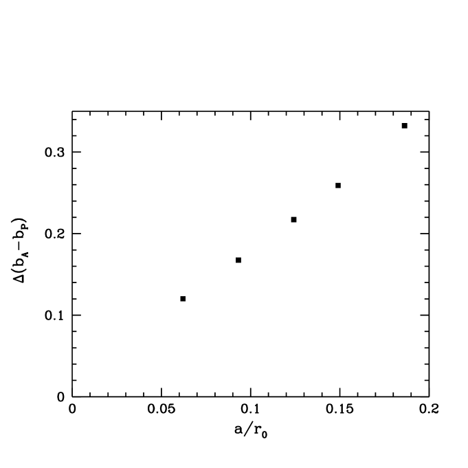
Figure 6: The difference $\Delta(b_{\rm A}-b_{\rm P})$ versus $a/r_{0}$.

4.6 Determination of $Z$

For the determination of the renormalization constant in the O($a$) improved theory we would like to keep the physics fixed up to errors of O($a^{2}$). Fortunately this is already the case, for the smallness of $b_{\rm A}-b_{\rm P}$ implies that the renormalized O($a$) improved quark masses are constant in units of $L$ with good numerical precision (cp. fig. 3).

Figure 7: Results for $Z$ as a function of $g_{0}^{2}$ from numerical simulations (filled squares) and 1-loop perturbation theory (dashed line). The solid line represents the fit function (4.45).

Figure 8: This plot shows the difference between the estimates of $Z$ obtained from two alternative renormalization conditions.

To evaluate the estimator $R_{Z}$ one needs the combination of improvement coefficients $b_{\rm A}-b_{\rm P}-b_{\rm m}$ [cp. eq. (2.30)]. We here simply insert the value obtained with the fit functions (4.38) and (4.42). At the largest lattice size of our simulations $g_{0}$ is outside the range of validity of (4.42). We use a linear fit to the last three data points for $b_{\rm m}$ to extrapolate our data to this point. The resulting systematic error can be estimated by calculating $Z$ with different values for $b_{\rm m}$. We find that it is smaller than $10^{-4}$ and will neglect it in the following. Our results for $Z$ are summarized in the fourth column of table 4 and shown in figure 7. In the range of couplings considered we find that our data is represented by the fit function

$$Z(g_{0}^{2})=(1+0.090514\ g_{0}^{2})\times{{1-0.9678\ g_{0}^{2}+0.04284\ g_{0}^{4}-0.04373\ g_{0}^{6}}\over{1-0.9678\ g_{0}^{2}}},$$ (4.45)

with a relative precision better than $0.04\%$. Again the perturbative result (2.34) has been incorporated into the fit.

It is important to check that another determination of $Z$ differs by O($a^{2}$). In fig. 8 we plot the difference between $R_{Z}$ determined with the improved and with the standard lattice derivatives versus $a^{2}/r_{0}^{2}$ and see the expected roughly linear dependence.

5 Summary and Conclusion

We have carried out a detailed non-perturbative determination of the improvement coefficients $b_{\rm m}$ and $b_{\rm A}-b_{\rm P}$ for the range of $\beta$ values used in present large scale simulations. In the case of $b_{\rm A}-b_{\rm P}$ we find that the typical O($a$) ambiguity at $\beta=6.0$ is not small. Rather than quoting a corresponding systematic error we advocated the use of improvement conditions at constant physics. This generalizes the strategy previously applied to renormalization constants [?]. As a result, we have obtained the improvement coefficients as smooth functions of the bare coupling [eqs. (4.38),(4.42)], and we checked that other choices of improvement condition lead to differences which vanish with a rate proportional to $a/r_{0}$. As a byproduct of our approach we also obtained the finite renormalization constant $Z=Z_{\rm m}Z_{\rm P}/Z_{\rm A}$, eq. (4.45). The same remarks as above apply to this case, except that the difference to other determinations vanishes with a rate proportional to $a^{2}/r_{0}^{2}$. In contrast to the improvement coefficients, our result for $Z$ differs from 1-loop perturbation theory in the bare coupling by no more than 3%.

Imposing physical improvement conditions and the error analysis are facilitated by the use of the Schrödinger functional technology and the use of simple direct estimators. It would be more difficult to ensure the constant physics condition if smearing techniques were necessary to enhance the signal, or if the improvement coefficients were obtained through a fitting procedure. Nevertheless, where they overlap, our new results are compatible with those of ref. [?] within the O($a$) and O($a^{2}$) ambiguities discussed in this paper. A drawback of the present method is that in the case of $b_{\rm m}$ we reached the limit of single precision arithmetic, because the estimator of this coefficient relies on the cancellation between bare quark masses which only happens up to rounding errors. As explained in detail, this problem becomes more pronounced as the lattice size increases and prevented us from using our largest lattice for an estimate of $b_{\rm m}$. We note that the strategy proposed here may be applied in other cases and may certainly be combined with the ideas of refs. [?,?] in order to determine the coefficients $b_{\rm A}$ and $b_{\rm P}$ separately.

We end with some comments concerning the coefficient $c_{\rm A}$ and the magnitude of the corrections associated with $b_{\rm A}-b_{\rm P}$ and $b_{\rm m}$. Since the original non-perturbative determination in ref. [?] the relatively large value of $c_{\rm A}$ at $\beta=6.0$ (as compared to one-loop perturbation theory) has been subject to doubts by other authors [?,?]. In these papers, an alternative determination of $c_{\rm A}$ was presented which yields a numerical value which is roughly half as big at $\beta=6.0$. One should note, however, that all the scaling tests that have been carried out for physical quantities [?,?] show the expected O($a$) improved continuum approach, albeit with sizable O($a^{2}$) artifacts in some cases. Our present work contains additional examples of scaling. In fact, the quantities shown in figures 6 and 8 have the advantage that they constitute pure lattice artifacts (rather than having an a priori unknown continuum limit). More precisely, $\Delta b_{\rm m}$ and $\Delta(b_{\rm A}-b_{\rm P})$ have to vanish in the limit $a/r_{0}=0$ only when the theory is order $a$ improved, i.e. when $c_{\rm sw}$ and $c_{\rm A}$ have the proper values. Similarly $\Delta Z={\rm O}(a^{2})$ is true only in this case. The convincing agreement with the expected behavior (cf. figs. 6 and 8) therefore constitutes new evidence that ${\rm O}(a)$ improvement has been correctly implemented.

We have emphasized above, that in taking the continuum limit of physical quantities the correct dependence of the improvement coefficients on $g_{0}$ is crucial. In addition, their overall magnitude determines whether they are relevant in practical applications. As we are considering coefficients multiplying quark masses, this depends in particular on whether one is interested in the physics of light quarks or heavy quarks. In the range of bare couplings considered, the bare strange quark mass in lattice units is smaller than $0.04$ [?]. Therefore, approximating the $b$-coefficients determined here by 1-loop perturbation theory (as has been done in [?]) does not introduce errors beyond the percent level for light quarks. On the other hand, for quark masses around the charm quark mass, non-perturbative values should be used if one is interested in precisions of a few percent. In addition, the difference $\Delta(b_{\rm A}-b_{\rm P})$ translates into an effect of about 10% for the situation of a D-meson [?] at $\beta=6.0$ and about half as much at $\beta=6.2$. Unless one takes the continuum limit, this is the magnitude of O$(a^{2}m_{\rm q})$ effects to be expected for D-mesons in the improved theory and one may suspect O$(a^{2}m_{\rm q}^{2})$ terms to be even larger.

This work is part of the ALPHA collaboration research programme. We would like to thank G. de Divitiis and M. Kurth for collaboration in the early stages of this work. Computer time on the Quadrics machines at DESY-Zeuthen and the University of Rome “Tor Vergata” is gratefully acknowledged. S. Sint acknowledges support by the European Commission under grant No. FMBICT972442. J. Rolf acknowledges a postdoc fellowship by Deutsche Forschungsgemeinschaft (Graduiertenkolleg GK271).

References

- [1] K. Jansen et al., Phys. Lett. B372 (1996) 275
- [2] R. Sommer, Nucl. Phys. Proc. Suppl. 42 (1995) 186
- [3] K. Symanzik, Some topics in quantum field theory, in: Mathematical problems in theoretical physics, eds. R. Schrader et al., Lecture Notes in Physics, Vol. 153 (Springer, New York, 1982)
- [4] K. Symanzik, Nucl. Phys. B226 (1983) 187 and 205
- [5] M. Lüscher and P. Weisz, Commun. Math. Phys. 97 (1985) 59, E: Commun. Math. Phys. 98 (1985) 433
- [6] B. Sheikholeslami and R. Wohlert, Nucl. Phys. B259 (1985) 572
- [7] M. Lüscher, S. Sint, R. Sommer and P. Weisz, Nucl. Phys. B478 (1996) 365
- [8] M. Lüscher, S. Sint, R. Sommer, P. Weisz and U. Wolff, Nucl. Phys. B491 (1997) 323
- [9] K. Jansen and R. Sommer, Nucl. Phys. B530 (1998) 185
- [10] M. Guagnelli and R. Sommer Nucl. Phys. B (Proc. Suppl.) 63 (1998) 886
- [11] T. Bhattacharya, S. Chandrasekharan, R. Gupta, W. Lee and S. Sharpe, Phys. Lett. B461 (1999) 79
- [12] T. Bhattacharya, R. Gupta, W. Lee and S. Sharpe, Nucl. Phys. B (Proc. Suppl.) 83 (2000) 851
- [13] T. Bhattacharya, R. Gupta, W. Lee and S. Sharpe, Nucl. Phys. B (Proc. Suppl.) 83 (2000) 902
- [14] G. De Divitiis and R. Petronzio, Phys. Lett. B419 (1998) 311
- [15] R. Gupta, talk given at Lattice 2000, Bangalore (India), to be published
- [16] M. Lüscher, S. Sint, R. Sommer and H. Wittig, Nucl. Phys. B491 (1997) 344
- [17] R. Wohlert, Improved continuum limit lattice action for quarks, DESY preprint 87-069 (1987), unpublished
- [18] M. Lüscher and P. Weisz, Nucl. Phys. B479 (1996) 429
- [19] S. Sint and R. Sommer, Nucl. Phys. B465 (1996) 71
- [20] S. Sint and P. Weisz, Nucl. Phys. B502 (1997) 251; Nucl. Phys. B (Proc. Suppl.) 63 (1998) 856
- [21] S. Capitani, M. Lüscher, R. Sommer and H. Wittig (ALPHA coll.), Nucl. Phys. B544 (1999) 669
- [22] J. Garden, J. Heitger, R. Sommer and H. Wittig (ALPHA and UKQCD colls.), Nucl. Phys. B571 (2000) 237
- [23] M. Lüscher, R. Narayanan, P. Weisz and U. Wolff, Nucl. Phys. B384 (1992) 168
- [24] S. Sint, Nucl. Phys. B421 (1994) 135
- [25] E. Gabrielli, G. Martinelli, C. Pittori, G. Heatlie and C.T. Sachrajda, Nucl. Phys. B362 (1991) 475
- [26] S. Sint, private notes (1996), unpublished
- [27] R. Sommer, Nucl. Phys. B411 (1994) 839
- [28] M. Guagnelli, R. Sommer and H. Wittig (ALPHA coll.), Nucl. Phys. B535 (1998) 389
- [29] S. Sint and P. Weisz (ALPHA coll.), Nucl. Phys. B545 (1999) 529
- [30] R. Frezzotti, M. Hasenbusch, J. Heitger, K. Jansen and U. Wolff, Comparative Benchmarks of full QCD Algorithms, in preparation
- [31] M. Guagnelli and R. Sommer, private notes (1998), unpublished
- [32] J. Heitger (ALPHA coll.), Nucl. Phys. B557 (1999) 309
- [33] M. Guagnelli, J. Heitger, R. Sommer and H. Wittig (ALPHA coll.), Nucl. Phys. B560 (1999) 465
- [34] K.C. Bowler et al. (UKQCD coll.), hep-lat/0007020