Vortices and monopole distributions in $Z(2)\times SO(3)$ lattice gauge theory

Abstract

We examine the occurance of $Z(2)$ and $SO(3)$ vorticies and monopole distributions in the neighborhood of Wilson loops. We use the Tomboulis formulation, equivalent to the Wilson action, in which the links are invariant under $Z(2)$ transformations and new plaquette variables carry the $Z(2)$ degrees of freedom. This gives new gauge invariant observables to help gain insight into the area law and structure of the flux tube.

$SU(N)$ lattice gauge theory with a Wilson action can be reformulated in terms of $Z(N)$ and $SU(N)/Z(N)$ variables as derived by Tomboulis[1] and Kovacs and Tomboulis[2]. We report results of simulations in these variables using an algorithm described elsewhere[3].

For the case considered here the $SU(2)$ group summation becomes an $SU(2)/Z(2)=SO(3)$ integration over the links (bonds), $U(b)$, and a discrete sum over the independent Z(2) variables, $\{\sigma(p)\}$, living on plaquettes. There are also dependent plaquette $Z(2)$ variables, $\{\eta(p)\}$, functions of $\{U(b)\}$, defined by $Tr[U(\partial p)]=\eta(p)|Tr[U(\partial p)]|$.

$$Z=\int\left[dU(b)\right]\sum_{\sigma(p)}\prod_{c}\delta[\sigma(\partial c)\eta(\partial c)]\times$$

$$\exp\left(\beta\sum_{p}\frac{1}{2}|\hbox{\small tr}[U(\partial p)]|\sigma(p)\right).$$

The expression for a Wilson loop, $W_{C}$, includes a tiling of any surface $S=\partial C$,

$$W_{C}=\sigma(S)\eta(S)\frac{1}{2}tr[U(\partial S)].$$ (1)

Note that $W_{1\times 1}=\sigma(p)\frac{1}{2}|tr[U(\partial p)]|$.

The excitations in this formulation include co-closed $2d$ vortex sheets which provide a mechanism to disorder the Wilson loop. They are more easily visualized in the dual representation where they consist of closed tiled sheets of either negative $\sigma(p)$ or negative $\eta(p)$ variables living on dual plaquettes. Each species form ‘open vortex patches’, (which we call ‘patches’) on the surface bounded by its corresponding species of a closed monopole loop living on dual links. We denote the boundary of patches of $\sigma(p)=-1$ as a $Z(2)$ monopole current and similarly $SO(3)$ monopole current surrounding the $\eta(p)=-1$ patches.

Constraints in the partition function enforce this vortex structure by requiring that any $Z(2)$ monopole loop be coincident with an $SO(3)$ monopole loop thus closing the surface. (This is the dual description of the cubic constraints in $Z$.) This gives a ‘hybrid’ vortex. The degenerate cases consist of a pure $\sigma(p)$ or a pure $\eta(p)$ vortex.

We are interested in sign fluctuations which disorder the Wilson loop. In order to clarify the simulation results below, consider first a simplified configuration $\{U(b),\sigma(p)\}$ for which a particular Wilson loop, has the value $=-1$ and further all links on $C$ $=I$, and only one of the tiling factors in Eqn.(1) is $-1$. And we also take a particular spanning surface $S$ e.g. the minimal surface.

1. Suppose that all $\sigma(p)=\eta(p)=+1$ on $S$ except for one negative $\sigma(p)$.

2. Then we can conclude that either (i) a $\sigma(p)$ vortex links the loop or (ii) a hybrid vortex links the loop with a $\sigma(p)=-1$ patch occurring on this particular surface.

3. Consider all distortions of $S$. If the negative sign is found to switch from a $\sigma(p)$ to the $\eta(p)$, then this is case (ii), a hybrid vortex links the loop.

4. If the signs of $\eta(p)$ and $\sigma(p)$ do not depend on $S$ then we are seeing case (i), a $\sigma(p)$ vortex linking the loop.

5. Suppose instead all $\sigma(p)=\eta(p)=+1$ on $S$ except for one negative $\eta(p)$ (instead of one negative $\sigma(p)$), and that this persists for all distortions of $S$ then we are seeing case(iii), an $\eta(p)$ vortex linking the loop.

The $\sigma(p)$ vortices (or patches) are known as ‘thin’ vortices (or patches). Thin vortices are suppressed at large $\beta$ because they cost action proportional to the vortex area and can at most disorder the perimeter of a Wilson loop. However thin patches do not suffer this limitation and indeed do contribute to Wilson loops in the data reported here.

The $\eta(p)$ vortices (or patches) are indicators of true ‘thick’ vortices (or patches) due to vorticity in $\{U(b)\}$. This is complicated by the fact $\eta(p)$ patches can be distorted with no cost of action because the links are SO(3) configurations, invariant under flipping the signs of links. An $\eta(p)$ vortex or patch can be moved to change the linkage number in $C$. However in the above example this would flip the sign of a link in $C$. The combination $\eta(S)\frac{1}{2}tr[U(\partial S)]$ is invariant under these sign flips and we use this to detect the presence of a thick vortex patch piercing $S$.

Following the studies in related work by Greensite et. al. [4] on projection vortices we use linkage numbers to tag Wilson loops and segregate then before computing averages. We count patches, mod 2, piercing the minimal surface using the operators[1, 2]

$${\cal N}_{\hbox{\small thin patch}} = \sigma_{S},$$ (2)

$${\cal N}_{\hbox{\small thick patch}} = \eta_{S}\hbox{\small sgn}\{tr[U(\partial S)]\}.$$ (3)

(Since we do not measure on every $S$, we can not discriminate between hybrid and thin or hybrid and thick linkage numbers.)

Fig. 1 gives the fraction $X_{e}$ of Wilson loops tagged to have 0 mod 2 vortices as a function of Wilson loop area on a $12^{4}$ lattice at $\beta=2.5$ ($X_{e}+X_{o}=1$, where $X_{o}$ is the 1 mod 2 fraction). The dashed curve corresponds to ${\cal N}_{\hbox{\small thin patch}}$, the dotted curve to ${\cal N}_{\hbox{\small thick patch}}$ and the solid curve to the product, i.e. tagged by the sign of the Wilson loop itself.

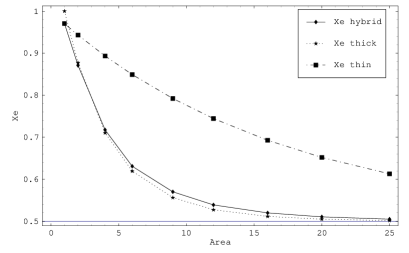
Figure 1: $X_{e}$ vs. area

For large areas, all curves approach $0.5$ giving nearly equal probabilites of an even or odd vortex number. Qualitatively, the rate of approach is a measure of the number of vortices per unit area piercing the minimal surface $S$. Clearly the thin patches are the least dense in this sense.

An interesting feature is that two curves cross. If the occurance of thin and thick patches were statistically independent, then counting either one (solid line), would be closer to the asymptotic value of $X_{e}$ and hence must lie below the two individual cases. A non-zero probablity of pairing of thin and thick patches might account for this crossing.

Figure 2: $W,W_{e},W_{o}$ vs. area for $\beta=2.3$

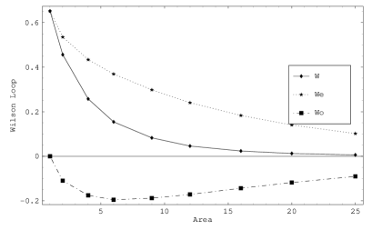
Figure 3: $W,W_{e},W_{o}$ vs. area for $\beta=2.5$

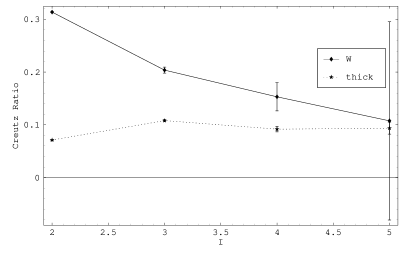
Figure 4: creutz raios $\chi(I,I)$ (solid line) and $\chi_{e}(I,I)$ (dotted line) for $\beta=$ $2.3$ (upper) and $2.5$ lower.

Figs. 2 and 3 give $W,W_{e}$ and $W_{o}$ as a function of area for $\beta=2.3$ and $\beta=2.5$. The dotted curve, $W_{e}$ corresponds to ${\cal N}_{\hbox{\small thick patch}}=0$, the dashed curve, $W_{o}$ to ${\cal N}_{\hbox{\small thick patch}}=1$ and the solid curve, $W$ to the Wilson loop itself. The values of $W_{e}$ and $W_{o}$ at area $=1$ follows from Eqns.(1) and (3). The exponential fall off follows from the fact that thin patches are still active in disordering this loop.

The dotted lines in Fig.4 are Creutz ratios, $\chi_{e}(I,I)=-\ln\frac{W_{e}(I,I)W_{e}(I-1,I-1)}{W_{e}(I,I-1)^{2}}$. Hence $W_{e}$ is showing an area law due to thin patches alone disordering the loop. We also plot $\chi(I,I)$ corresponding to $W$ for comparison. Poor statistics precludes a scaling analysis. Nevertheless the disordering due to thin patches compared to the full disordering is very similar for this range of $\beta$.

Finally we report the monopole density, $j_{m}$

$$\beta=2.3: 0.2156(4)$$

$$\beta=2.5: 0.142(1)$$

We also measured this within the flux tube

$$\langle j_{m}\rangle_{W}=\langle Wj_{m}\rangle/\langle W\rangle-\langle j_{m}\rangle.$$

We found that the monopole density was suppressed there. Details will appear elsewhere.

We thank E.T.Tomboulis for helpful discussions.

References

- [1] E. Tomboulis, Phys. Rev. D 32, 2371 (1981).
- [2] T. G. Kovacs and E. Tomboulis Phys. Rev. D 57, 4054 (1998).
- [3] A. Alexandru and R. Haymaker, hep-lat/0002031, to be published in Phys. Rev. 031017PRD.
- [4] M. Faber, J. Greensite and S. Olejnik, JHEP 9901:008,1999; JHEP 9912:012,1999; hep-lat/9911006; hep-lat/9912002.