SIMULATIONS IN $SO(3)\times Z(2)$ LATTICE GAUGE THEORY

Abstract

We explore simulations on periodic lattices in the Tomboulis $SO(3)\times Z(2)$ formulation. We measure gauge invariant vortex counters for “thin”, “thick” and “hybrid” vortex sheets in order to tag Wilson loops by the occurance of gauge invariant vortices linking them. We also measure projection vortex counters defined in the maximal center gauge for comparison.

1 Introduction

Lattice QCD continues to maintain an important role in the search for the physics of color confinement. The lattice regulator maintains gauge invariance at all costs. Dynamical variables are group elements rather than elements of a Lie algebra. As a consequence many of the topological features that are prominent candidates for elucidating the physics of confinement have natural lattice definitions. These include U(1), Z(N), SU(N)/Z(N) monopole loops, Dirac sheets, Z(N) and SU(N) vortex sheets etc. These objects are often abundant in U(1) and SU(N) lattice gauge theories. They become singular only as one approaches the continuum limit.

Yaffe [1], Tomboulis [2] and Kovacs and Tomboulis [3] have developed a formulation of SU(N) gauge theory that is manifestly SU(N)/Z(N) invariant. In this formulation, center elements, Z(N), multiplying each link leave the action and measure invariant. New Z(N) variables, defined on plaquettes, $\sigma(p)$, carry the Z(N) degrees of freedom. This formalism, equivalent to the standard SU(N) form, allows an elegant topological classification of the SU(N)/Z(N) and Z(N) vortex configurations occuring on the lattice. See also Refs. 4 - 7.

This talk is a report on our paper [8], in which we address the issues of simulations in the Tomboulis variables on a periodic lattice. Many results have followed from this formulation without doing simulations [9]. As a first calculation, we tag Wilson loop measurements by the occurance of vortices linking the loop using a number of different vortex counters. We restrict our attention to SU(2).

We also measure the P (projection) vortex counter in the original SU(2) formulation following Refs. 10 - 18 for comparison. Projection vortices arise in a Z(2) gauge theory derived from the original SU(2) theory by going to the maximal center gauge and then replacing links by $\hbox{\small sgn}(\hbox{\small tr}(U_{x,\mu}))$. The projected theory has “thin” Z(2) vortices defined on one lattice spacing. They have been found to be correlated with center vortices and therefore a measurement of P vortices is a predictor of them.

2 $Z_{Z(2)\times SU(2)/Z(2)}$ on a torus

The Wilson form of the partition function,

$$Z=\int\left[dU(b)\right]\exp\left(\beta\sum_{p}\frac{1}{2}\hbox{\small tr}[U(\partial p)]\right),$$ (1)

can be cast into a form in which the variables transform under $Z(2)$ and $SU(2)/Z(2)=SO(3)$ separately [2, 3, 8].

$$Z = \int\left[dU(b)\right]\sum_{\sigma(p)}C[\sigma(p)\eta(p)]\exp\left(\beta\sum_{p}\frac{1}{2}|\hbox{\small tr}[U(\partial p)]|\sigma(p)\right),$$ (2)

where

$$C[\sigma(p)\eta(p)]=\sum_{\tau(p)}\prod_{p}\chi_{\tau(p)}\left(\sigma(p)\eta(p)\right)\prod_{b}\delta\left(\tau(\widehat{\partial}b\right).$$ (3)

The derivation makes use of the invariance of the Haar measure under $Z(2)$ transformations $U(b)\rightarrow U(b)\gamma(b)$ of the links. Summing over $\gamma(b)$, the link matrices become $SU(2)$ representatives of the invariance group $SU(2)/Z(2)=SO(3)$. The $Z(2)$ dependence is transferred to new variables defined on plaquettes $\sigma(p)$. The variable $\eta(p)$ is the sign of the plaquette $\hbox{\small tr}[U(\partial p)]=|\hbox{\small tr}[U(\partial p)]|\times\eta(p)$.

$C[\sigma(p)\eta(p)]$ is a constraint, equal to either a positive constant or zero. The $Z(2)$ character, $\chi_{\alpha}(\beta)=\pm 1$, where $\alpha=\pm 1$ labels the representation and $\beta=\pm 1$ is the argument. $\chi_{+}(+)=\chi_{+}(-)=\chi_{-}(+)=-\chi_{-}(-)=+1$. The delta function constrains the $\tau$ summation to contribute only if an even number of negative $\tau$ plaquettes are in the coboundary of each link.

For free boundary conditions [2]

$$C[\alpha(p)]=\prod_{c}\delta\left(\alpha(\partial c)\right)\times\hbox{\small constant}$$

This requires that there be an even number of $\alpha(p)=\sigma(p)\times\eta(p)$ plaquettes on the faces of all elementary cubes.

3 Zero weight configurations on the torus

This constraint $C[\alpha(p)]$ is further restrictive for periodic boundary conditions. It gives zero for a vortex configuration of negative plaquettes on a coclosed surface wrapping around the torus. This means that one can not excite a configuration corresponding to the topologically stable anti-periodic boundary conditions and vice versa.

To see this we use a result from Ref. [8] Note that the $\{\tau\}$ configurations form a group with multiplication rule $(\tau_{1}\tau_{2})(p)=\tau_{1}(p)\tau_{2}(p)$. Using the invariance of the group sum over $\tau$ we can write

$$C[\alpha(p)] = \sum_{\tau(p)}\prod_{p}\chi_{\tau(p)}\left(\alpha(p)\right)\prod_{b}\delta\left(\tau(\widehat{\partial}b)\right),$$

$$= \sum_{\tau(p)}\prod_{p}\chi_{\tau_{0}(p)\tau(p)}\left(\alpha(p)\right)\prod_{b}\delta\left(\tau(\widehat{\partial}b)\right),$$

$$= \langle\tau_{0},\alpha\rangle\times C[\alpha(p)],$$

where $\langle\tau,\alpha\rangle\equiv\left\{\prod_{p}\chi_{\tau(p)}\left(\alpha(p)\right)\right\}$. If we can find a group element $\tau_{0}$ for which $\langle\tau_{0},\alpha\rangle\neq 1$ then $C[\alpha]=0$.

Take the example of a coclosed stack of $\alpha=-1$ (1,2) plaquettes at locations $(0,0,\xi,\eta)$ and a closed tiled surface of $\tau=-1$ (1,2) plaquettes at locations $(\mu,\nu,0,0)$. They have one plaquette in common, giving one factor of $-1$ in $\langle\tau_{0},\alpha\rangle$, and hence $C[\alpha]=0$.

As a second example let us consider how $C[\alpha]$ gives the cube constraint. Let us suppose that a particular cube violates this constraint with an odd number of faces with $\alpha=-1$. Then take a configuration $\tau_{0}$ which takes values $-1$ on all 6 faces of this particular cube. This is a closed surface and therefore satisfies the constraints imposed on $\tau$. Again $\prod_{p}\chi_{\tau_{0}(p)}\left(\alpha(p)\right)=-1$ and therefore $C[\alpha]=0$.

4 $\sigma(p)$ configuration space

We are interested in simulating in the variables $\{U(b),\sigma(p)\}$. Allowed configurations $\alpha(p)$ are defined indirectly by the constraint, function $C[\alpha]$. The corresponding simulation would be cumbersome to implement.

We proposed [8] a constructive definition of allowable $\alpha(p)$ configurations by building them up from “star transformations”, i.e. correlated sign flips of the $\sigma$ plaquettes occurring in the co-boundary of each link. We showed [8] that the constrained updates of six plaquettes reaches all allowed $\{\sigma\}$ configurations, and in fact is identical to the above definition. In this section we summarize this result.

Before discussing the $\sigma$ configurations let us first describe the link updates. This is a straightforward generalization of the link updates for $SU(2)$. The proposed change in a link might change the sign of the $\eta$ plaquettes in the co-boundary of the link. If one of these changes sign, we need to flip the sign of the corresponding $\sigma$ plaquette so that the $\alpha$ configuration is unchanged. Then the Monte Carlo step is essentially the same as for the SU(2) update.

Next consider the above mentioned star transformations. Our proposed update is to flip the sign of the six $\sigma$ plaquettes forming the co-boundary of the links.

It is easy to see that both these update steps will preserve the local constraints, i.e. the cube constraints.

Next examine the global constraints. Consider the operator constructed out of $\mu,\nu$ plaquettes [3]

$${\cal N}_{\mu,\nu}=\prod_{p\in S_{\mu,\nu}}\eta(p)\sigma(p)\equiv\eta(S_{\mu,\nu})\sigma(S_{\mu,\nu})=\pm 1,$$

where $S_{\mu,\nu}$ is a whole tiled $\mu,\nu$ plane. ${\cal N}_{\mu,\nu}=\pm$ for an even/odd number of vortices of stacked $\mu,\nu$ plaquettes wrapping around the orthogonal $\xi,\eta$ directions of the torus.

We start with ${\cal N}_{\mu,\nu}=+1$ in all 6 planes. It is easy to see that our update algorithm preserves ${\cal N}_{\mu,\nu}$.

Let us define the relevant sets of configurations more carefully.

$$C[\alpha] \equiv \sum_{\tau(p)}\prod_{p}\chi_{\tau(p)}\left(\alpha(p)\right)\prod_{b}\delta\left(\tau(\widehat{\partial}b)\right),$$ (4)

$$= \sum_{\tau\in{\cal C}}\prod_{p}\chi_{\tau(p)}\left(\alpha(p)\right),$$

$$\equiv \sum_{\tau\in{\cal C}}\langle\tau,\alpha\rangle\;\;\;=\;\;\;\sum_{\tau\in{\cal C}}\langle\alpha,\tau\rangle.$$

The bracket, $\langle\alpha,\tau\rangle=\pm 1$, is negative if and only if there are an odd number of plaquettes for which both $\alpha(p)=-1$ and $\tau(p)=-1$.

The second line is an alternative way to specify the sum, where:

$${\cal C}=\{\tau\in{\cal A}|\prod_{b}\delta\left(\tau(\widehat{\partial}b)\right)=1\}.$$

${\cal C}$ is a subgroup of the group ${\cal A}$ of all configurations, $|{\cal A}|=2^{6N}$ in number, where $N$ is the number of lattice sites. ${\cal C}$ is the group of all configurations $\{\tau\}$ with an even number of $\tau=-1$ plaquettes occurring in the co-boundary of every link, i.e. forming a closed tiled surface of negative plaquettes.

There is a second group of interest,

$$\overline{\cal C}=\{\alpha\in{\cal A}|\langle\alpha,\tau\rangle=1\;\;\;\;\forall\tau\in{\cal C}\}.$$

${\overline{\cal C}}$ is the group of all configurations $\{\alpha\}$ for which $C(\alpha)$ is different from zero.

Therefore ${\overline{\cal C}}$ is the group of $\alpha$ configurations which have non zero weight in the partition function, Eqn.(2). Further, ${\cal C}$ is the group of $\tau$ configurations that form closed tiled surfaces as required by the explicit constraints in Eqn.(4).

The group ${\cal C}$ has only an implicit definition here. The group ${\overline{\cal C}}$ has an implicit definition in terms of this ${\cal C}$. Therefore its definition is even more indirect. Even without an explicit definition, we have been able to specify precisely those configurations $\{\alpha\}$ that contribute non-zero weight to the partition function.

There is a third group of interest,

$${\cal D}=\{\alpha\in{\cal A}|\alpha=\prod\alpha_{\hat{\partial}b_{i}}\}.$$

where $\alpha_{\hat{\partial}b_{i}}$ refers to an individual star transformation on the $i$’th link $b_{i}$, and the product indicates all possible products of them. ${{\cal D}}$ is the group of all configurations $\{\alpha\}$ which can be built out of products of “star transformations” starting from the identity configuration.

This is the constructive definition that is straightforward to implement in a simulation. We show in Ref. [8] that the group $\cal D$ is identical to the group ${\overline{\cal C}}$. In this way we have shown that by our proposed algorithm is ergodic.

5 Simulation of vortex counters

Vortices have long been considered as prime candidates for the essential dynamical variable to describe confinement. A simulation offers a tool that allows one to correlate the occurance of vortices with values of other dynamical variables. Hence as a first application we use this formalism to measure various vortex counters for Wilson loops.

In the $SO(3)\times Z(2)$ formulation the Wilson loop is given by

$$W[C]=\langle\frac{1}{2}\hbox{\small tr}[C]\eta_{S}\sigma_{S}\rangle_{C=\partial S},$$

where $\eta_{S}$ and $\sigma_{S}$ are products of $\eta$ and $\sigma$ over any spanning surface [1, 2, 3].

Kovacs and Tomboulis [3] define three vortex counters for thick vortex sheets, thin vortex sheets, and hybrid (patches of each on the sheet).

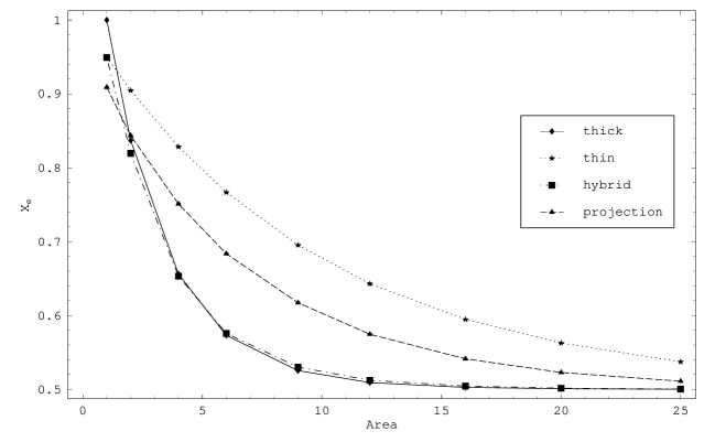
Figure 1: Fraction of Wilson loops with an even number of vortices piercing the minimal surface, $x_{e}$. ($x_{o}=1-x_{e}$)

Figure 2: Wilson loop, W, and tagged Wilson loop with even or odd number of “thick” vortices piercing the minimal surface.

Thin:

$${\cal N}_{\hbox{\small thin}}\equiv\sigma_{S}.$$

If this value, $=\pm 1$, is independent of the spanning surface, then this counts thin vortices.

Thick:

$${\cal N}_{\hbox{\small thick}}\equiv\eta_{S}\;\hbox{\small{sgn}[tr}W(C)].$$

This object is counting something more elusive since unlike the above case, the vortex structure is spread over many lattice spacings. Nevertheless it is always possible to find a representative of SO(3) such that the $\eta$ vortex defines the topological linkage [3]. The $\eta$ vortices can be deformed by a $Z(2)$ transformation of links giving different representatives of SO(3) without cost of action. One can move a linked $\eta$ vortex sheet so that it no longer links the Wilson loop and further even transform it away. However in this case the negative contribution will be transferred to one of the perimeter links of the Wilson loop, and it will not affect the value of ${\cal N}_{\hbox{\small thick}}$. Again if this is independent of the spanning surface, then this counts “thick” vortices.

Hybrid:

$${\cal N}_{\hbox{\small hybrid}}={\cal N}_{\hbox{\small thin}}\times{\cal N}_{\hbox{\small thick}}=\sigma_{S}\eta_{S}\;\hbox{\small{sgn}[tr}W(C)].$$

As one considers all spanning surfaces, the sign of ${\cal N}_{\hbox{\small thin}}$ might change. However if the sign of ${\cal N}_{\hbox{\small thick}}$ always compensates then this counts hybrid vortices.

6 Numerical Results

Figure 3: Wilson loop, W, and tagged Wilson loop with even or odd number of projection vortices piercing the minimal surface.

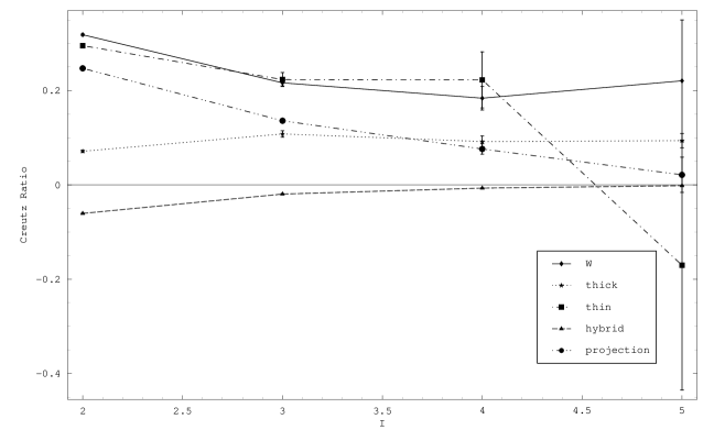
Figure 4: Creutz Ratio: $\chi(I,I)=-\ln\frac{W(I,I)W(I-1,I-1)}{W(I,I-1)^{2}}$, similarly for tagged Wilson loops $W_{e}$.

Simulations were done on a $12^{4}$ lattice for $\beta=2.30$. Measurements were binned to 10 bins and jackknife errors calculated. [thin]: 200 ; [thick]: 400 ; [hybrid]: 200 ; [projection]: 1000 measurements. We monitor the coincidence of Z(2) and SO(3) monopoles which can slip due to round off error.

Kovacs and Tomboulis’ definitions require measurements on all spanning surfaces. We measure here only the minimum spanning surface. Then, for example, ${\cal N}_{\hbox{\small thin}}=-1$ does not distinguish thin from hybrid, and similarly ${\cal N}_{\hbox{\small thick}}=-1$ does not distinguish thick from hybrid.

Fig. 1 shows the fraction of Wilson loops which have an even number of vortices, $x_{e}$, as a function of the area. All the counters approach $50\%$ from above with similar behavior ($x_{o}=1-x_{e}$). They are each counting different things and are not expected to be equal.

${\cal N}_{\hbox{\small hybrid}}$ is a good reference curve since it measures the sign of the Wilson loop itself. The area law arises from a near cancelation of fluctuating values due to approximately equal occurance and absence of thin, thick or hybrid vortices.

The “thick” curve lies on top of the “hybrid” one. Hence the added factor of $\sigma_{S}$ in the hybrid counter has little effect here. We expect $\sigma$ vortices to be heavily suppressed for increasing $\beta$ since they cost action proportional to the vortex area. However at $\beta=2.30$ the density of Z(2) (or SO(3)) monopoles $=0.2155(2)$ (Random plaquette signs would give a density of $~{}0.5$). Hence in spite of the near coincidence of these two curves, $\sigma$ vortices and $\sigma$ patches of hybrid vortices are important at this value of $\beta$. There is further evidence below. The ${\cal N}_{\hbox{\small projection}}$ case gives the same result as reported in Ref [10].

Fig.2 [Thick segment piercing the minimal surface] By definition $W_{e}$ has an even number of thick segments piercing the minimal surface. Yet it still has an exponential fall off with area. See Fig. 4 which gives the Creutz ratio showing that $W_{e}$ has about half the string tension of the $W$. The thin segments are still present and they account for the disordering.

Fig. 3 [Projection vortices piercing the minimal surface] For loops of area 9 and higher, the sign of the vortex counter correlates with $W_{o}$. These data agree with Ref. [10]. Comparing this with Fig. 2 [thick] the latter data are about a factor of 10 larger, indicating a large discrepancy in these two methods of tagging center vortices.

Fig. 4 [Creutz Ratio] $W$ and $W_{e}$ [thick] show a constant string tension for larger loops. We suspect that with better statistics, $W_{e}$ [thin] will also. $W_{e}$ [hybrid] shows the vanishing of the string tension if one removes the disordering mechanism completely. Larger loop areas are needed to decide if the Creutz Ratio of $W_{e}$ [projection] will also go to zero, or stabilize which would indicate that a disordering mechanism remains.

7 Summary

The Tomboulis formalism provides a precise way to separate the physical effects of thin and thick vortices. Simulations in these variables allows one to disentangle these effects as one approaches the continuum limit where thick vortices are expected to dominate.

References

References

- [1] L. G. Yaffe, Phys. Rev. D 21, 1574 (1980).
- [2] E. Tomboulis, Phys. Rev. D 32, 2371 (1981).
- [3] T. G. Kovacs and E. Tomboulis Phys. Rev. D 57, 4054 (1998)
- [4] G. Mack and V. B. Petkova, Annals of Physics 123, 442 (1979); 125, 117 (1980); Z. Phys. C 12, 177 (1982).
- [5] G. Halliday and A. Schwimmer, Phys. Lett. B 101, 327 (1981); B 102, 337 (1981).
- [6] T. Yonewa Nucl. Phys. B 203 [FS5], 130 (1982).
- [7] J. M. Cornwall, Phys. Rev. D 26, 1453 (1979)
- [8] A. Alexandru and R. W. Haymaker, hep-lat/0002031, to be published in Phys. Rev.
- [9] T. G. Kovacs and E. Tomboulis hep-lat/0002004, 9912051, 9908031, Phys. Lett. B 463 104 (1999); Nucl. Phys. B, Proc. Suppl 73566 (1999); Phys. Lett. 443 239, (1998); J. Math. Phys. 40, 4677 (1999).
- [10] L. Del Debbio, M. Faber, J. Greensite and S. Olejnik, Phys. Rev. D 55, 2298 (1997), hep-lat/9802003,
- [11] M. Faber, J. Greensite and S. Olejnik, JHEP 9901:008,1999; JHEP 9912:012,1999; hep-lat/9911006; hep-lat/9912002
- [12] J. Ambjorn, J. Giedt, J. Greensite, hep-lat/9907021, hep-lat/9908020
- [13] K. Langfeld and H. Reinhardt, Phys. Rev. D 55,7993 (1997)
- [14] K. Langfeld, H. Reinhardt and O. Tennert, Phys. Lett. B 419, 317 (1998);
- [15] M. Engelhardt, K. Langfeld, H. Reinhardt and O. Tennert, Phys. Lett. B 431, 141 (1998); 452, 301 (1999); Phys. Rev. D 61:054504,2000; hep-lat/9908026
- [16] P. de Forcrand and M. D’Elia, hep-lat/9907028; hep-lat/9909005.
- [17] A. Montero, hep-lat/9907024.
- [18] P. W. Stephenson, hep-lat/9909022.