CERN-TH/2000-259
NIC/DESY-00-001
Lattice hadron matrix elements with the Schrödinger functional: the case of the first moment of non-singlet quark density

We present the results of a non-perturbative determination of the pion matrix element of the twist-2 operator corresponding to the average momentum of non-singlet quark densities. The calculation is made within the Schrödinger functional scheme. We report the results of simulations done with the standard Wilson action and with the non-perturbatively improved clover action and we show that their ratio correctly extrapolates, in the continuum limit, to a value compatible with the residual correction factor expected from perturbation theory.

CERN-TH/2000-259

August 2000

The calculation of hadronic matrix elements of Wilson operators entering the light cone expansion of two electroweak currents, directly connected to the moments of parton density distributions, requires non-perturbative tools. Lattice estimates have been produced so far for only the first few such moments. The results for the second moment of non-singlet quark densities, corresponding to the average momentum, are typically higher than the experimental values. However, these results have been obtained at fixed lattice spacing only and using, as renormalization factor for the bare operator, the one obtained from a perturbative calculation. It is the aim of our alternative approach to remove these approximations.

The scope of the present paper is to provide values of the bare matrix element at different lattice spacing. After multiplication with the corresponding non-perturbative renormalization factor, these values can be used for an estimate of the continuum limit of the renormalized matrix element. In a series of papers, other essential ingredients needed for such an estimate were obtained. In particular, the Schrödinger functional (SF) renormalization scheme was discussed in [1], the non-perturbative step scaling function describing the scale evolution of the continuum renormalization factor in [2], the universality of the continuum limit of the step scaling function in [3] and the definition of a “renormalization group invariant” step scaling function in [4]. The pion matrix element has already been calculated for the Wilson action and with standard periodic boundary conditions [6]: here we want to show how the SF can be used to reliably calculate not only the renormalization factor but also the physical matrix element itself.

The use of the SF for extracting hadron correlation functions has been initiated with the calculation of pseudoscalar and vector masses and decay constants by the ALPHA collaboration [5]. The calculation with the SF of a two-quark matrix element has never been attempted before and, with respect to a traditional method, presents two advantages. The first is the possibility of constructing “smeared” and gauge-invariant states as particle sources at the boundary (for the pion in this case). The second advantage is that the choice of SF boundary conditions allows insertion of the operator at $T/2$, where $T$ is the total time extent of the lattice, to be compared with the maximum value $T/4$, reachable with ordinary periodic boundary conditions. If the operator of interest is inserted at a fixed physical distance, this amounts to needing a lattice for the SF that is a factor of 2 smaller in the time direction than the one using periodic boundary conditions.

In our previous work we have evaluated a non-perturbative renormalization factor of the following operator:

$${\cal O}_{12}(x)=\frac{1}{4}\bar{\psi}(x)\gamma_{\{1}\stackrel{{\scriptstyle\leftrightarrow}}{{D}}_{2\}}\frac{\tau^{3}}{2}\psi(x)\;,$$ (1)

where $\stackrel{{\scriptstyle\leftrightarrow}}{{D}}_{\mu}$ is the covariant derivative and the bracket around indices means symmetrization. The calculation of the matrix element of this operator requires a non-zero pion momentum. In practice, this leads to a very noisy signal for large time separation.

This has been observed also with periodic boundary conditions in ref. [6], but is even more crucial in our case, where we can reach a larger distance in time to project on the lightest state. We therefore decided to follow ref. [6] and compute numerically on the lattice the desired matrix element between pion states with a different lattice representation of the twist-2 operator than the one defined in eq. (1). This amounts to taking:

$${\cal O}_{00}(x)=\frac{1}{4}\bar{\psi}(x)\left[\gamma_{0}\stackrel{{\scriptstyle\leftrightarrow}}{{D}}_{0}-\frac{1}{3}\sum_{k=1}^{3}\gamma_{k}\stackrel{{\scriptstyle\leftrightarrow}}{{D}}_{k}\right]\frac{\tau^{3}}{2}\psi(x)\;.$$ (2)

The advantage of this operator is that it can be computed at vanishing external momentum and is hence expected to show a much better signal to noise behaviour than ${\cal O}_{12}$ and not to be contaminated too strongly by lattice artefacts. Indeed, as in [6], we find also within our SF calculation, the correlation function of ${\cal O}_{00}$ to be much less noisy than ${\cal O}_{12}$. In addition, we want to remark that we find with comparable statistics, the error of the matrixelement of the operator ${\cal O}_{00}$ to be considerably smaller when using SF than for periodic boundary conditions as used in [6].

Figure 1: The correlation function

The operator is inserted between two SF states defined at the two time boundaries, as depicted in fig. 1. We start by defining the boundary operators at the time boundaries $0$ and $T$:

$${\cal O}_{0}=\frac{a^{6}}{L^{3}}\sum_{\bf{y},\bf{z}}\bar{\zeta}({\bf{y}})\gamma_{5}\frac{\tau^{3}}{2}\zeta({\bf{z}}),\quad\quad\quad{\cal O}_{T}=\frac{a^{6}}{L^{3}}\sum_{\bf{y},\bf{z}}\bar{\zeta}^{\prime}({\bf{y}})\gamma_{5}\frac{\tau^{3}}{2}\zeta^{\prime}({\bf{z}})$$ (3)

and then the correlation function (of mass dimension equal to 1):

$$f_{\rm M}(x_{0})=a^{3}\sum_{\bf{x}}\langle{\cal O}_{0}{\cal O}_{00}(x){\cal O}_{T}\rangle\;.$$ (4)

We also consider, for purposes of normalization, the correlation function

$$f_{1}=-\langle{\cal O}_{0}{\cal O}_{T}\rangle\;.$$ (5)

Closely following the discussion in ref. [5], we easily see that for a time extent large enough, the matrix element is expected to be taken among the lightest particles coupled to the surface states, i.e. between pions, in our case. The general formulae, including the first excited state, are:

$$f_{1} \simeq \rho^{2}e^{-m_{\pi}T},$$

$$f_{\rm M}(x_{0}) \simeq \rho^{2}e^{-m_{\pi}T}\langle\pi|{\cal O}_{00}|\pi\rangle\left\{1+\rho^{\prime}e^{-\Delta x_{0}}+\rho^{\prime\prime}e^{-\Delta(T-x_{0})}\right\}\;.$$ (6)

The actual matrix element is obtained from $f_{\rm M}(x_{0})$ only after a suitable normalization by $f_{1}$, which takes out the effects (wave-function contribution) of the boundary quark fields. Assuming that there is a plateau region where $f_{M}(x_{0})/f_{1}=\mathrm{const}\equiv\langle\pi|{\cal O}_{00}|\pi\rangle$, and in which the first excited state gives essentially no contributions, we obtain the physical matrix element by a suitable normalization (see [6]):

$$\langle x\rangle\equiv\frac{2\kappa}{m_{\pi}}\langle\pi|{\cal O}_{00}|\pi\rangle\;,$$ (7)

with $\kappa$ the hopping parameter appearing in the fermion action. The value of the pion mass is obtained, following ref. [5], from the time dependence of the pseudoscalar ($f_{\rm P}$) and/or axial-vector ($f_{\rm A}$) correlation functions.

The set-up for our numerical simulation, performed in the quenched approximation, was to choose lattices of physical size $L^{3}\cdot T$, with $T$ taken to be $T\approx 3\;{\rm fm}$ in all calculations. We performed two sets of simulations, one using the Wilson action and a second, using the non-perturbatively improved clover action. The correlation function projects on a single pion state at a distance in time corresponding to about 1 fm. We then selected a time interval of 1 fm again to extract the matrix element. An example for the plateau behaviour of our correlation function and a fit to a plateau value with a distance of about 1 fm is shown in fig. 2.

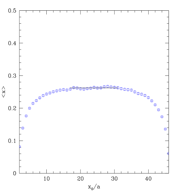
Figure 2: Example for the plateau behaviour of the correlation function $2\kappa/m_{\pi}\cdot f_{\rm M}(x_{0})/f_{1}$ to extract the matrix element, taken at $\beta=6.2$, $\kappa=0.1346$ on a $24^{3}\cdot 48$ lattice (clover action).

At each of our four values of $\beta=6/g_{0}^{2}$, the calculation of the matrix element is performed at three values of the quark masses, using a multiple mass solver. Table 1 contains all our results for the matrix element $\langle x\rangle$ at various values of the quark mass and of $\beta$, for both the Wilson and for the $\mathrm{O}(a)$-improved clover action. In fig. 3 we show one example for the chiral extrapolation of the matrix element.

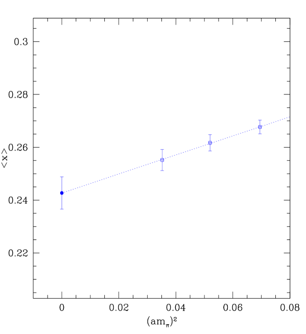
Figure 3: Example for the chiral extrapolation of the matrix element at $\beta=6.3$ using the clover action.

In table 2 we give the data for the matrix elements extrapolated to the chiral limit. They can now be used to test the continuum extrapolation, by building the ratio of the matrix elements calculated with the two different lattice actions we have used in our simulation. In fig. 5 we show these ratios as a function of the lattice spacing. The data are extrapolated to the continuum as a linear function of the lattice spacing. Given the limited range in the bare coupling where the data were collected, the extrapolation procedure only extrapolates lattice artefacts that vanish like a power of the lattice spacing. Logarithmically dependent corrections, i.e. terms proportional to the bare coupling, cannot be taken into account in this way. Then, the result of the continuum extrapolation of the ratio is not expected to be one, but the value of a correction factor evaluated at a bare coupling value of order $1$, corresponding to the region in $\beta$ where the extrapolation was made. The correction factor from a perturbative calculation at $g^{2}=1$ is $1.04$ [7]. Figure 5 shows that our data are very well compatible with such a value and gives us confidence in the uniqueness of the continuum limit.

We have also computed the renormalization factor $Z_{12}$ of the operator of eq. (1) at the smallest scale $\mu_{\mathrm{min}}$ we could reach in our previous work for the scale evolution, $\mu_{\mathrm{min}}^{-1}=1.436r_{0}$ with $r_{0}\approx 0.5\;\mathrm{fm}$. The values of $Z_{12}$ for our two lattice actions are shown in fig. 4 as a function of $\beta$. In the figure the physical scale $\mu_{\mathrm{min}}$ is kept fixed when varying $\beta$ by suitably choosing the lattice size. In order to obtain the renormalization constant at exactly the values of $\beta$ where the matrix element is computed, we performed an interpolation which is also given in the caption of fig. 4. We give the interpolated values of $Z_{12}$ in table 2.

If we would now use $Z_{12}$ to renormalize the operator ${\cal O}_{00}$, the extrapolation to the continuum limit of the renormalized pion matrix element of the operator ${\cal O}_{00}$ would acquire a similar correction factor, as in the case of the ratio of the bare matrix element as discussed above. This is why we do not proceed to extract directly from our matrix element its renormalized value in the continuum limit and we postpone to a forthcoming paper the non-perturbative evaluation of such a correction factor, which anyway is expected, from perturbation theory, to be of the order of a few per cent.

We have demonstrated in this paper that the SF calculation of hadron matrix elements is feasible and could be applied to other interesting cases, such as the operators arising from effective weak hamiltonians.

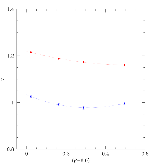
Figure 4: Non-perturbative evaluation of $Z_{12}$ at a fixed inverse scale $L=1.436\;r_{0}$. The upper curve is for clover-improved fermions, the lower one for Wilson fermions. The numbers quoted in table 2 follow from the following interpolations (shown as dotted lines), which we take as a definition of the two renormalization constants in this range of $\beta$ values:
$Z_{12}^{\rm C}=1.2196-0.2244(\beta-6)+0.2117(\beta-6)^{2},$
$Z_{12}^{\rm W}=1.0331-0.3570(\beta-6)+0.5714(\beta-6)^{2}$.

$\beta$	$\kappa$	Action	fit interval	$m_{\pi}$	$\langle x\rangle$
	$0.153$			$0.4183(14)$	$0.3096(17)$
$6.0$	$0.154$	W	$11-21$	$0.3594(15)$	$0.3005(22)$
	$0.155$			$0.2925(18)$	$0.2903(32)$
	$0.151605$			$0.3663(14)$	$0.3070(25)$
$6.1$	$0.152500$	W	$12-24$	$0.3104(16)$	$0.2967(33)$
	$0.153313$			$0.2528(19)$	$0.2862(47)$
	$0.150600$			$0.3139(9)$	$0.3035(19)$
$6.2$	$0.151300$	W	$17-31$	$0.2669(10)$	$0.2915(24)$
	$0.151963$			$0.2164(12)$	$0.2769(34)$
	$0.149259$			$0.2977(10)$	$0.3024(23)$
$6.3$	$0.149978$	W	$24-40$	$0.2490(12)$	$0.2874(33)$
	$0.150604$			$0.2007(15)$	$0.2703(56)$
	$0.1334$			$0.3988(11)$	$0.2701(15)$
$6.0$	$0.1338$	C	$11-21$	$0.3527(11)$	$0.2658(18)$
	$0.1342$			$0.3005(13)$	$0.2597(27)$
	$0.1340$			$0.3497(10)$	$0.2729(16)$
$6.1$	$0.1345$	C	$12-24$	$0.2919(12)$	$0.2671(21)$
	$0.1350$			$0.2223(14)$	$0.2612(40)$
	$0.1346$			$0.2796(7)$	$0.2624(16)$
$6.2$	$0.1349$	C	$17-31$	$0.2428(8)$	$0.2569(20)$
	$0.1352$			$0.2009(9)$	$0.2519(27)$
	$0.1346$			$0.2637(10)$	$0.2677(26)$
$6.3$	$0.1349$	C	$24-40$	$0.2281(11)$	$0.2617(31)$
	$0.1352$			$0.1876(13)$	$0.2552(40)$

Table 1: Our results for the two actions, Wilson (W) and non-perturbatively improved (C), that we have used. We also give the fit interval in $x_{0}/a$ corresponding to a distance of 1 fm.

$\beta$	$a$ (fm)	$T/a$	$L/a$	$Z_{12}$	$\langle x\rangle$	$N$
$6.0$	$0.093$	$32$	$16$	$1.033$	$0.2727(46)$	$600$
$6.1$	$0.079$	$36$	$16$	$1.004$	$0.2683(67)$	$573$
$6.2$	$0.068$	$48$	$24$	$0.985$	$0.2549(49)$	$416$
$6.3$	$0.059$	$64$	$24$	$0.977$	$0.2474(76)$	$391$
$6.0$	$0.093$	$32$	$16$	$1.2196$	$0.2471(44)$	$600$
$6.1$	$0.079$	$36$	$16$	$1.1993$	$0.2535(48)$	$800$
$6.2$	$0.068$	$48$	$24$	$1.1832$	$0.2405(41)$	$500$
$6.3$	$0.059$	$64$	$24$	$1.1713$	$0.2427(61)$	$319$

Table 2: Our results for the matrix element in the chiral limit at various values of the lattice spacing. We also give the renormalization factor $Z_{12}$ as obtained from interpolating the simulation data shown in fig. 4. The upper set of data belong to simulations with the Wilson action, the lower set to simulations with the clover action. In the last column we give the number $N$ of configurations as used for evaluating $\langle x\rangle$.

Figure 5: The continuum extrapolation of the ratio of the bare lattice matrix elements computed with the clover–improved and Wilson fermion action.

ACKNOWLEDGEMENTS

We have considerably profited from the experience accumulated by the ALPHA collaboration with the Schrödinger functional with fermions. We thank F. Palombi and A. Shindler for useful discussions.

References

-
[1]
A. Bucarelli, F. Palombi, R. Petronzio and A. Shindler,
Nucl. Phys. B552 (1999) 379
-
[2]
M. Guagnelli, K. Jansen and R. Petronzio,
Nucl. Phys. B542 (1999) 395
-
[3]
M. Guagnelli, K. Jansen and R. Petronzio,
Phys. Lett. B457 (1999) 153
-
[4]
M. Guagnelli, K. Jansen and R. Petronzio,
Phys. Lett. B459 (1999) 594
- [5] M. Guagnelli, J. Heitger, R. Sommer and H. Wittig, Nucl. Phys. B560 (1999) 465
- [6] C. Best et al., Phys. Rev. D56 (1997) 2743
- [7] S. Capitani et al., Nucl. Phys. B (Proc. Suppl.) 63 (1998) 874